Source Apportionment of Fine Particles in Tennessee Using a Source

TECHNICAL PAPER

ISSN:1047-3289 J. Air & Waste Manage. Assoc. 57:407– 419 DOI:10.3155/1047-3289.57.4.407 Copyright 2007 Air & Waste Management Association

Source Apportionment of Fine Particles in Tennessee Using a Source-Oriented Model Prakash Doraiswamy, Wayne T. Davis, Terry L. Miller, and Joshua S. Fu Department of Civil and Environmental Engineering, University of Tennessee, Knoxville, TN

ABSTRACT Source apportionment of fine particles (PM2.5, particulate matter ⬍ 2 ␮m in aerodynamic diameter) is important to identify the source categories that are responsible for the concentrations observed at a particular receptor. Although receptor models have been used to do source apportionment, they do not fully take into account the chemical reactions (including photochemical reactions) involved in the formation of secondary fine particles. Secondary fine particles are formed from photochemical and other reactions involving precursor gases, such as sulfur dioxide, oxides of nitrogen, ammonia, and volatile organic compounds. This paper presents the results of modeling work aimed at developing a source apportionment of primary and secondary PM2.5. On-road mobile source and point source inventories for the state of Tennessee were estimated and compiled. The national emissions inventory for the year 1999 was used for the other states. U.S. Environmental Protection Agency Models3/ Community Multi-Scale Air Quality modeling system was used for the photochemical/secondary particulate matter modeling. The modeling domain consisted of a nested 36 –12– 4-km domain. The 4-km domain covered the entire state of Tennessee. The episode chosen for the modeling runs was August 29 to September 9, 1999. This paper presents the approach used and the results from the modeling and attempts to quantify the contribution of major source categories, such as the on-road mobile sources (including the fugitive dust component) and coal-fired power plants, to observed PM2.5 concentrations in Tennessee. The results of this work will be helpful in policy issues targeted at designing control strategies to meet the PM2.5 National Ambient Air Quality Standards in Tennessee.

IMPLICATIONS A major fraction of the fine particle composition is believed to be secondary in nature formed through chemical reactions of precursor gases and not emitted directly. To better manage air quality, it is important to know the sources or source categories that contribute to ambient PM2.5 concentrations. Although receptor models have been used to do source apportionment, they do not fully take into account the chemical reactions involved in the formation of secondary fine particles. This paper uses a source-oriented photochemical model in identifying the major source categories of primary and secondary PM2.5 in Tennessee.

Volume 57 April 2007

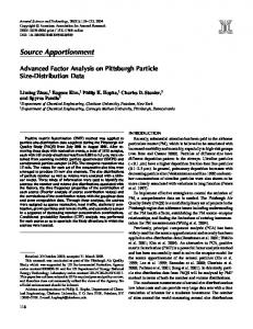
INTRODUCTION Fine particles (particulate matter [PM] ⬍2.5 ␮m in aerodynamic diameter [PM2.5]) are of concern because of their linked effects on health and on aesthetic issues, such as visibility. Some studies have linked PM2.5 concentrations to increased mortality rates.1 Fine particles also tend to scatter light and play a major role in light attenuation. Sulfates and organics in fine particles, in addition to other components, are believed to contribute significantly to light extinction.2,3 In the eastern part of the United States, it has been observed that sulfates account for ⬃56% of PM2.5 composition followed by organic carbon accounting for ⬃27%.4 Much of the PM2.5 is believed to be secondary in nature formed through chemical reactions of precursor gases and not emitted directly. The National Ambient Air Quality Standard (NAAQS) for PM2.5, promulgated in 1997, includes a 24-hr standard of 65 ␮g/m3 and an annual standard of 15 ␮g/m3. All of the regions in the state of Tennessee are in attainment of the 24-hr standard. On the other hand, six counties in East Tennessee (Table 1 and Figure 1) were designated nonattainment by U.S. Environmental Protection Agency (EPA) in December 2004 for the annual PM2.5 standard of 15 ␮g/m3. In September 2006, EPA revised the PM2.5 NAAQS. The revised standard consists of a more stringent 24-hr standard of 35 ␮g/m3 and an annual standard of 15 ␮g/m3. Nonattainment designations based on the new standard are expected to take effect in 2010. To better manage air quality, it is important to know the sources or source categories that contribute to the observed concentrations of PM2.5 at a particular receptor. Several studies have used receptor models to arrive at a source apportionment of fine particles.5– 8 Although receptor models have been used to do source apportionment, they do not fully take into account the chemical reactions involved in the formation of secondary fine particles.9 Limited studies have used a source-oriented approach to determine the source contributions.10 –12 This paper presents the results of the PM2.5 source apportionment work13 conducted using a source-oriented model, namely, the EPA Community MultiScale Air Quality (CMAQ) model. EXPERIMENTAL WORK Model Description The CMAQ model14 is an Eulerian grid model that is considered to be the state of the science photochemical model with the latest chemical mechanisms. It incorporates the latest science algorithms for simulating all of the processes that affect transport, chemical and physical Journal of the Air & Waste Management Association 407

Doraiswamy, Davis, Miller, and Fu Table 1. Nonattainment counties in Tennessee for annual PM2.5 standard. Nonattainment County in Tennessee Anderson Blount Hamilton Knox Loudon Roane (Partial)

2001–2003 Design Values (␮g/m3) No monitor 14.4 16.1 16.8 No data for 2001–2002 14.2

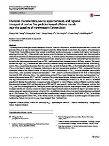
transformation, and deposition of atmospheric pollutants on an urban and regional scale.14 Version 4.3 of CMAQ was the latest available at the time of analysis. It included the third version of the modal aerosol dynamics model and incorporates improved secondary particulate mechanisms, along with the ISORROPIA model,15,16 to process the thermodynamic equilibrium of inorganic aerosol species. This study used the Carbon Bond IV (CB-IV) chemical mechanism. Meteorology inputs were processed using MM5 (a community mesoscale meteorology model developed by the National Center for Atmospheric Research and Pennsylvania State University).17–19 Approach The overall approach consisted of running the CMAQ model with and without the various source categories and analyzing the results to identify the contribution of each. Episode and Modeling Domain The episode that was chosen for this study consisted of 11 days from August 29, 1999, to September 8, 1999. This episode included days with high ozone concentrations in the Tennessee region and was modeled as part of the Arkansas, Tennessee, Mississippi Ozone Study. An analysis of the monthly average PM2.5 concentrations collected at Look Rock, TN, as part of the Interagency Monitoring for Protected Visual Environments (IMPROVE) network showed that the PM2.5 concentrations in 1999 peaked

during the months of July and August, as shown in Figure 2. Although the selected episode was a high ozone episode that occurred at the end of the peak PM2.5 period, it was used for the following reasons. First, secondary PM2.5 formation is partly photochemical in nature, on the basis that most mechanisms that cause secondary PM2.5 formation involve free radicals that are generated by photochemical reactions. Moreover, 24-hr average PM2.5 mass was found to correlate reasonably well with the maximum daily 1-hr average ozone concentrations.20 Second, it is assumed that the episode would still be representative of a typical high PM2.5 season because of the fact that the composition of the individual species seemed to be relatively constant for the selected period. A three-tiered nested domain was used to minimize the effect of boundary conditions. The coarse outer domain consisted of a 36-km by 36-km grid resolution. The intermediate domain consisted of 12-km grid resolution. The innermost domain consisted of 4-km by 4-km grid cells covering the state of Tennessee. Figure 3 shows the modeling domain used for the photochemical modeling using CMAQ. A vertical resolution of 11 layers was configured following the ␴-pressure structure with denser grids at lower levels so as to better resolve the boundary layer. The vertical resolution affects the ability of the model to characterize vertical transport by turbulent mixing and diffusion, plume rise, and the influence of clouds on aerosol chemistry and dynamics. In particular, this may affect the aerosol sulfate processes taking place within the clouds.21 The optimum number and resolution of the vertical layers is a compromise between accuracy and the available time and computing resources. Morris et al.22 tested the sensitivity of the CMAQ model to the number of vertical layers (34 vs. 19). They found that the simulation with 34 vertical layers took 80% more computer processing time than the 19-layer simulation, while showing no definite conclusion as to which simulation was better. Hence, they used the 19-layer resolution in their simulations. Although a larger number of vertical layers might have been preferred, the available resources at the time of the simulation limited the choice to 11 vertical layers in this

Figure 1. Map of counties in Tennessee highlighting nonattainment counties and counties presented in this analysis. 408 Journal of the Air & Waste Management Association

Volume 57 April 2007

Doraiswamy, Davis, Miller, and Fu

Figure 2. Monthly average PM2.5 composition at Look Rock in Tennessee in 1999; EC ⫽ elemental carbon; OC ⫽ organic carbon.

study. Table 2 summarizes the modeling domain parameters used in this study. Emissions Processing Because Tennessee was the region of focus in the highresolution domain (4 km), emissions in Tennessee were estimated by the emissions inventory group at the University of Tennessee (UT). The on-road mobile source emission inventory for Tennessee23 was prepared using EPA’s mobile source emission factor model, MOBILE6. The point source

inventory and ammonia24 emissions inventory for Tennessee were also prepared by UT. EPA’s national emission inventory (NEI) for 1999 was used for area and nonroad mobile source emissions (except ammonia) for Tennessee. For states other than Tennessee, the NEI database was used for all of the source categories. For electric utility plants, data obtained from the continuous emissions monitoring system were used. This enabled the use of actual emissions from power plants in preference to the estimated emissions in the NEI database. The average emissions were processed using the Sparse Matrix Operator Kernel Emissions (SMOKE) model (version 1.4)25 to generate speciated, hourly emissions for each grid cell in the domain. More information is available elsewhere.13,26 Model Application The base case simulation consisted of a run with all of the sources included. The 36-km domain was first modeled. The default set of boundary and initial conditions available in CMAQ was used for the 36-km domain run. The output from the 36-km domain provided the boundary and initial conditions for the 12-km domain, the results of which were then used as boundary and initial conditions for the 4-km domain. Because the first day of the episode under consideration was August 29, 1999, the model runs were set to start 2 days earlier (August 27,

Figure 3. Nested CMAQ modeling domain. Volume 57 April 2007

Journal of the Air & Waste Management Association 409

Doraiswamy, Davis, Miller, and Fu Table 2. Modeling domain parameters.

Parameter 36-km domain dimensions 12-km domain dimensions 4-km domain dimensions

Meteorological Modeling 54 columns, 48 rows 97 columns, 73 rows 208 columns, 76 rows

Vertical resolution 23 layers Y-center (latitude), X-center 35.5o North, 86o West (longitude)

CMAQ Modeling 48 columns, 42 rows 94 columns, 70 rows 205 columns, 73 rows 11 layers 35.5o North, 86o West

1999) to allow for the “spin-up” period. This was to eliminate the influence of the initial conditions on the model results. Once model performance evaluation was completed, different scenarios (Table 3) were modeled to estimate the major source contributions. The difference between the base case concentrations and a specific scenario was considered (with adjustments, as explained later) to be contributed by the source category eliminated in that scenario. RESULTS Base Case Predictions and Model Performance Limited monitoring data were available for this episode for the sites in Tennessee. The average concentration from a 7 ⫻ 7 matrix of grid cells, with the cell containing the monitor at the center, was used for comparing against the measured PM2.5 concentration.27 Figure 4 shows observed and predicted PM2.5 concentrations for a few sites and a scatter plot of data from all of the sites in Tennessee. The model appeared to underpredict for the first half of the episode and overpredict for the second half of the episode. There were ⬃24 monitoring sites in Tennessee that

had some data. Because of the lack of sufficient data to calculate performance metrics for each site individually, the data from all of the sites were analyzed collectively to determine the aggregated metrics. The performance metrics are tabulated in Table 4. On average, the model overpredicted by ⬃8% over the whole episode. The aggregated normalized gross error was 33%. EPA guidance27 recommends that the normalized bias be ⬍20%. The guidance for gross error is ⱕ30% following the ozone guidance measures that EPA has used historically. Seigneur,28 in his review of particulate models, found that the normalized gross error for PM2.5 mass predictions varied from 30% to 50%. This is also reported in the EPA guidance.27 The IMPROVE site at Look Rock, TN, was the only site in Tennessee that had speciation data for the days modeled. The EPA guidance27 also suggests comparing the relative proportions of each constituent species as a percentage of the total PM2.5. Table 5 summarizes the relative percentage of each constituent species as predicted by the model and compares it to the observed (measured) fractions. The guidance recommends that, for the major species (ⱖ30% of total PM2.5), the relative proportion predicted for each component averaged over modeled days with monitored data should agree within ⬃20% of the average observed proportion and that, for the minor species, the data should be within a goal of 5%. As seen, the relative proportion of the major species averaged over days with monitored data was within the stated objective of 20%. It appears that the model overpredicted the ammonium fractions and underpredicted the organic fractions. The overprediction of ammonium fraction might be possibly related to an overestimate of the ammonia emission inventory. Because ammonium is in equilibrium with sulfate and nitrate, another possibility is that it might be associated with the overestimation of sulfate

Table 3. Source apportionment scenarios. Source

Scenario

SCCs Eliminateda

Objective

All

1. All sources present 2. No primary PM

None Not applicable

Base case and identification of primary vs. secondary PM2.5

Coal-fired power plants

Without coal power plants in the domain

101001, 101002, and 101003

Contribution of coal power plants to ambient PM2.5, primary PM2.5 and secondary PM2.5 formation, sulfates, and nitrates

On-road mobile

1. Without on-road mobile sources (exhaust and fugitive) in the whole domain 2. Without exhaust emissions only

2201, 2230, 2294, and 2296

Contribution of mobile source exhaust and fugitive dust to ambient PM2.5

Area sources

Without sources, such as livestock operations and agricultural activities

2801 and 2805

Contribution of NH3 emissions from livestock and agriculture to secondary PM2.5

Nonroad mobile

Without non-road mobile sources in the whole domain

2260, 2265, 2267, 2268, 2270, 2275, 2280, 2282, 2283, and 2285

Contribution of nonroad mobile sources to ambient PM2.5

Pollutant sensitivity runs

No NH3 emissions (all sources with ammonia emissions set to 0)

Not applicable

Sensitivity of NH3 control on PM2.5 vs. NOx and SO2 control

2201 and 2230

Notes: aSource Classification Codes (SCCs) beginning with the listed digits were eliminated. 410 Journal of the Air & Waste Management Association

Volume 57 April 2007

Doraiswamy, Davis, Miller, and Fu

Figure 4. Comparison of model-predicted concentrations to observed values: (a) scatter plot of predicted concentrations vs. observed concentrations for all sites in Tennessee, and (b– e) observed and predicted concentrations for selected sites in Tennessee: (b) Shelby County; (c) Montgomery County; (d) Sumner County; (e) Hamilton County.

and nitrate concentrations. The underprediction of organic fraction might be related to the limitation of the current algorithms to correctly simulate secondary organic aerosol (SOA) fractions. The organic aerosol mechanism is in a mode of continual improvement as new information becomes available.21,29 Morris et al.30 identified several processes that are currently not accounted for in the SOA module in CMAQ, including the following: (1) polymerization of SOA resulting in nonvolatile species; (2) formation of SOA from sesquiterpenes, isoprene, and from biogenic volatile organic compounds (VOCs) other than isoprene and monoterpenes; (3) acid catalyzed reactions of SOA; and (4) SOA Volume 57 April 2007

formation from heterogeneous aqueous-phase chemical reactions. A sensitivity analysis showed that including the effects of SOA polymerization and SOA formation from sesquiterpenes and isoprene reduced the bias (between model predictions and observed concentrations) from ⫺102% to ⫺2% for the Southeastern United States and from ⫺82% to ⫺14% for the Northeastern United States,30 suggesting a significant improvement in model performance compared with the case without the SOA modifications. Considering the inherent uncertainty in these models and the fact that model predictions appeared to track the trend, the model performance was considered satisfactory Journal of the Air & Waste Management Association 411

Doraiswamy, Davis, Miller, and Fu Table 4. Aggregated model performance metrics for PM2.5 for sites in 4-km domain.

Modeled Days in 1999 August 29 to September 8 (all 11 days) August 29 to September 3 (6 days) September 4–8 (5 days)

No. of Data Points

Aggregated Normalized Bias, Ba (%)

Aggregated Normalized Gross Error, Gb (%)

60 40 20

8 ⫺10 45

33 21 58

冉

冊 冊

Predicted ⫺ Observed 1 ¥ ¥ Ntot all monitoring sites days with monitored data Observed 1 Predicted ⫺ Observed b G ⫽ ¥ ¥ ABS Ntot all monitoring sites days with monitored data Observed where Ntot refers to the total number of days (or hours) with paired predictions and observations at all monitoring sites included in the calculation, and ABS refers to the absolute value of the term within parentheses. Notes: aB ⫽

冉

and similar to the performance seen by other researchers.28 Although the model underpredicted the total PM2.5 mass by ⬃10% for the 4-km domain for days before September 4, 1999, and overpredicted for the second half of the episode, its effect on the results should be minimal, because the analysis approach involves considering the difference in mass concentrations between two scenarios rather than the absolute mass concentrations. This assumes that the factors that contributed to the underprediction and overprediction of PM2.5 mass for that period would contribute similarly in all of the scenarios considered in the analysis, causing minimal effect on the differences between the scenarios. Predicted PM2.5 concentrations were typically ⱖ70% of predicted PM10 (PM of aerodynamic diameter of ⱕ10 ␮m) concentrations. Data from the IMPROVE network showed ambient PM2.5-to-PM10 ratios of ⬃77% for August 1999 and 63% for September 1999. On average, the ratio was 70% at Look Rock for the complete year in 1999. The model-predicted ratios were very similar to that measured at Look Rock. Source Apportionment Results Different scenarios were considered for the purpose of conducting a source apportionment. As mentioned earlier, the basic approach consisted of running the CMAQ model without a particular source category and then analyzing the difference between the base case and the run without the particular source category. This assumes that the changes observed in the concentration of the different species were because of the source category considered. In other words, if the concentration of a species

decreased by “x” units, it is assumed that this decrease is directly related to the absence of the particular source category considered. Although this approach was probably valid for most cases, it did introduce some nonlinearity issues, hence, limiting the amount of scenarios that could be considered, as discussed below. This is similar to the synergistic effects demonstrated by Alpert et al.31 in their sensitivity studies. Estimation Technique Issues. An attempt was made to identify the contribution of major source categories, such as coal-fired boilers (i.e., power plants), on-road mobile sources, nonroad mobile sources, and agricultural sources. Once the contribution of each source category was determined (by difference approach), the sum of the individual contributions was subtracted from the base case concentration to determine the source categories that were not quantified (“other sources”) in this study. Pertinent graphs (Figure 5) from Davidson County (see Figure 1) are discussed to illustrate the consequence of this approach. Figure 5 shows the source contributions to ambient nitrate and ammonium concentrations. The graphs show negative values for “other sources.” In other words, the sum of the predicted nitrate contributions from the major source categories exceeded its base case concentrations. Ammonium concentrations behaved similarly. This implies that one or more source categories predicted higher nitrate and ammonium contributions than what may be truly attributed to them. The agricultural source was

Table 5. Observed and predicted relative proportions of constituent species (% of total PM2.5) at Look Rock. September 1, 1999

September 4, 1999

September 8, 1999

Average

Species

Obs. (%)

Pred. (%)

Obs. (%)

Pred. (%)

Obs. (%)

Pred. (%)

Obs (%)

Pred (%)

Sulfate (SO42⫺) Nitrate (NO3⫺) Ammonium (NH4⫹) OC Elemental carbon Rest of species

41.8 n/a n/a 20.3 2.8 n/a

32.3 3.5 13.1 15.2 1.6 34.2

33.5 0.7 7.5 24.9 3.9 29.9

40.9 2.3 15.8 12.4 1.5 27.3

42.8 0.7 12.0 14.2 2.3 28.2

56.7 0.3 17.2 7.4 1.0 17.4

39.3 0.7 9.8 19.8 3.0 29.0

43.3 1.3 16.5 11.7 1.4 22.4

Notes: n/a ⫽ data not available and predicted fractions for these species on this day was not included in the average; Obs ⫽ observed; Pred ⫽ predicted. 412 Journal of the Air & Waste Management Association

Volume 57 April 2007

Doraiswamy, Davis, Miller, and Fu

Figure 5. Source contributions to (a) nitrate and (b) ammonium at Davidson County with agricultural sources included.

clearly one of them based on the following theory. Agricultural sources accounted for ⬎85% of ammonia emissions. Hence, when the agricultural source category is eliminated, it is equivalent to reducing the ammonia emissions to a negligible value (compared with the base case emissions). This consequently affected the ammonianitric acid equilibrium. Ammonium nitrate could be formed through one of the following reactions (eqs 1 and 2), depending on the ambient relative humidity (RH) and whether it is above or below the deliquescence RH (DRH).15,16,32 This determines whether the aerosol is in a solid state or an aqueous state. At ambient RH above DRH: NH 3共g兲 ⫹ HNO3共g兲 N NH4 ⫹ ⫹ NO3 ⫺

(1)

At ambient RH below DRH: NH 3共g兲 ⫹ HNO3共g兲 N NH4NO3共s兲

(2)

The gas phase should be supersaturated with ammonia and nitric acid (gas phase) for the equilibrium to shift toward the formation of aerosol nitrate. Hence, elimination of ammonia emissions inhibits the formation of aerosol nitrate. This Volume 57 April 2007

was confirmed by a sensitivity run eliminating ammonia emissions from all sources. Thus, any nitrogen oxide (NOx) or nitric acid vapor arising from sources such as on-road mobile, power plants, and so forth that typically would have formed nitrates in the presence of ammonia was probably inhibited and did not transform completely to particulate nitrate. Consequently, when the difference between the base case and the scenario is attributed to agricultural sources, all such inhibited nitrates would also be included in that contribution. As a result, the predicted contribution of agricultural sources to nitrates may include some contributions of other sources of NOx. Hence, the sum of the individual source contributions (mobile ⫹ point ⫹ nonroad ⫹ agricultural) is greater than the base case because of nonlinear effects. For this reason, the contribution of agricultural sources was not quantified separately and was included with the “other sources” category. Source Apportionment Adjustment: Ammonium Allocation. The difference in species concentrations between the base case and a particular scenario may not always be a direct contribution of the source category considered. Figure 6 presents an example for Knox County (see Figure 1). It shows the difference in the 24-hr average PM2.5 concentration between the base case and two different scenarios: “no on-road mobile exhaust” and “no external combustion coal Journal of the Air & Waste Management Association 413

Doraiswamy, Davis, Miller, and Fu

Figure 6. Difference between base case and selected scenarios: (a) “no on-road mobile exhaust” and (b) “no external combustion coal-fired boilers.” EC ⫽ elemental carbon; ORGB ⫽ biogenic organics; ORGA ⫽ secondary anthropogenic organics; ORGPA ⫽ primary anthropogenic organics.

fired boilers.” This difference represents the quantity by which the concentrations changed because of the elimination of emissions from the respective source categories. It must be noted that, whereas the graphs (Figures 6 and 7)

show significant amounts of ammonium concentrations associated with “no exhaust emissions” and with “no coal-fired boilers,” the ammonia emissions from these source categories are negligible. Clearly, this is because of reaction equilibrium.

Figure 7. Percent contribution of source categories to particulate ammonium concentration. 414 Journal of the Air & Waste Management Association

Volume 57 April 2007

Doraiswamy, Davis, Miller, and Fu It must be pointed out that, in recent years, selective catalytic reduction (SCR) and selective noncatalytic reduction (SNCR) technologies are being implemented to control NOx emissions from power plants, which may result in an increase in the ammonia emissions, depending on the system design and the rate of ammonia slippage. However, during the period of study (1999), none of the power plants in the area were equipped with SCR or SNCR systems, and, therefore, ammonia emissions from power plants were negligible. Thus, whereas coal-fired boilers (from power plants) did not emit ammonia as a pollutant, the ammonia emitted by other sources was dependent on the sulfur dioxide (SO2) and NOx emissions from the coal-fired boilers to form PM. As shown by the modeling, the absence of these power plant emissions also reduced the ability of the ammonia to form and be a part of the PM. Thus, indirectly, the coal-fired boilers are responsible for a large fraction (⬃67% on average) of the ammonium particulate formation (Figure 7). Similarly, the on-road exhaust emissions, which contain NOx, accounted for ⬃14% of the ammonium particulate formation (Figure 7). Although the observed differences in ammonium concentrations indicate an indirect contribution, it would be inappropriate to allocate the actual difference in ammonium concentrations to these source categories, when their ammonia emissions (precursor to ammonium formation) are negligible. Hence, in this study, an adjustment was made to the predicted differences in ammonium concentrations based on the emission contribution by the respective source categories. Based on the emission inventory, it was noted that the on-road mobile sources accounted for only 5% of the ammonia emissions in the 36-km domain. Even further, the coal-fired electric generating units accounted for ⬃0.4% and nonroad mobile sources, ⬃0.7% of the ammonia emissions. Hence, of the actual predicted ammonium contribution, only 5% was allocated to on-road mobile exhaust, 0.4% to coal-fired power plants, 0.7% to nonroad mobile sources, and the rest to “other ammonia sources.” Source Contributions at Major Regions in TN. The results are summarized for the four urban regions in Tennessee, namely Knox, Hamilton, Davidson, and Shelby counties and one rural region of Lawrence County (see Figure 1 for locations). Figure 8 shows the complete source apportionment results for each day in the episode for the five regions considered in the analysis. The contribution of the source categories differed from day to day, depending on a variety of factors, including the emissions of local sources and meteorological factors, such as the dominant wind direction. Certain days were dominated by coal-fired boilers, whereas others were dominated by on-road mobile sources. For example, an analysis of the meteorological data from McGhee Tyson Airport, the station closest to Knox County, shows that the dominant direction from which the wind blew was north-northeast (⬃27% of the time) from August 29, 1999, to September 3, 1999 (Figure 9a), while being from the north (⬃11%) and northwest (⬃11%) from September 4 to September 8, 1999 (Figure 9b). Stagnant (“calm”) wind conditions prevailed for 37.5% of the Volume 57 April 2007

time between August 29, 1999, and September 3, 1999, and 48.7% of the time during September 4 – 8, 1999. The day-to-day variation in source contributions could probably be attributed to such differences in meteorological factors, which determine the extent of longrange transport, formation of secondary particles, and dispersion of particles in the air. Stagnant (calm) wind conditions could increase the effect of local sources. Such effects have been observed by others.33,34 Figure 10 shows the mean source contributions over the whole episode. The coal-fired external combustion boilers formed the major source category. Their contribution ranged from 29% to ⬃39%. The higher end was predicted at the rural Lawrence County. On average, the on-road mobile source exhaust emissions contributed from ⬃8 to 9% of the ambient PM2.5 (⬃2 to 3.5 ␮g/m3) at all of the regions considered. The fugitive dust on paved and unpaved roads contributed from ⬃9 to 15%, (⬃2.5 to 4 ␮g/m3) with the lower end predicted at the rural Lawrence County. Thus, of the mobile source contribution, fugitive emissions formed the major fraction, ranging from ⬃53% to 64% of the on-road mobile source contribution. Similar percentages of mobile source contributions have been reported by other studies.5,6,11 Mysliwiec and Kleeman11 estimated the mobile source contribution to be ⬎30% of the total PM2.5 mass in the California region. Receptor modeling conducted by Lewis et al.6 showed that the mobile source contributed ⬃52% of the total PM2.5 mass in the Phoenix, AZ, area. Lee et al.5 reported mobile source contributions of ⬃40% of the fine particle mass in the Toronto region of Canada. The nonroad mobile sources contributed from ⬃3 to 6%. The unidentified source categories (“other sources”) still composed from 22 to 29% of the ambient fine particle concentration. The “other ammonia” sources consists of the adjusted ammonium concentrations as described earlier. This would probably include most ammonia sources that contributed to the predicted ammonium concentrations. This category composed from ⬃13 to 15% of the PM2.5 concentration. An insight into the fine particle composition of the various source contributions would be useful in formulating control policies. The relative fractions of the various species contributed by the sources were similar for the five regions analyzed. For illustration purposes, Figure 11 shows the predicted composition of PM2.5 contributions from each source category for Knox County. The fine particles contributed by the exhaust emissions from on-road mobile sources consisted of sulfates, nitrates, traces of organics, and unspeciated PM2.5. Thus, ⬃75% of the fine particles contributed by on-road mobile exhaust consisted of secondary fractions. The major species that composed fugitive dust contributions was unspeciated primary PM2.5 (⬃95%). The contribution from coal-fired power plants consisted of mainly sulfates and a small fraction of nitrates. Thus, the contributions from power plants are almost entirely secondary in nature. The contribution from nonroad mobile sources was predicted to consist of nitrates and elemental carbon with traces of sulfates and organics, thus making an approximately equal split between primary and secondary fractions. The “other ammonia sources” consist of the adjusted ammonium concentrations as described earlier. This would Journal of the Air & Waste Management Association 415

Doraiswamy, Davis, Miller, and Fu

Figure 8. Source apportionment of PM2.5 at: (a) Knox County, (b) Hamilton County, (c) Lawrence County, (d) Davidson County, and (e) Shelby County.

include most ammonia sources that contributed to the predicted ammonium concentrations. Approximately 10% of the unidentified PM2.5 (“other sources”) is estimated to be biogenic organic carbon, ⬃31% to be other secondary fractions, and the rest of the contribution by “other sources” to be primary in nature. Based on the inventory, the possible source categories of primary PM2.5 would be agricultural sources, industrial processes, and waste disposal and treatment. Possible sources of secondary fractions, in addition to biogenic sources, would include industrial processes and other combustion boilers not considered earlier. This would include numerous individual source categories with relatively smaller emissions compared with the categories included in this study. 416 Journal of the Air & Waste Management Association

DISCUSSION Based on the results presented, the coal-fired power plants are a major contributor to the ambient PM2.5 concentrations, particularly to the sulfates. If the peak summertime fine particle concentrations are to be reduced, it is obvious that the sulfate concentrations need to be reduced. This implies that a reduction in SO2 emissions, the precursor to sulfate formation, is necessary. It must be noted that the results presented in this paper are for the year 1999. With initiatives such as the Clean Air Interstate Rule, it is likely that the SO2 emissions in the future would be more controlled. With sulfate being a secondary pollutant, controlling SO2 emissions in only plants that are in the vicinity of a Volume 57 April 2007

Doraiswamy, Davis, Miller, and Fu

(a)

NORTH

30% 24% 18% 12% 6% WEST

EA ST

SOUTH

NORTH

(b) 15% 12% 9% 6% 3% WEST

EA ST

WIND SPEED (m/s) >= 10.0 8.0 - 10.0 6.0 - 8.0 4.0 - 6.0 2.0 - 4.0

SOUTH

0.5 - 2.0 Calms: 48.65%

Figure 9. Wind rose for McGhee Tyson airport (station closest to Knox County) during: (a) August 29 – September 3, 1999, and (b) September 4 – 8, 1999.

county does not produce a significant reduction in PM2.5 concentration in that county. A region-wide reduction in SO2 emissions would likely be needed to produce beneficial results. The second major source category was estimated to be on-road mobile sources, of which more than half originated from fugitive dust on roads. With various regulations (such as the heavy-duty engine NOx controls and fuel sulfur regulations) in effect, the precursors to secondary particle formation will be controlled, and the exhaust emissions of NOx, Volume 57 April 2007

VOC, SO2, PM2.5, and PM10 from on-road mobile sources are projected to decrease in the future.23,35 Although the ammonia emissions (which are a precursor to the ammonium component of PM) from on-road mobile sources in Tennessee are projected to increase in the future (⬃6% between 1999 and 2030),35 they are still a small fraction (4% in 1999) of the overall ammonia emission inventory to cause a significant increase in secondary particle formation. Thus, for on-road mobile sources, the relative contribution of primary PM may Journal of the Air & Waste Management Association 417

Doraiswamy, Davis, Miller, and Fu

Figure 10. Predicted mean source apportionment of PM2.5.

increase in the future. Hence, in the future, the relative fraction of fugitive dust may be even greater than that estimated in this study. With all of the other factors remaining constant, the on-road mobile source emissions are a direct function of the vehicle miles traveled (VMTs). This illustrates the importance of reducing the rate of increase in VMTs. Such controls are voluntary in nature and are exercised through public education and awareness. For example, on days that are forecast to be high-ozone days (“ozone-action days”), local governments request citizens to consider limiting the number of vehicle trips (which translate into VMT) or to combine errands to reduce driving. This could similarly be implemented for days forecasted to be high-PM2.5 days (“PM2.5 action days”). It was estimated that the agricultural sources are likely to be a major source given the magnitude of their primary PM2.5 emissions and ammonia emissions. Research on emissions from livestock and other feedlot operations are relatively recent. With more data likely being available in the future, it would provide the scientific community with additional information needed to further address the contribution from ammonia-based emissions.

CONCLUSIONS AND RECOMMENDATIONS Overall, the coal-fired external combustion boilers contributed from ⬃39 to 51% of the 24-hr average PM2.5 concentration. The on-road mobile sources contributed from ⬃19 to 26%, with approximately a 60:40 split between fugitive and exhaust contributions. The nonroad mobile sources contributed from ⬃3 to 6% of 24-hr average PM2.5. The results indicate that the source contributions varied day to day. On average, the source contributions were similar at the major regions in Tennessee. The model results are bound by the uncertainties involved in the inventory, chemical mechanisms, and the current understanding of the chemistry, initial and boundary conditions, and so on. The chemical mechanisms are in a continual mode of improvement. The organic aerosol mechanisms are one such where modifications are being done as a better understanding of the chemistry becomes available. Moreover, the predicted composition of primary species is dependent on the speciation profiles in the inventory processor, which again needs to be updated as and when new information becomes available. However, even with all of the limitations, the results give an insight into the major source

Figure 11. Predicted composition of source contributions at Knox County, TN (ORGPA ⫽ primary anthropogenic organics; ORGA ⫽ secondary anthropogenic organics; ORGB ⫽ biogenic organics; EC ⫽ elemental carbon). 418 Journal of the Air & Waste Management Association

Volume 57 April 2007

Doraiswamy, Davis, Miller, and Fu categories and the pollutants that are responsible. Although the results presented in this study are based on an episode during the summer season for the year 1999, the summertime source contribution estimates provided may still be representative of annual contributions, because the annual concentrations are dominated by the summer period concentrations. However, fine particle composition varies over the season for the southeastern part of the United States, based on data from the IMPROVE network, implying differences in seasonal contributions. An insight into the seasonal contributions might serve as a useful policy tool in determining the most optimal source control strategies. Hence, more modeling is recommended for other seasons of the year to determine the seasonal source contributions. ACKNOWLEDGMENTS The authors acknowledge the Tennessee Department of Transportation for funding this study in part and the Air Pollution Control Division of Tennessee Department of Environment and Conservation for providing Federal Reference Method PM2.5 data. Sincere thanks are also due to the IMPROVE network for providing the speciation data and to the atmospheric sciences group at the Tennessee Valley Authority for allowing us to use the data from the Tennessee Valley PM2.5 Special Purpose Monitoring Network. REFERENCES 1. Klemm, R.J.; Mason, R.M., Jr.; Heilig, C.M.; Neas, L.M.; Dockery, D.W. Is Daily Mortality Associated Specifically with Fine Particles? Data Reconstruction and Replication of Analyses; J. Air & Waste Manage. Assoc. 2000, 50, 1215-1222. 2. Watson, J.G. Visibility: Science and Regulation; J. Air & Waste Manage. Assoc. 2002, 52, 628-713. 3. Slater, J.F.; Dibb, J.E.; Keim, B.D.; Talbot, R.W. Light Extinction by Fine Atmospheric Particles in the White Mountains Region of New Hampshire and Its Relationship to Air Mass Transport; Sci. Total Environ. 2002, 287, 221-239. 4. National Air quality and Emissions Trends Report, 1999; EPA 454/R-01-004; U.S. Environmental Protection Agency: Research Triangle Park, NC, 2001. 5. Lee, P.K.H., Brook, J.R.; Dabek-Zlotorzynska, E.; Mabury, S.A. Identification of the Major Sources Contributing to PM2.5 Observed in Toronto; Environ. Sci. Technol. 2003, 37, 4831-4840. 6. Lewis, C.W.; Norris, G.A.; Conner, T.L.; Henry, R.C. Source Apportionment of Phoenix PM2.5 Aerosol with the Unmix Receptor Model; J. Air & Waste Manage. Assoc. 2003, 53, 325-338. 7. Maykut, N.N.; Lewtas, J.; Kim, E.; Larson, T.V. Source Apportionment of PM2.5 at an Urban IMPROVE Site in Seattle, Washington; Environ. Sci. Technol. 2003, 37, 5135-5142. 8. Gertler, A.W.; Gillies, J.A.; Pierson, W.R. An Assessment of the Mobile Source Contribution to PM10 and PM2.5 in the United States; Water Air Soil Pollut. 2000, 123, 203-214. 9. National Research Council. Research Priorities for Airborne Particulate Matter: II—Evaluating Research Progress and Updating the Portfolio; National Academy Press: Washington, DC, 1999 10. Kleeman, M.J.; Hughes, L.S.; Allen, J.O.; Cass, G.R. Source Contributions to the Size and Composition Distribution of Atmospheric Particles: Southern California in September 1996; Environ. Sci. Technol. 1999, 33, 4331-4341. 11. Mysliwiec, M.J.; Kleeman, M.J. Source Apportionment of Secondary Airborne Particulate Matter in a Polluted Atmosphere; Environ. Sci. Technol. 2002, 36, 5376-5384. 12. Pun, B.K.; Wu, S.Y.; Seigneur, C. Contribution of Biogenic Emissions to the Formation of Ozone and Particulate Matter in the Eastern United States; Environ. Sci. Technol. 2002, 36, 3586-3596. 13. Doraiswamy, P. Ph.D. Dissertation, University of Tennessee, Knoxville, TN, December 2004. 14. Byun, D.W.; Ching, J.K.S. Science Algorithms of the EPA MODELS-3 Community Multiscale Air Quality (CMAQ) Modeling System; EPA/600/R99/030; Office of Research and Development, U.S. Environmental Protection Agency: Washington, DC, 1999. 15. Nenes, A.; Pandis, S.N.; Pilinis, C. ISORROPIA: a New Thermodynamic Equilibrium Model for Multiphase Multicomponent Inorganic Aerosols; Aquatic Geochem. 1998, 4, 123-152. Volume 57 April 2007

16. Nenes, A.; Pandis, S.N.; Pilinis, C. Continued Development and Testing of a New Thermodynamic Aerosol Module for Urban and Regional Air Quality Models; Atmos. Environ. 1999, 33, 1553-1560. 17. Dudhia, J.; Bresch, J.F. A Global Version of the PSU-NCAR Mesoscale Model; Mon. Weather Rev. 2002, 130, 2989-3007. 18. Dudhia, J.; Gill, D.; Guo, Y.R.; Hansen, D.; Manning, K.; Wang, W. PSU/ NCAR Mesoscale Modeling System Tutorial Class Notes (MM5 Modeling System Version 2); National Center for Atmospheric Research: Boulder, CO, 1998. 19. Grell, G.A.; Dudhia, J.; Stauffer, D. A Description of the Fifth-Generation Penn State/NCAR Mesoscale Model (MM5). NCAR Technical Note, TN-398 ⫹ STR; National Center for Atmospheric Research: Boulder, CO, 1994. 20. Parkhurst, W.J.; Tanner, R.L.; Weatherford, F.P.; Valente, R.J.; Meagher, J.F. Historic PM2.5/PM10 Concentrations in the Southeastern United States—Potential Implications of the Revised Particulate Matter Standard; J. Air & Waste Manage. Assoc. 1999, 49, 1060-1067. 21. Binkowski, F.S.; Roselle, S.J. Models-3 Community Multiscale Air Quality (CMAQ) Model Aerosol Component 1. Model Description; J. Geophys. Res. 2003, 108, AAC 3-1–AAC 3-18. 22. Morris, R.E.; Koo, B.; Lau, S.; Tesche, T.W.; McNally, D.; Loomis, C.; Stella, G.; Tonnesen, G.; Wang, Z. VISTAS Emissions and Air Quality Modeling—Phase I Task 4cd Report: Model Performance Evaluation and Model Sensitivity Tests for Three Phase I Episodes; ENVIRON International Corporation, Alpine Geophysics LLC and CE-CERT of University of California, Riverside: Riverside, CA, 2004. 23. Davis, W.T.; Miller, T.L.; Reed, G.D.; Tang, A.M.Y.; Doraiswamy, P.; Sanhueza, P. Effects of Growth in VMT and New Mobile Source Emission Standards on NOx and VOC Emissions in Tennessee, 1999 –2030 (Based on Mobile6-Final Version); The University of Tennessee: Knoxville, TN, 2002. 24. Kim, Y. M.S. Thesis, The University of Tennessee, Knoxville, TN, May 2003. 25. MCNC Environmental Modeling Center. Sparse Matrix Operator Kernel Emissions (SMOKE) Modeling System Version 1.4.2. User Manual; MCNC Environmental Modeling Center (now with Carolina Environmental Program at the University of North Carolina at Chapel Hill): Chapel Hill, NC, 2002. 26. Doraiswamy, P.; Davis, W.T.; Miller, T.L.; Fu, J.S. Contribution of On-road Mobile Sources to PM2.5 in Tennessee; In Proceedings of A&WMA’s 97th Annual Conference & Exhibition, Pittsburgh, PA, June 22–25, 2004; Paper 112. 27. Draft Guidance for Demonstrating Attainment of Air Quality Goals for PM2.5 and Regional Haze; U.S. Environmental Protection Agency: Research Triangle Park, NC, 2001. 28. Seigneur, C. Current Status of Air Quality Models for Particulate Matter; J. Air & Waste Manage. Assoc. 2001, 51, 1508-1521. 29. Schell, B.; Ackermann, I.J.; Hass, H.; Binkowski, F.S.; Ebel, A. Modeling the Formation of Secondary Organic Aerosol within a Comprehensive Air Quality Model System; J. Geophys. Res. 2001, 106, 28275-28293. 30. Morris, R.E.; Koo, B.; Guenther, A.; Yarwood, G.; McNally, D.; Tesche, T.W.; Tonnesen, G.; Boylan, J.; Brewer, P. Model Sensitivity Evaluationfor Organic Carbon Using Two Multi-Pollutant Air Quality Models That Simulate Regional Haze in the Southeastern United States; Atmos. Environ. 2006, 40, 4960-4972. 31. Alpert, P.; Tsidulko, M.; Stein, U. Can Sensitivity Studies Yield Absolute Comparisons for the Effects of Several Processes?; J. Atmos. Sci. 1995, 52, 597-601. 32. Seinfeld, J.H.; Pandis, S.N. Atmospheric Chemistry and Physics: from Air Pollution to Climate Change; John Wiley & Sons: New York, NY, 1998. 33. Elminir, H.K. Dependence of Urban Air Pollutants on Meteorology; Sci. Total Environ. 2005, 350, 225-237. 34. Mossetti, S.; Angius, S.P.; Angelino, E. Assessing the Impact of Particulate Matter Sources in the Milan Urban Area; Int. J. Environ. Pollut. 2005, 24, 247-259. 35. Yun, J. M.S. Thesis, The University of Tennessee, Knoxville, TN, August 2004.

About the Authors Prakash Doraiswamy, formerly of the University of Tennessee, is currently a postdoctoral research associate with the State University of New York–Albany. Wayne Davis is a professor and associate dean for research at the University of Tennessee at Knoxville, TN. Terry Miller is an associate professor, and Joshua Fu is a research assistant professor in the Department of Civil and Environmental Engineering at the University of Tennessee. Address correspondence to: Wayne T. Davis, College of Engineering, 124 Perkins Hall, University of Tennessee, Knoxville, TN 37996; phone: ⫹1-865-974-5321; fax: ⫹1-865-974-8890; e-mail: [email protected].

Journal of the Air & Waste Management Association 419