Aug 2, 2002 - adapted source code transformations can improve Grid application ... and storage resources, network based computing will soon offer to users ...
TAG research report LSIIT-ICPS Pôle API, Bd. S. Brant F-67400 Illkirch
August 2, 2002
Source Code Transformations Strategies to Load-balance Grid Applications Romaric David, Stéphane Genaud, Arnaud Giersch, Benjamin Schwarz, and Eric Violard {david,genaud,giersch,schwarz,violard}@icps.u-strasbg.fr Tel: +33 3 90 24 45 42 / Fax: +33 3 90 24 45 47
August 2, 2002 Abstract We present load-balancing strategies to improve performances of parallel MPI applications running in a Grid environment. We analyze the data distribution constraints found in two scientific codes and propose adapted code transformations to load-balance computations. We present the general framework for our load-balancing techniques. We then describe these techniques as well as their application to our examples. Experimental results confirm that adapted source code transformations can improve Grid application performances.
1
Introduction
With the growing popularity of middle-ware dedicated at making so-called Grids of processing and storage resources, network based computing will soon offer to users a dramatic increase in the available aggregate processing power. The end-user will benefit from such a computing power only if new tools are made available to ease the use of such computing resources. Traditionally, many scientific applications have been developed by users with a parallel computer in mind. Users are thus used to work on a single host with a single-image file system and most of the time, a unique memory space (even if it is physically distributed). Furthermore, the parallel code is designed assuming an homogeneous set of processors with homogeneous and very high bandwidth links between processors. All these features that make the user comfortable with the system disappear with clusters or Grids. There are numerous difficulties that should be overcome to make the use of Grids more popular. One of the major difficulties lies in the poor performances obtained with most parallel applications when run on a Grid. There are two major reasons for the lack of performance: first, the processors available are heterogeneous and hence the work assigned to processors is often unbalanced, and secondly the network links are orders of magnitude slower on the Grid than in a parallel computer. Much work has been carried out to take into account such heterogeneous environments for distributed computing: these efforts range from the optimization of communication libraries to the migration of processes to balance processors load. Among these techniques, load-balancing is certainly one of the most useful. Studies on load-balancing generally consider the running processes and the physical resources they use, to decide how to load-balance (e.g. [BGW93]). Less often, load-balancing code is included into the application source code itself so as to improve performance in some particular cases (e.g. [SWB98]). However, few research works concern loadbalancing strategies specifically guided by the application to be run. The well-known AppLeS project [BWF+ 96] uses information drawn from a specific application to schedule the execution of the application processes, but they do not modify the application source code to improve its execution. Thus, our project is original in the sense that we study how source code transformations may impact on the performances obtained when running applications on Grids, and
2
3
LOAD-BALANCING FOR UNCONSTRAINED DATA DISTRIBUTION
eventually systematically operate these transformations so as to produce programs permanently adapted to heterogeneous environments. To validate our ideas, we work on some real scientific applications written with MPI. This paper presents preliminary results concerning load-balancing techniques we designed and implemented to improve performances of two scientific applications. We analyze the constraints inherent to the applications and propose adapted code transformations to load-balance computations. The paper is organized as follows: the first section explains the general framework for our load-balancing strategies and the two following sections describe the two test applications. For each application, we first explain its requirements, which load-balancing may be used and under which hypotheses. We finish the sections with experimental results. The last section comments on the code transformations operated and discusses future work.
2
Study framework
Our work is part of the TAG project1 which aims at proposing tools for the end user so as to improve the usability of Grids. One important step to reach this goal is to identify the key characteristics of Grid applications in order to design techniques that would enable to write parallel applications optimized for a Grid environment. In this study, we have rewritten some parts of the tested applications to introduce load-balancing. Load-balancing is a natural way to address the problems arising when working in an heterogeneous environment. Many research works have been conducted in this domain, the greater part of which usually discern two strategies: static load-balancing and dynamic load-balancing [KK92]. Static load-balancing attempts to determine appropriate shares of work to distribute to processors at application startup, while dynamic load-balancing may redistribute part of the work during the execution to compensate for differences in processors performance. In our work, we try to consider both alternatives and assess which would be more profitable depending on the application type. Our study is limited to SPMD applications using a message passing programming model. To validate our ideas, we work on real programs such as the two scientific applications presented as motivating examples in the two next sections. The two applications differ by their data distribution constraints, and we have to encompass how this impacts on the load-balancing strategies to apply. The first application belongs to the so-called embarrassingly parallel class of applications, which means that data distribution is unconstrained: it is possible to send any chunk of data to any process. On the contrary, the second application exhibits data dependencies and hence the data distribution is constrained. These two different data distribution constraints motivated two distinct load-balancing answers detailed in the next two sections: • for unconstrained data distribution, we propose modifications of the source code to allow a direct data repartition accordingly to the processors and network links speeds, • for constrained data distribution, we propose a load-balancing technique consisting in emulating real MPI processes: on each machine the transformed code simulates the execution of more or less processes depending on the processors speed.
3
Load-balancing for unconstrained data distribution
3.1
Motivating example: a geophysical application
We consider for our first experiment a geophysical code in the seismic tomography field. For our purpose, we only need to roughly sketch one part of the application structure. The input data is a set of seismic waves, each described by a pair of 3D coordinates (the coordinates of the seism source and those of the receiving captor) plus the wave type. With these characteristics, a seismic wave can be modelized by a set of ray paths, that represents the wavefront propagation. Seismic 1 TAG
stands for Transformations and Adaptations for the Grid (http://grid.u-strasbg.fr/).
3
TAG project
3
LOAD-BALANCING FOR UNCONSTRAINED DATA DISTRIBUTION
wave characteristics are sufficient to perform the ray-tracing of the whole associated ray path. Hence, all ray paths can be traced independently. It is also important to note that the ray-tracing of the various ray paths require a varying amount of computations. The parallelization of the application, presented in [GGM02], assumes that all available processors are homogeneous (the implicit target for execution is a parallel computer). The following pseudo-code outlines the main communication and computation phases: if (rank = ROOT) raydata ← read n lines from data file; MPI_Scatter(raydata, n/P , ..., rbuff, ..., ROOT,MPI_COMM_WORLD); compute_work(rbuff);
where P is the number of processes involved. The MPI_Scatter instruction is executed by the root process and the computation processes. In MPI, this primitive means that the process identified as ROOT performs a send of distinct blocks of n/P elements from the raydata buffer to all processes of the group while all processes make a receive operation of their respective data in the rbuff buffer. Figure 1 shows a potential execution of this communication operation, with p1 as root process. p1
p2
p3 t0
computing idle actually sending or receiving
time
t1
Figure 1: A scatter communication followed by a computation phase.
From this existing implementation, we now examine which transformations would be profitable for the execution on a Grid. We can quickly think of two manners of load-balancing this kind of application: • The first one is dynamic: a classical master/slave scheme is a good candidate solution for such an heterogeneous environment. In this case, one master process reads small chunks of the input data set and distributes these chunks to slave processes, which compute the received piece of data. As soon as a slave process has finished its computations, it asks the master for a new chunk. The process repeats until the master sends a termination message to slaves. • The second one is static: much like the above pseudo-code, the root process distributes the whole data set in a single communication round, except that it sends unequal shares of data whose sizes are statically computed on the basis of the processors and network performances. We have implemented and tested both program transformations, and are particularly interested in comparing them in terms of performance but also in terms of code rewriting. As far as automatic program transformation is concerned, the second technique is more interesting, since MPI provides a MPI_Scatterv primitive that allows such irregular data distribution and hence the program transformation is more direct. Thus, we focus in our study on the conditions the application must meet to implement this load-balancing technique, and which performance results can be obtained with it.
4
TAG project
3
LOAD-BALANCING FOR UNCONSTRAINED DATA DISTRIBUTION
3.2
Hypotheses for unconstrained data distribution
The static load-balancing technique applies for SPMD programs (also refered to as data-parallel MPI programs [Geo99]) that contain communication-computation phases. A communicationcomputation phase is characterized by a round of simultaneous communications between all processes, followed by local computations ended by a global synchronization —that is an explicit barrier or a synchronization through a second communication round. Note that programs which follow the Bulk Synchronous Programming model [Val90] are entirely build with successive such phases. In the particular case of the geophysical application presented above, there is only one major communication-computation phase and only one process sends the whole input data set to other processes. Moreover, we must state further assumptions the programmer must verify before the load-balancing may take place. (H1) The data items in the input data set are independent. (H2) The number of data-items is the only factor in time complexity. Hence, giving any equal-size part of the domain to a given process will result in the same computation time.
3.3
Static load-balancing of computations and communications
We now introduce some basic metrics to compute the load-balancing: we need a metric to measure the time spent in a computation phase on a given processor during a given period, and a metric to evaluate the time spent to send a given volume of data during a given period. Given the changing state of network links and processors loads, we can ignore the periods at which events occur by using average values for computation and communication speeds. Our metrics thus only depend on data size. For a given communication-computation phase, we define: • compi (d) to be a continuous increasing function that returns the mean time needed to compute d data items on a processor pi and, • commi (d) to be a continuous increasing function that returns the mean time spent in communication for d data items on a processor pi . Our objective is to minimize the elapsed time between the synchronization points (t1 − t0 on figure 1). Assuming (H2)2 , a process pi among P processes should receive a share of di (di ∈ N , i ∈ [1, P ]) data items from the dataset of size D, such that: max{compi (di ) + commi (di ) | i ∈ [1, P ] and
P X
di = D}
(1)
i=1
is minimum. With these notations, the following problem formulation: � comm1 (d01 ) + comp1 (d01 ) = · · · = commP (d0P ) + compP (d0P ) d01 + d02 + · · · + d0P = D
(2)
for which we search for the d0i ∈ R, implies that the di = round(d0i ) satisfy equation (1), where the function round appropriately rounds the real values d0i . This round process is described in Appendix B.2.
3.4
Load-balancing scatter operations
When the communication round is a scatter operation (as in our test application), we can precise the communication cost function and define it as the affine function: commi (d) = bi · d + li , where bi and li are the network bandwidth and latency (resp.) from root processor to processor pi . 2 Note that without (H2) the problem would be far more complex: we would have to build all partitions of the data set in P subsets, and for each subset, evaluate the time of all the permutations from subsets to processors.
5
TAG project
3
LOAD-BALANCING FOR UNCONSTRAINED DATA DISTRIBUTION
Moreover, (H2) implies that the computation cost function compi is linear with the number of data items so we can let compi be a linear function: compi (d) = ai · d. Therefore, equation (2) can be written as the following linear system: � (a1 + b1 ) · d1 + l1 = (a2 + b2 ) · d2 + l2 = · · · = (aP + bP ) · dP + lP d1 + d2 + · · · + dP = D For shortness, let us define ci = ai + bi and T = c1 · d1 + l1 . We thus write � c1 · d1 + l1 = c2 · d2 + l2 = · · · = cP · dP + lP d1 + d2 + · · · + dP = D For each i we can then write di =
T −li 3 , ci
which leads to D =
And then have a general expression for T : T =
PP
i=1
T −li ci
=T×
PP
1 i=1 ci
−
PP
li i=1 ci
P li D+ P i=1 ci PP 1 i=1 ci
From this we can extract a general expression for di : D+ di =
PP li lj j=1 cj j=1 cj − PP ci · ( j=1 c1j )
PP
(3)
Hardware model We must refine this expression with further assumptions on the networking capabilities of the nodes. We consider the full overlap, single-port model of [BCF+ 01] in which a processor node can simultaneously receive data, send data to at most one destination (full-duplex network cards), and perform some computation. This model has shown to be realistic in our experiments, and is representative of a large class of modern machines. As the root process sends data to processes in turn4 a receiving process actually begins its communication after all previous processes have been served. The root process starts its computation after all the processes have received their data. This leads to a “stair effect” represented on figure 1 by the end times of the receive operations (black boxes). We call the delay during which a process pi waits for the communication to actually begin, the startup time, noted si . If we let the root process be p1 , si is defined as: s2 = k si = si−1 + bi−1 · di−1 (i ∈ [3, P ]) s1 = sP + bP · dP where k is a system overhead incurred by the preparation of data to be sent by the root process. The startup time should be integrated as part of the latency parameter (li ) in equation (3). The resolution becomes however not trivial because di depends on d1 , . . . , dP . A means to circumvent the PP problem is to omit, in a first instance, the latency to compute some initial di = D/(ci · j=1 c1j ). From these results we can approximate the startup times. These startup times can then be cumulated to latency to compute the final di .
3.5
Experimental results
Our experiment consists in the computation of 827,000 ray paths on 16 processors. Processors are located at two geographically distant sites. All machines run Globus [FK97] and we use MPICHG2 [FK98] as message passing library. Table 1 shows the resource repartition across sites as well as the processors relative ratings. These ratings come from a series of benchmarks we performed on 3 This 4 In
expression as well as the following one are correct because the ci are strictly positives. the MPICH implementation, the order of the destination processes in scatter operations follows the processes
ranks.
6
TAG project
LOAD-BALANCING FOR UNCONSTRAINED DATA DISTRIBUTION
900 total time comm. time amount of data
800
100000
900
90000
800
80000
700
100000 total time comm. time amount of data
90000 80000
700
70000
70000 600
50000 400 40000 300
60000 500 50000 400 40000 300
30000 200
30000 200
20000
100
0 0
1
2
3
4
5
6
7 8 process
9
10
11
12
13
14
20000
100
10000
0
10000
0
15
0 0
1
2
3
4
(a) Uniform distribution
6
7 8 process
9
10
11
12
13
14
15
900
100000 total time comm. time amount of data
800
5
(b) Master slave
900
90000
100000 total time comm. time amount of data
800
80000
700
90000 80000
700
70000
70000 600
500 50000 400
data (rays)
60000
40000
time (seconds)
600 time (seconds)
data (rays)
500
data (rays)
60000
time (seconds)
time (seconds)
600
60000 500 50000 400
data (rays)
3
40000 300
300
30000
30000 200
200
20000
100
0 1
2
3
4
5
6
7 8 process
9
10
11
12
13
14
10000
0
0 0
20000
100
10000
0 0
15
(c) Load-balancing (without network)
1
2
3
4
5
6
7 8 process
9
10
11
12
13
14
15
(d) Load-balancing (with network)
Figure 2: Experimental results.
our application5 . The table also shows the network bandwidths and latencies from node processor 0 that run the root process to any other processor. Hence, the communication speed from the root process to itself is considered infinite since memory copy delay is negligible as compared to network communication. These values have been measured either by running a ping application or by interrogation of a NWS daemon [WSH99] when available. The first experiment evaluates performances of the original program in which each process receives an equal amount of data. Non-surprisingly, on figure 2(a), the processes end times largely differ, thus exhibiting an important imbalance. The second experiment shows the master/slave version behavior on figure 2(b), which appears well-balanced after we have finely tuned the size of data chunk sent to slaves. Note that there are only 15 computation processes in this implementation since the master process only handles data distribution. Next, we experiment the load-balance of the scatter operation. As mentioned in the application description, the amount of computations needed for ray paths varies, which contradicts hypothesis (H2). However, given the numerous ray paths, we have been able to rearrange the data set so that rays are grouped in small blocks that require approximately the same amount of computations. 5 On IRIX and Sun OS we used vendor supplied compilers and gcc on Linux. We arbitrarily chose a rating of 1 for the Intel 800MHz.
7
TAG project
4
LOAD-BALANCING WITH CONSTRAINED DATA DISTRIBUTION
processes sites processor processor ratings bandwidth (MB/s) latency (seconds)
0 PIII/933 1.14 +∞ 0
1-3 4-5 Illkirch1 Athlon/1800 PIII/800 1.61 1.00 7.5 0.01
6-7 Illkirch2 R12k/300 0.65 4 0.02
8-15 Montpellier R14k/500 1.05 0.5 0.67
Table 1: A part of our test Grid with average performance measurements. We can therefore use formulas from the previous section and measurements from table 1. We had to convert these measures in rays/second, and apply a corrective coefficient to fit as closely as possible to the application performances. To assess important parameters, we have first tried to load-balance using the relative processors speed ratings only: figure 2(c) shows that omitting the network parameters leaves important imbalances and gives unsatisfactory results as compared to the master/slave implementation. The last experiment computes the load-balance using all parameters: figure 2(d) shows the best balance and confirms the importance of all parameters, especially to take into account the “stair effect” that clearly appears on figures 2(c) and 2(d). The total communication time in the master/slave execution is short as compared to the computation time. Consequently, most of the communication time measured in the scatter implementations actually is idle time. Only a small part of this time is spent in true communications of data. It is worth to note that the cumulated idle time (the surface of the “stair effect”) on figure 2(d) is approximately the computation time of one processor. This explains why with 15 computation processes, the master/slave implementation performs as well as the best load-balanced scatter with 16 computation processes. Therefore, the load-balanced scatter operation is efficient up to a a certain number of processors, but the master/slave model should outperform any scatter operation with many processors.
4 4.1
Load-balancing with constrained data distribution Motivating example: an application in Plasma Physics
Our example is an application devoted to the numerical simulation of problems in Plasma Physics and particle beams propagation (e.g. the study of controlled fusion, which seems to be a promising solution for future energy production). The set of particles is described by a particle density function f (t, x, v), depending on the time t, the position x, and the velocity v. Its evolution is modeled by the Vlasov equation whose unknown is function f . The application implements the PFC resolution method [FSB01] discretizing the Vlasov equation on a mesh of phase space (i.e. position and velocity space). The values of the distribution function f at a given time tn are stored in a (large) matrix F n n where Fi,j represents the particle density of position at index i and velocity at index j. The PFC method defines the values of F n+1 from the values of F n by introducing an intermediate matrix F (1) of same size. Its parallelization has been presented in [VF02]. The parallel code is obtained by using a classical data decomposition technique. Assuming P identical processors are available, matrices are split into P ×P blocks of equal size. Each processor owns P blocks on a row of F n and is responsible from the computation of P blocks on a row of F n+1 . The code for each processor then consists at each time step in computing local blocks of F (1) from local blocks of F n (this does not require any communication), communicating blocks of T F (1) in order to perform a global transposition of matrix F (1) , computing blocks of F n+1 from T T the received blocks of F (1) (without any communication), and communicating blocks of F n+1 T in order to perform a global transposition of matrix F n+1 . These operations are ordered to maximize the overlap of communications by computations. Figure
8
TAG project
4
LOAD-BALANCING WITH CONSTRAINED DATA DISTRIBUTION
3 shows the scheduling of the computation of the blocks on each processor for P = 4. A block is asynchronously sent as soon as it has been computed and a block on the diagonal is computed last. Before the next time step, processes synchronize in order to wait for all the blocks to be received. P0 P1 P2 P3 1st operation in one iteration
2nd operation
3rd operation
Block being computed
Last operation
Asynchronous block send initialization
Figure 3: Matrix transposition in 4 operations with 4 processors.
4.2
Hypotheses for constrained data distribution
This code has been written for an homogeneous parallel machine. We now consider the problem of tuning it to an architecture with heterogeneous processors. We therefore investigate a code transformation which can be applied in such a case. This transformation addresses the codes which have the following characteristics: (H1) The code works with any number of processors, and for any given number of processors, the workload is evenly spread over the processors (the code allocates an equal share of workload to each processor of a parallel machine). (H2) The workload of any processor only depends on the amount of data to be processed (it does not depend on data values). (H3) Data are structured and the computation of any datum depends on some other data in the same structure. (H4) The way the data structure is distributed onto processors determines the cost of communications and there exists a best data distribution pattern to be preserved. The workload is the amount of work, i.e. a mixture of the algorithm complexity and the data amount. It results in a given computation time on each processor. If the algorithm complexity is a linear function of the data size, then workload spreading is equivalent to data spreading.
4.3
Load-balancing possibilities
We address programs for which the data distribution pattern is dictated by the algorithm. In this application the constraint lies in the requirement to transpose the matrix elements. Though we can not make a matrix element-wise redistribution as in the application of section 3.1 (hence the constrained data distribution), one possibility is to distribute matrix blocks whose size would depend on processors speed. However, as the blocks transfer durations are different for each processor in this case, overlapping of communication and computation is lower since send and receive operations are no more synchronized. In the homogeneous version described above, blocks are sent simultaneously on each processor, thus maximizing overlapping. It therefore seems worthwhile investigating some other solutions which can preserve the data distribution pattern. In such applications where computations can be spread over any number of processes, a naive solution to achieve load balancing is to assign more than one process per processor. For instance, given 2 processors, one being 1.5 faster than the other it is possible to perform a load balance by 9
TAG project
4
LOAD-BALANCING WITH CONSTRAINED DATA DISTRIBUTION
launching 3 processes on the fastest machine, 2 on the other one. Such a procedure implies a lot of system overhead, due to inter-process communications and time-sharing mechanisms. An idea to avoid this, is to rewrite the code in such a way that only one real process would be launched on each processor. This process will compute all data given to the n processes we intended to run on the given processor, i.e. will emulate or serialize the parallel execution of the n processes. This idea is the basis of our code transformation.
4.4
Code modification
Our transformation is sketched on figure 4. As said previously, the transformation consists in emulating several processes by a single one. Since the initial code is SPMD, it decomposes into successive computation and communication phases. Communication phases mainly are sequences of calls to MPI communication functions. As the same code is executed by each process, any process of the initial program carries out one instance of the successive phases. Figure 4 on the left shows four phases of the initial program for two processes. Two such processes are emulated by a single process of the transformed code. Right hand side of figure 4 shows the content of the single process. Its code is built by combining the phases. The computation phases are put together and similarly for the communication phases. The MPI calls in the communication phases have to be changed in order to map emulated processes onto real processes and perform memory copy instead of communications when sender and receiver are on the same processor. One process Two emulated processes Comp A
1 Comp A 2 Comm A 1
Two processes Comp A
Comp A
Comp B
Comp B 2
1 Comm A 1 1
Comm B
1
2 Comm A 2
Comm B
Comm A
2
Comp B 1 Comp B 2
2
Comm B
1
Comm B
2
Transformed code
Initial code
Figure 4: Code transformation. Moreover, blocking point-to-point communications such as MPI_Send have to be replaced by their non-blocking versions (e.g. MPI_Isend) in order to avoid deadlock situations by letting the system handle communications. One call to a collective communication has to be performed only once on a processor, no matter the number of emulated processes it holds. Some collective communications such as MPI_Barrier do not require any other changes. Some others do. For instance, a MPI_Scatter that spreads equally all data from one processor to all others should be replaced by a MPI_Scatterv that allows an irregular spreading so as to distribute chunks of data proportionally to the number of emulated processes on each processor. Here is an example which focuses on the application of our program transformation on a piece of the code in Plasma Physics. For sake of simplicity, we only give pseudo-codes. Initial pseudo-code of processor pi (i = 1..2): /* computation phase */ compute(Ai ); /* communication phase */ MPI_Isend(..., Ai , desti , ...); MPI_Irecv(..., Bi , srci , ...);
This piece of code corresponds to the computation of one block of matrix and its transmission in order to perform the block transposition. 10
TAG project
4
LOAD-BALANCING WITH CONSTRAINED DATA DISTRIBUTION
Transformed pseudo-code of processor p: /* computation phase */ for (i = 1..2) compute(Ai ); /* communication phase */ for (i = 1..2) { if (proc_of(desti ) 6= p) MPI_Isend(..., Ai , proc_of(desti ), ...); else skip; if (proc_of(srci ) 6= p) MPI_Irecv(..., Bi , proc_of(srci ), ...); else Bi = Asrci ; }
The communication phase examines the destination (resp. source) of the messages that have to be sent (resp. received) by the current emulated process. If the source and the destination emulated processes are embedded in the same process, then a memory copy is performed (Bi = Asrci ). If they are on distinct processes (proc_of(desti ) 6= p), then a real communication is performed between processes of rank proc_of(desti ) and proc_of(desti ).
4.5
Workload sharing
The transformed code is parameterized by a workload sharing provided at start up. A workload sharing is defined by a vector (ni )i∈[1,P ] ∈ NP where ni is the number of emulated processes that should be allocated to processor pi , i ∈ [1, P ]. We must provide the transformed code with a sharing that divides the workload so that the execution time will be roughly the same on all processors. This can be achieved by allocating to each processor pi a number ni of emulated processes proportional to its speed rating.
4.6
Experimental results
For our experiments, we use our code in Plasma Physics and a subset of our test Grid made of four processors (for P = 4): one R10k (referred to as p1 ), one R12k (p2 ) and two Athlon (p3 and p4 ). Finding how many emulated processes are to be assigned to processors is a difficult problem. In a first instance, we approximate the number of emulated process from the speed ratings6 of table 1. We choose n1 =1, n2 =2, n3 =4 and n4 =4 meaning for instance that an Athlon is rated four times better than a R10k. The results reported below in table 2 show significant gains in performance. Note however that work is under study to use theoretical results from [BDRV99] so as to find the optimal number of emulated processes. New experiments are currently undertaken to evaluate the extra gain that can be obtained with this method. In order to validate our code transformation, we measured the wall clock time of: 1. The initial application without load balancing, i.e., with the same amount of data on each processor. 2. The initial application with a basic load balancing using the system to run several processes on a single processor. We spawn one process on the R10k, two processes on the R12k, and four processes on each of the two Athlon. 3. The transformed application with 11 emulated processes according to the workload sharing defined by the speed ratings. In the second case, we checked that several processes truly run on one processor7 . Experiments were done for 32, 48, and 64 points of discretization in each dimension of the phase space, which 6 The
R10k processor has a rating of 0.46. monoprocessor machines, like the PC’s, this is obviously true. On the parallel machines, we had to modify the Globus job-manager to make this feasible. 7 On
11
TAG project
6
CONCLUSION
means that the total number of points of matrices F n and F (1) was 324 , 484 , and 644 respectively (that is 16 MB, 80 MB, and 256 MB of memory). Results are reported on table 2. We notice that time loss due to system overhead decreases as data size increases. Modified algorithm is always better than non-modified algorithm, may there be or not system load-balancing. Size 324 484 644
No load balancing 342 2005 5380
System load balancing 525 2223 4752
Software load balancing 301 1874 4404
Table 2: Elapsed time (seconds).
5
Related work
The experimental study carried out in [SWB98] compares dynamic versus static load-balancing strategies in an image rendering ray-tracing application, executed on a network of heterogeneous workstations. The nature of the application is close enough to the geophysics application for us to benefit from their conclusions. They conclude that no one scheduling strategy is best for all load conditions, and recommend to investigate further the possibilities of switching from static to dynamic load-balancing. Our experiments confirm that static load-balancing requires precise information about parameters to be efficient whereas the master/slave model naturally adapts to heterogeneous conditions. Therefore, the variance of conditions could be taken into account to call one implementation or the other during execution. The idea to encapsulate parameterized code, optimized for some given architecture, into a high-level library has been proposed by Brewer [Bre95] and may be of interest in this case. Providing a dedicated library to implement load-balancing is also proposed by George [Geo99], who addresses the problem of dynamic load-balancing via array distribution for the class of iterative algorithms with a SPMD implementation. He introduces the DParLib, a library that allows the programmer to produce statistics about load-balance during the execution. The information can then be used to redistribute arrays from one iteration to the other. However, the library does not take into account possible communication-computation overlaps that we need in our second test application.
6
Conclusion
We have discussed in this paper some program transformation strategies for Grid applications, aiming at load-balancing the resources workloads. From the observation of some real application source codes, we have described different situations in which adapted program transformations can greatly influence the application performances. It appears that the source code must be finely analyzed to choose which load-balancing solution best matches the problem. In the first example, we have put forward influent parameters for static load-balancing. In the second example we have shown that a possible transformation strategy to overcome the constraints on data-distribution and keep a good communication-computation overlap can be the process emulation technique. Future work should be done in several directions. We first need to further investigate the communication schemes used in real applications and how they perform in a Grid environment. A classification of the communication types may be used by a software tool to select appropriate transformation strategies. We also believe the programmer should interact with the tool to guide program transformations as he can bring useful information about the application. Work in progress concerns the development of a user-level library containing load-balanced communication patterns, such as scatter and master/slave communication schemes. Subsequent work should allow the programmer to insert directives in its code. A transformation tool could then interpret the directives and insert the appropriate library calls in the code. 12
TAG project
REFERENCES
References [BCF+ 01] Olivier Beaumont, Larry Carter, Jeanne Ferrante, Arnaud Legrand, and Yves Robert. Bandwidth-centric allocation of independent tasks on heterogeneous platforms. Technical Report 4210, INRIA, Rhône-Alpes, June 2001. [BDRV99] Pierre Boulet, Jack Dongarra, Yves Robert, and Frédéric Vivien. Static tiling for heterogeneous computing platforms. Parallel Computing, 25(5):547–568, 1999. [BGW93]
Amnon Barak, Shai Guday, and Richard Wheeler. The MOSIX Distributed Operating System, Load Balancing for UNIX, volume 672 of Lecture Notes in Computer Science. Springer-Verlag, 1993. http://www.mosix.cs.huji.ac.il/.
[Bre95]
Eric A. Brewer. High-level optimization via automated statistical modeling. In 5th ACM SIGPLAN Symposium on Principles and Practice of Parallel Programming, July 1995.
[BWF+ 96] Fran Berman, Richard Wolski, Silvia Figueira, Jennifer Schopf, and Gary Shao. Application-level scheduling on distributed heterogeneous networks. In Proceedings of SuperComputing ’96, 1996. [FK97]
Ian Foster and Carl Kesselman. Globus: A metacomputing infrastructure toolkit. International Journal of Supercomputer Applications, 1997.
[FK98]
Ian Foster and Nicholas Karonis. A grid-enabled MPI: Message passing in heterogeneous distributed computing systems. Supercomputing, November 1998.
[FSB01]
Francis Filbet, Eric Sonnendrücker, and Pierre Bertrand. Conservative numerical schemes for the Vlasov equation. Journal of Comput. Phys., 172:166–187, 2001.
[Geo99]
William George. Dynamic load-balancing for data-parallel MPI programs. In Message Passing Interface developers and users conference, pages 95–100, March 1999.
[GGM02]
Marc Grunberg, Stéphane Genaud, and Catherine Mongenet. Parallel seismic raytracing in a global earth mesh. In Proceedings of the Intl. Conf. on Parallel and Distributed Processing Techniques and Applications, June 2002.
[KK92]
Orly Kremien and Jeff Kramer. Methodical analysis of adaptative load sharing algorithms. IEEE Transactions on Parallel and Distributed Systems, 3:747–760, 1992.
[SWB98]
Gary Shao, Rich Wolski, and Fran Berman. Performance effects of scheduling strategies for master/slave distributed applications. Technical Report CS98-598, UCSD CSE Dept., University of California, San Diego, September 1998.
[Val90]
Leslie G. Valiant. A bridging model for parallel computation. Communications of the ACM, 33(8):103, August 1990.
[VF02]
Eric Violard and Francis Filbet. Parallelization of a Vlasov solver by communication overlapping. In Proceedings of the Intl. Conf. on Parallel and Distributed Processing Techniques and Applications, June 2002.
[WSH99]
Rich Wolski, Neil Spring, and Jim Hayes. The network weather service: A distributed resource performance forecasting service for metacomputing. Journal of Future Generation Computing Systems, 15(5-6):757–768, October 1999.
13
TAG project
B
A
DISCUSSION ON THE SCATTER LOAD-BALANCING
Our test Grid
We give here some details on the Grid testbed in which our experiments occured. The testbed is based on the Globus toolkit [FK97] (version 1.1.4) and MPICH-G2 [FK98] (version 1.2.2.3 with our home-made patch to make it really cross-platforms).
site Illkirch 1 Illkirch 2 Strasbourg Clermont Montpellier
resources PCs Origin 2000 Sun PCs Origin 3800
#procs 6 52 16 4 512
processor AMD Athlon Intel PIII Intel PIII MIPS R14k MIPS R12k MIPS R10k
proc type Intel Mips R10k+R14k Ultra-Sparc Intel Mips R14k
(a) Available resources
freq 1400 933 800 500 300 195
rating 1.61 1.13 1.00 1.05 0.65 0.46
(b) Speed ratings
Table 3: The test Grid. The resources composing the testbed are shown in table 3(a). Table 3(b) gives some of the ratings we assigned to processors. This ratings come from series of benchmarks we performed on our applications8 . The great heterogeneity of processors is noticeable.
0.18 0.29 0.29
0.02 0.02 0.02
Illkirch 1
0.67 0.74 0.74 0.57 0.002
Illkirch 2
Illkirch 1 Illkirch 2 Strasbourg Clermont Montpellier
Strasbourg
0.5 0.2 0.2 0.26 35
Clermont
0.6 0.6 0.6
Montpellier
3.7 2.5 22
Latency (s) Montpellier
4 30
Clermont
Illkirch 2
7.5
Strasbourg
Illkirch 1
Bandwidth (MB/s)
0.02 0.002
0.01
Table 4: Average Bandwidths and Latencies on the test Grid. Table 4 shows the network links between the different sites during the period when the experiments took place. This values have been measured either by running a ping application or by interrogation of a NWS [WSH99] between two sites.
B
Discussion on the scatter load-balancing
We detail in this appendix the developments that lead to results of section 3.3. We first discuss a known algorithm that can be used to solve equation (1) in appendix B.1. Then, we show that equation (2) is a shortcut to solve this problem for values d0i in R. From the solutions d0i , the previous algorithm allows to find optimal values di in N (the algorithm is our round function) and hence the assertion at the end of section 3.3. We then infered a generic expression for the case of increasing linear functions. 8 On IRIX and Sun OS we used vendor supplied compilers and gcc on Linux. We arbitrarily chose a rating of 1 for the Intel 800MHz.
14
TAG project
B
DISCUSSION ON THE SCATTER LOAD-BALANCING
B.1
Minimizing algorithm
The algorithm outlined here has been exposed in [BDRV99] where it is fully explained. We only exhibit the principles of the algorithm in the following. Given a natural D and a set of increasing function gi , we call best P -uples d1 , . . . , dP those minimizing max{gi (di ) | i ∈ [1, P ]}. The main idea is to recursively construct a best P -uple PP PP d1 , . . . , dP such that i=1 di = D from a best P -uple d01 , . . . , d0P such that i=1 d0i = D − 1. The algorithm is : when D = 0, di = 0 ∀i when D > 0, let (d0i )i be a solution for (D − 1). We search an index i0 such that gi (d0i + 1) is minimal. Then we define a solution (di )i for D by di = d0i ∀ i 6= i0 , di0 = d0i0 + 1.
B.2
Shortcut to the algorithm
We try here to reduce the number of operations involved in the calculation of a minimizing solution. (The complexity of the Minimizing algorithm is P × D operations.) The main idea is to find an explicit formula for a solution in R and to use the Minimizing algorithm to find a solution in N. For this purpose we must start by some remarks. Let’s note (gi )i=1,...P a family of increasing functions. We remark that if we can find a P -uple PP d1 , . . . , dP such that i=1 di = D and for which g1 (d1 ) = . . . = gP (dP ) then this P -uple minimizes PP max{gi (di ) | i ∈ [1, P ] and i=1 di = D}. Proof. Consider (di ) a P -uple such as described above, and (d0i ) another P -uple with sum D. Because (di ) 6= (d0i ) and both sums are equals to D there is an index i0 such that d0i0 > di0 , which implies that gi0 (d0i0 ) ≥ gi0 (di0 ) since gi0 is an increasing function. By assumptions gi0 (di0 ) = g1 (d1 ) = . . . = gP (dP ) = max{gi (di ) | i ∈ [1, P ]}, therefore gi0 (d0i0 ) ≥ max{gi (di ) | i ∈ [1, P ]} and then max{gi (d0i ) | i ∈ [1, P ]} ≥ max{gi (di ) | i ∈ [1, P ]}. Note that this result is true whether di are naturals or reals. If no such P -uple can be found in N but one can be found in R (let’s write it (di )), then the P -uple (d0i ) built on the floor-rounded values of (di ) (e.g. d0i = bdi c) minimizes max{gi (δ i ) | i ∈ PP PP [1, P ] and i=1 δ i = D0 }, where D0 = i=1 d0i . Proof. Consider (δ i ) another P -uple with sum D0 . There is an index i0 such that δ i0 > d0i0 . Beeing naturals this inequation can be expressed δ i0 ≥ d0i0 + 1, which implies that gi0 (δ i0 ) ≥ gi0 (d0i0 + 1) ≥ gi0 (di0 ). By assumption gi0 (di0 ) = max{gi (di ) | i ∈ [1, P ]}, thus gi0 (δ i0 ) ≥ max{gi (di ) | i ∈ [1, P ]} and then max{gi (δ i ) | i ∈ [1, P ]} ≥ max{gi (di ) | i ∈ [1, P ]}. Obviously max{gi (d0i ) | i ∈ [1, P ]} ≤ max{gi (di ) | i ∈ [1, P ]}, which leads to the result. Starting from this natural solution with sum D0 , the Minimizing algorithm allows PP us to build a natural P -uple with sum D which minimizes max{gi (di ) | i ∈ [1, P ], di ∈ N , i=1 di = D}. In our work assumptions compi and commi are increasing functions, thus gi = compi + commi are also increasing functions, which allow us to use the results exposed in this section.
15
TAG project
B
DISCUSSION ON THE SCATTER LOAD-BALANCING
B.3
Refinement for linear computations
In section 3.3 we found a general expression for the di . Though we clearly pointed out the fact that these expressions were correct we can show it more formaly by considering the matrix expression of system (2):
c1 c1 c1 .. . c1 1
−c2 0 0 .. . 0 1
0 −c3 0 .. . 0 1
0 0 −c4 .. . 0 1
... ... ... .. . ... ...
0 0 0 .. . −cP 1
d1 d2 d3 .. .
dP −1 dP
=
l2 − l1 l3 − l1 l4 − l1 .. . lP − l1 D
By recurence it is easy to show that the determinant of the matrix is ! QP P X k=1 ck cj j=1 which implies that there is one solution (di )i and that it is unique. Anyway, that does not involve that this solution does not have negative elements. When one of the calculated di is negative, that only means that there is no satisfying solution to equation (2). In order to find a minimalizing solution in such a case one has to go back to Minimizing algorithm.
16
TAG project