IEEE TRANSACTIONS ON SIGNAL PROCESSING, VOL. 54, NO. 10, OCTOBER 2006
3991
Source Localization and Tracking Using Distributed Asynchronous Sensors Teng Li, Student Member, IEEE, Anthony Ekpenyong, Student Member, IEEE, and Yih-Fang Huang, Fellow, IEEE
Abstract—This paper presents a source localization algorithm based on the source signal’s time-of-arrival (TOA) at sensors that are not synchronized with one another or the source. The proposed algorithm estimates source positions using a window of TOA measurements which, in effect, creates a virtual sensor array. Based on a Gaussian noise model, maximum likelihood estimates (MLE) for the source position and displacement are obtained. Performance issues are addressed by evaluating the Cramér-Rao lower bound and considering the virtual sensor array’s geometric properties. To track the source trajectory from the TOA measurement, which is a nonlinear function of source position and displacement, this localization algorithm is combined with the extended Kalman filter (EKF) and the unscented Kalman filter, resulting in good tracking performance. Index Terms—Asynchronous sensors, Kalman filter, localization, sensor network, synchronization, time-difference-of-arrival (TDOA), time-of-arrival (TOA), tracking.
I. INTRODUCTION
R
ECENT advances in constructing small, low-cost sensor nodes have made increasingly important the problem of localizing and tracking objects with a large-scale distributed sensor network [1], [2]. Signal flight timing information such as time-of-arrival (TOA) at each sensor or time-difference-ofarrival (TDOA) between two sensors [3], [4] is often used for localization with high accuracy. However, a key prerequisite for acquiring reliable timing information is either source-sensor or sensor-sensor synchronization. High accuracy clocks, such as those used in the Global Positioning System (GPS) satellites [5], are often expensive and impractical for many cost-, energy-, and size-limited systems, particularly large-scale sensor networks. For systems equipped with low accuracy clocks, the conventional wisdom is to use extra signaling for source-sensor synchronization like those used in the Active Bat [6] and Cricket [7] systems, or sensor-sensor Manuscript received November 11, 2004; revised November 1, 2005. This paper was presented, in part, at the 2004 IEEE INFOCOM, Hong Kong, March 2004. This work was supported in part by the U. S. Department of the Army under Contract DAAD 16-02-C-0057-P1; and by the Indiana 21st Century Fund for Research and Technology (subcontract to Purdue University under Contract #651-1077-01); and by the National Science Foundation under Grant EEC0203366. The work for this paper had been completed while Teng Li and Anthony Ekpenyong were at the University of Notre Dame. The associate editor coordinating the review of this manuscript and approving it for publication was Dr. Petar M. Djuric. T. Li is with Marvell Semiconductor, Inc., Santa Clara, CA 95054 USA (e-mail:
[email protected]). A. Ekpenyong is with Texas Instruments, San Diego, CA 92121 USA (e-mail:
[email protected]). Y.-F. Huang is with the Department of Electrical Engineering, University of Notre Dame, Notre Dame, IN 46556 USA (e-mail:
[email protected]). Digital Object Identifier 10.1109/TSP.2006.880213
synchronization such as the Reference Broadcast Synchronization algorithm [1], [8]. Synchronization usually requires extra hardware, increased signal processing and internode communication. Furthermore, the synchronization process may introduce errors. Localization methods that do not require accurate clocks include signal attenuation measurement [9], round-trip time measurement [10] and source bearing estimation [11]. However, these methods are limited for they lack precision and they require extra source-sensor communication or directional sensors. A TOA-based localization approach using a set of asynchronous sensors was introduced in [12], and it was demonstrated to offer high-accuracy results. The basic idea of [12] is to exploit the information embedded in source motion between successive pulses. This motion induces a change in the pulse interarrival time observed by each sensor. This change, which is a function of source position and displacement, can be measured reliably by asynchronous sensors and be used to estimate the source position. However, the estimation performance may be unsatisfactory if the source does not have sufficient displacement between two consecutive TOA measurements. This paper proposes to employ a window of current and previous TOA estimates from all sensors for estimating the current source position. This is a generalization of from [12], which uses only two TOA measurements each sensor. This generalization offers the window size as an extra degree of freedom in designing a localization system and has the following benefits. First of all, the localization accuracy is greatly improved, especially for a randomly moving source that may have small or zero movement along its trajectory. The virtual sensor pair that only consists of two sensors in [12] is exsensors. tended to a virtual sensor array that consists of Consequently, the larger aperture offers better spatial resolution. Second, the minimum number of physical sensors required for source localization is reduced. Finally, the system is more robust against frequency offsets. The only cost is an increased computational complexity. However, the proposed approach allows us to design an asynchronous location system with a desired accuracy at acceptable complexity. A related idea of exploiting source motion appears in the literature on source localization using Doppler frequency measurements, see, e.g., [13]–[15]. These references, however, do not consider asynchronous sensors and usually assume a constant velocity source. This paper also investigates the problem of source tracking in the proposed asynchronous system. The observation equation is nonlinear, thus, two nonlinear filtering algorithms are considered, namely, the well-known extended Kalman filter (EKF), and the more recently developed unscented Kalman filter (UKF) [16]. The EKF is based on linearizing the observation equation, thus it is subject to linearization error. In contrast, the UKF does
1053-587X/$20.00 © 2006 IEEE
3992
IEEE TRANSACTIONS ON SIGNAL PROCESSING, VOL. 54, NO. 10, OCTOBER 2006
not require linearization but it relies on deterministic sample points to obtain an approximate distribution of the state variables. Both algorithms are employed for the proposed system and their performance compared. The paper is organized as follows. Section II describes the location system to be considered. The proposed asynchronous localization method is presented in Section III and its statistical performance is studied in Section IV. Section V describes the tracking algorithms. Section VI presents some numerical results and Section VII concludes the paper. II. PROBLEM FORMULATION Consider a location system similar to [12] with distributed for and autonomous sensors at known, fixed positions and a source1 at an unknown position . The pofor , are all -dimensional. sition vectors, refer to the Throughout the paper, the subscripts th sensor and the subscript 0 refers to the source. Each node, which can be either a sensor or the source, has a local clock that operates asynchronously at the same ticks/s, corresponding to a clock interval of nominal rate of s/tick. Each clock has an unknown starting time and rate with unknown drift , where . The system makes no attempt to synchronize these independent clocks. Thus, each node only knows its local time , measured in clock ticks. The corresponding global time , i.e., the time measured by a reference clock in seconds, is given by
In the first and third terms of (2), causes a negligible change and may be ignored. In the second term, a first-order approxiis used and the -terms mation are retained because may increase without bound. The th sensor measures the TOA of the th pulse, e.g., using a simple energy detector or a correlator, with a measurement error, which is modeled as a Gaussian random variable, namely, . We assume that is spatially (across the sensors) and temporally independent and identically distributed and be the time and (i.i.d.). Let frequency offsets respectively. The TOA of the th pulse at the th sensor (3) is measured as (4) where and are the synchronization parameters. We assume the time offsets to be deterministic and unknown, while the frequency offsets are assumed to be i.i.d. Gaussian for . The random variables2, i.e., frequency offset for typical clocks, e.g., quartz oscillators, [17]. is usually very small and in the range of However, its effect can accumulate over time. The source is observable only when it transmits a pulse. is sampled Hence, the continuous time source movement to produce a discrete-time source trajectory, at a rate , where the pulse count is used to index the sequence. Let the source displacement between the th and th pulses be . The source trajectory is described by
(1) The source emits a signal pulse with a known period of clock ticks and a known propagation speed . In practice, the signal waveform can be an unmodulated pulse with a very short duration such as those used in Active Bat [6] and Cricket [7], or a modulated pulse with a long duration such as the pseudonoise waveform used in GPS systems [5]. For our purpose, it is sufficient to mathematically model the waveform as an ideal pulse with an infinitely short duration and finite energy. Assume the source transmits the th pulse at position at local time . In terms of global time, the pulse is , it propagates for transmitted at seconds and arrives at the th sensor at
(5) Each sensor sends a message containing information on , and to a central station, whose objective is to estimate , given , . Each sensor is required to label the TOA of a pulse with its index. In practice, this can be easily achieved by modulating the signal waveform with the index information or by periodically inserting a special pulse. In essence, all sensors are synchronized in terms of pulse counts. However, this level of synchronization is far less stringent than what is required for coherent TOA processing, which could be a fraction of a clock tick. III. ESTIMATION OF SOURCE LOCATION A. Intrasensor TDOA Measurements
where denotes the Euclidean norm throughout the paper. This TOA in global time can be converted to the th node’s local time using (1) as
, the traditional TDOA-based apIn order to estimate proach, e.g., [3], [4], computes the difference of the th pulse arrival time between sensor and , i.e., , for all or a subset of possible sensor pairs. However, this approach requires all clocks to be perfectly synchronized. From (4), the TDOA of a pulse between asynchronous sensors, and , is given by
(2) (3) 1For
simplicity, we only consider the single source case. The results apply to the case of multiple sources if their emitted signals can be separated at each sensor.
(6) 2When more information on the clock characteristics is available, other models can be used for the frequency offset.
LI et al.: SOURCE LOCALIZATION AND TRACKING
3993
Note in (6) that both the frequency offset, which is accumulated over time due to increasing , and the unknown time offset can add non-negligible errors to the inter-sensor TDOA. , this In addition to the current TOA measurements previous TOA paper proposes to use a sliding window of measurements to estimate , . The key idea is to compute the TDOA of pairs where of pulses at the same sensor, i.e., intrasensor TDOAs. The estimator is constrained to be causal and does not use future TOA measurements in this paper. The simplest case is to use a single [12]. previous TOA with The intrasensor TDOA between pulses and , where , at sensor is defined as (7) for , where TDOA measurement becomes
. Substituting (4) into (7), the
(8)
Fig. 1. Illustration of source motion and sensor network. The solid square is the current source position to be estimated, while the empty squares are previous source locations. Three sensors are shown as solid dots in the figure.
where TABLE I THE MINIMUM NUMBER OF SENSORS REQUIRED
(9) is the true intrasensor TDOA between
and
, and (10)
is the effective noise that includes TOA measurement error and frequency offset. Comparing (8) and (10) to (6), it can be seen that the time offset error is completely eliminated. Furis now thermore, the unbounded frequency offset error that is independent reduced to a bounded term of . to its preWe can relate the source position of interest using (5) by vious position (11) for any
, see Fig. 1. Thus, (9) becomes
a total of intrasensor TDOA equations in the form of (8) can be obtained for each sensor. However, there are at most linearly independent equations, which can be chosen arbitrarily. This paper uses the set of equations
(13) Define ilarly define pressed as sensors as and
and
and sim. The set of equations in (13) can be ex. Stacking the measurements from the and defining , we obtain the desired functional form (14)
that relates the intrasensor TDOA measurement to the source , where location through a parameter (12)
(15)
A necessary condition for (12) to provide relevant information on is that the displacements cannot be all zeros. This dependency of the estimation quality on the source displacement is discussed in Section IV-B in more detail. TOA measurements , Given a set of
equations and unknowns in (14), thereThere are fore, the number of sensors must satisfy . Table I shows the minimum number of sensors that is required and . Clearly, the required for different combinations of , as required by the approach number of sensors drops from in [12], to as increases.
3994
IEEE TRANSACTIONS ON SIGNAL PROCESSING, VOL. 54, NO. 10, OCTOBER 2006
For the particular observation vector of (13), Gaussian with covariance matrix
is zero-mean
1) Let the estimate at the th iteration be around , yields Linearizing
and
(16) where
is a
.. .
(21)
-dimensional vector and where tivity) matrix
is defined as
.. .
.. .
.
..
.
..
.
.. .
is the Jacobian (or sensi-
(17)
Since the effective noise is independent across the sensors, the error vector is zero-mean Gaussian with a covariance matrix
(22) (a detailed derivation of is given in evaluated at Section IV). Substituting (21) into (20) and solving the yields linearized minimization problem for
(18) where diagonal blocks is
denotes a block diagonal matrix with . Therefore, the likelihood function
(19) The above derivation has effectively eliminated both time and frequency offsets, which are the nuisance parameters in the localization problem. Since no a priori information is avail, they are treated as non-random parameters able for and are eliminated by the difference operation in (7). In Apdoes not pendix I it is shown that the elimination of affect the estimation quality. However, this elimination helps to reduce the number of parameters to be estimated, which is desirable when a search algorithm is employed. On the other hand, a good model can be established for frequency offsets based on the clock characteristics, e.g., its accuracy. The frequency offsets can be treated as random variables with a known a priori distribution. As such (19) can be derived from a condiby a marginaltional likelihood function ization procedure [18], i.e., integrating over . The a priori knowledge of frequency offsets is incorporated in (19) through the effective noise covariance .
(23) 2) The estimate at the th iteration is thus . The iteration starts with an initial guess and terminates at convergence. When the source is tracked continuously, the previous estimate can serve as a good initial guess for the current value of . However, the iteration may stop at a local minimum and may is large. A two-step not converge when process, starting with a coarse grid search and continuing with an iterative procedure, can be adopted to search for the global in (23), we minimum. When evaluating use diagonal loading to prevent numerical instability. C. Geometric Interpretation: Virtual Sensor Array This section presents a geometric interpretation of the proposed intrasensor TDOA localization method. A key observation is that the source displacement can be viewed as if the source was fixed while the sensors had moved. Therefore, the that lead to the source displacements (Fig. 1) can be equivalently viewed as current position while the th sensor is shifted to the source being fixed at generate a set of sensors located at ; (24)
B. Maximum Likelihood Estimation To estimate source location and displacement, we derive the maximum likelihood estimate (MLE) of , (20) The MLE has a least-squares interpretation since, under the Gaussian noise assumption, it minimizes the weighted sum of squared errors with being the weighting matrix. It is known that MLE is asymptotically unbiased and efficient [18]. A closed-form solution of (20) does not exist in general due . Numerical minimization is thus to the nonlinear function needed, and in this paper we use a successive linearization procedure [19] summarized as follows:
. are called virThe set of sensors at exist physically, tual sensors among which those at while the rest are the spatial shifts. These sensors form virtual virtual arrays. Note that arrays. Fig. 2 shows three of those the geometry of all virtual arrays is the same. However, within a virtual array, the relative positions between the sensors are unknown and depend on source displacements. Substituting (24) into (12), the intrasensor TDOA can be equivalently written as (25)
LI et al.: SOURCE LOCALIZATION AND TRACKING
3995
Fig. 3. The geometric relationship between the source and a virtual sensor array . for
The relevant form of the FIM (26) in the Gaussian case is given by [18]
(27) Fig. 2. Virtual sensor arrays corresponding to Fig. 1. The solid dots are physical sensors, while the empty dots are virtual sensors.
which has the same form as the hyperbolic localization method and . There[4] with two synchronized sensors at fore, the set of TDOA equations in (13) can be viewed as being computed within a virtual array. Consequently, the asynchronous sensor network can be viewed as a set of fully synchronized virtual sensor arrays with unknown sensor positions. It is obvious from this intuition that each virtual array must consist of . As increases, the virtual array at least two sensors, i.e., aperture increases and its spatial resolution improves. D. Estimating a Source Position With Smooth Trajectory were treated In the previous sections, as independent parameters. However, in many practical scenarios, source motion is smooth and continuous. This a priori knowledge of source motion can be exploited to improve the estimate. One approach is to treat the source displacements as mutually dependent parameters constrained to a given motion model. For example, if within an interval of pulses the source velocity is nearly constant, one can as. Therefore, sume that to . Conthe number of unknowns is reduced from sequently, the minimum number of sensors required is reduced . Other source motion models can be similarly incorto porated. A more general approach is to use a tracking algorithm.
is given in (18). In order to evaluate where partition its transpose as
(28) where
is the sensitivity matrix for the th sensor and
(29) It is convenient to define a unit-norm direction vector and the virtual sensor at tween the source position , as where
be,
(30) see Fig. 3 for the case. We compute the terms in (29) by taking the first-order derivative of (12) as follows. For any and , where , and , we have (31) and for any , where
IV. STATISTICAL PERFORMANCE ANALYSIS
, we first
, we have
A. Cramér-Rao Lower Bound We will investigate the performance of the proposed location method using the Cramér-Rao lower bound (CRLB). The CRLB is the inverse of the Fisher information matrix (FIM) defined by (26)
(32) Substituting (31) and (32) into (29) yields (33). Assuming exists, the variance of any element of is that for , then bounded below by refers to the th diagonal element of where
3996
IEEE TRANSACTIONS ON SIGNAL PROCESSING, VOL. 54, NO. 10, OCTOBER 2006
. Specifically, the CRLB of the position estimate is , which can be easily evaluated using (27), (28) and (33). Another performance measure commonly used in source localization systems is the geometric dilution of precision (GDOP) [20]. The GDOP is the magnification in localization error due to the geometric relationship between the source be the covariance matrix of an and sensors. Let . The GDOP is defined and unbiased position estimate related to the CRLB as
. Also we define and . The angle is related to the source bearing change seen by the th sensor in a window of two TOA measurements while the angle is related to the source bearing with respect to the th virtual sensor pair. From (28), (33), and (35), is given by
for
(36)
(34) where
denotes the matrix trace.
B. Virtual Array Geometry and Performance This section applies the CRLB expressions to investigate the fundamental geometric properties of the proposed asynchronous localization method in a 2-dimensional space. The performance bound of an estimator with a window length of is derived to identify the key geometric quantities that determine localization accuracy and to illustrate how the source movement and the sensor geometry affect estimation performance. These results demonstrate that, by choosing a larger , the virtual array has a larger aperture and thus, better performance. The virtual sensor array interpretation (Fig. 2) allows us to analyze the performance similarly to that of a traditional TDOA and , the parameter to system [21], [22]. For , which can be written as estimate is , , where the index is dropped for notational simplicity. The direction and can be defined based on the source vectors and in Fig. 3, as bearing angles
When , the effective noise covariance matrix in (18) be, where denotes an comes identity matrix. Therefore, substituting (36) into (27) and using some trigonometric identities, we obtain the FIM as shown in , , , and (37) at the bottom of the page. Let be 2 2 matrices, the FIM in (37) and its inverse can be partitioned as (38) where the asterisks denote submatrices that are not required in computing the CRLBs. Accordingly, the CRLBs of the position and displacement estimates are given by (39) and can be further lower bounded as (see Appendix II)
(35)
.. .
.. .
(40)
..
.
.. . (33)
(37)
LI et al.: SOURCE LOCALIZATION AND TRACKING
By inverting and are bounded by
3997
, the position and displacement CRLBs
(41) and
(42)
pulses. Therefore, as displacements over a window of increases, there is a greater likelihood that the source has a sufficient displacement, resulting in a larger array aperture. The performance improvement would be shown in Section VI. Although can be chosen to be very large (even up to so that the complete history of source motion is included), the computational complexity and the number of unknowns will also increase. The increase in the dimension of the parameter vector makes finding the MLE (or least-squares estimate) difficult, especially when the iterative search algorithm in Section III-B is used. An alternative approach is to use a tracking alhas gorithm, see Section V. Clearly, the simplest case of the least computation but it also has the least spatial resolution. C. Comparison With Synchronized System
These lower bounds, which are obtained by submatrix inversion, are generally not very tight. Nonetheless, they provide good insights into the effects of the source and array geometry on estimation performance. The lower bound in (41) depends on the for all array geometry only through the angles and and where . We identify two extreme scenarios where the position estimate has infinite variance. First, when all the approach zero, (43) Note that in (42) is independent of and is always well , for all , and (43) shows that behaved. When the proposed asynchronous method can not provide an accurate estimate of the source location if the source has very small displacements during the observation. However, it can still provide a good estimate of the source displacement, which can be used for tracking [12]. From a virtual sensor array viewpoint, when is small, the ratio of array aperture to source range is so small that the array loses its spatial resolution. The second case is when all become the same, i.e., (44) This happens, for example, when the source is in the far-field. In the far field, the also have similar values and the displacement estimate is unreliable as well, i.e.,
It should be clear that an ideal synchronous location system (SLS) outperforms an asynchronous system given that all other conditions are the same. In this section, we investigate the impact on localization performance due to the asynchronous nature of the proposed method. Consider an SLS [3] with sensors at positions , . The source bearing seen by sensor is denoted by , and the TDOA measurements are made between a reference sensor (sensor 1 in this paper) and the sensors. The statistical performance analysis remaining of the SLS has been studied extensively in the literature, see, e.g., [20]–[22], and the FIM is given by (46) where is the measurement noise variance in a synchronized system and
(47) The CRLB of an SLS is thus (48) In comparison, we consider an asynchronous location system and the same effective noise variance, i.e., with . Using the block matrix inversion formula, the CRLB of the position estimate for the asynchronous system is
(45) In principle, randomly distributed sensors and a near-field with different values, thus providing source will have a good overall geometry. An effective way of increasing the source bearing change is . to use multiple intrasensor TDOA measurements, i.e., can be computed using The CRLB for the general case (27), (33) and (39) to evaluate the performance with different values of . The potential improvement can be understood using the intuition of the virtual sensor array as shown in Fig. 2. The array aperture is determined by the maximum span of source
(49) where . Comparing (48) and (49), we in (49) is identical to the CRLB of a note that the term system composed of pair-wise synchronized, parallel sensor pairs with a known sensor spacing. This can be seen by deleting in (36) and comparing it to (47). the last two rows of This parallel sensor pair configuration is spatially limited beand are related by source motion. On the other cause hand, an SLS has pairs with random orientations. Furthermore, we note that there is an additional non-negative term
3998
IEEE TRANSACTIONS ON SIGNAL PROCESSING, VOL. 54, NO. 10, OCTOBER 2006
in (49). This is due to being unknown, which causes the spacing and orientation of the virtual pair being unknown, in comparison, they are perfectly known for an SLS. One consequence of this difference is that if the esis unreliable, e.g., for a far-field source, the timation of source bearing can not be reliably estimated because determines the virtual pair orientation. This is different from the synchronized system in which the bearing, though not the position, of a far-field source can still be estimated.
expansion. This linearization is characterized by the Jacobian matrix of (22). Thus, the set of recursions for the EKF is given by [18]
V. TRACKING The virtual array essentially incorporates past trajectory information to estimate the current source position. This past information can also be exploited by some tracking algorithm, e.g., when a state-space model can be employed to formulate the source dynamics. If a priori statistical information on the source dynamics is available, the source trajectory can be tracked using nonlinear filtering algorithms because the observation is a nonlinear function of the state. Two candidate algorithms are the extended Kalman filter (EKF) and the more recently developed unscented Kalman filter (UKF) [16], [23]. We shall examine the performance of the EKF and compare it to that of the UKF for the proposed asynchronous system. Since tracking implicitly relies on past data, there is no need to increase the window size. Therefore, in this section, and (15) becomes . Note is time indexed by in this section. Consider a nominal velocity model with perturbations expressed as [18]
u
(50)
where the displacement is a product of the velocity and the interpulse duration. The displacement changes instantaneously , which is assumed to be a due to the process noise u zero-mean Gaussian vector with i.i.d. elements and covariance . It is straightforward to define the state-space matrix model as u (51) where
(52)
It should be noted that the measurement error is correlated in time due to the differential measurement of successive pulse TOAs. Our implementation of the EKF and UKF does not exploit the correlation. However, we note that this correlation can be accounted for by using state augmentation [24]. The EKF is a variant of the standard Kalman filter where the nonlinear observation is linearized by a first-order Taylor series
where and are, respectively, the one-step is the prediction and filtering error covariance matrices, is the Jacobian matrix of (22). Kalman gain, and The linearization process introduces errors in the state estimation. Alternative nonlinear filtering algorithms that avoid linearization include the UKF and Monte-Carlo based schemes such as particle filters [25]. Particle filters offer improved performance compared to the EKF but they have significantly higher computational complexity. Therefore, in this paper, we only compare EKF and UKF since their implementation involves roughly the same complexity. The main idea of the UKF is to approximate a probability distribution by a set of deterministic sample points instead of trying to approximate a nonlinear function of the distribution as the EKF does in the linearization process [26]. The set of sample points are propagated recursively through the nonlinear measurement function, eliminating the need for linearization. However, the state update equations are of the form similar to those used in the EKF (see [23] for a description of the algorithm). VI. NUMERICAL RESULTS This section presents numerical results for both estimation and tracking. The following parameter values characterize the simulations. We consider a 2-dimensional space. The source . The and sensors have a nominal clock rate of source emits an ideal acoustic pulse every second, i.e., clock ticks. The acoustic pulse travels at a speed of . Unless otherwise stated so that clock ticks per second. The TOA measurement . Three types of sensor arrays error variance is set to were used: a fixed square array, a random circular array and a linear array. The fixed square array consists of 8 sensors fixed at ( 10, 10), (0, 10) and ( 10, 0). The random circular array consists of 21 randomly placed sensors that are uniformly distributed in a circle centered at (0, 0) with unit radius. The linear array has 11 evenly placed sensors with a spacing of 2 meters. All distances are in meters. A. Estimation Results Monte Carlo simulations were carried out to evaluate the statistical performance of the proposed asynchronous localization algorithm. The performance was evaluated as a function of various parameters, including TOA measurement error and frequency offset, source bearing change, source range and window size . In all simulations, the MLE was found using the iterative
LI et al.: SOURCE LOCALIZATION AND TRACKING
3999
may cause the iterative search algorithm used in Section III-B to stop at a local minimum if the noise is significant. Second, as increases, the localization accuracy also increases. Further, the effects of TOA measurement error and more, when frequency offset are the same, both of which cause a linear in, the localization error crease in RMSE. In contrast, when reaches a finite limit as the frequency offset variance increases. This can be verified analytically by showing that the following limit exists for
Fig. 4. CRLB and RMSE for position estimation versus TOA measurement , 2, 3, standard deviation. The curves from top to bottom correspond to . 4. The frequency offset standard deviation is set to
Fig. 5. CRLB and RMSE for position estimation versus frequency offset stan. dard deviation. The curves from top to bottom correspond to . The TOA measurement standard deviation
search algorithm presented in Section III-B, where the initial estimate of the parameter was set to be within a neighborhood of the true value. The actual root-mean-square error (RMSE) and the CRLB are plotted in Figs. 4 and 5 as a function of the TOA measurement noise variance and frequency offset variance, respectively, for estimators with different values of . The results were averaged over 1000 independent noise realizations. The source moved with a constant displacement of (1, 0) between two pulses inside the fixed square array. The source was at (0, 0) when its position was estimated. First, these figures show a capturing phenomenon [19] that when the total noise variance is below a threshold, the RMSE achieves the CRLB indicating that the MLE is unbiased and efficient. Otherwise, the RMSE is significantly larger than the CRLB. This is due to the nonlinearity of (14), which
(53) for . The intuition is that the frequency offsets can be learned over multiple observations since they remain conis more robust stant over time. Thus, an estimator with . against frequency offset than one with The source localization accuracy is shown in Figs. 6 and 7 as a function of the bearing change and range, respectively. The random circular array was used. Both bearing and range were measured with respect to the origin. In Fig. 6, the source moved to , i.e., a displacement of . The resulting from bearing change was , where . In Fig. 7, the to where was the source source moved from range which varied from 0 to 10. In both figures, the window and the results were averaged over 1000 indesize was pendent realizations of sensor position and noise. Fig. 6 shows , the variance of the that as the source bearing change position estimate increases significantly and is much larger than that of the displacement estimate. Thus, as the source displacement becomes small, the position estimate becomes unreliable while the displacement estimate remains reliable. Fig. 7 shows that the localization accuracy also degrades as the source moves toward the far-field of the sensors. These numerical results verified the observation in Section IV-B. The GDOP of the proposed asynchronous localization method is plotted in Fig. 8 as a function of the source position and it is compared with a synchronous system. A linear sensor array is used. The source made a fixed displacement of (0, 10). The frequency offset variance was set to zero for a fair comparison with the synchronous system. As expected, the asynchronous method had a worse geometric condition, and the difference increased as the initial source position was moved away from the sensors. In the near field, the GDOP of the asynchronous method was around five times the GDOP of the synchronous method. This ratio increased to around 60 in the far field as shown in the figure. Also, we notice that the source can be better located when it is broadside of the array. Finally, the CRLB of the position estimate is shown in Fig. 9 as a function of the window size . A fixed square array and
4000
IEEE TRANSACTIONS ON SIGNAL PROCESSING, VOL. 54, NO. 10, OCTOBER 2006
Fig. 6. Estimation accuracy versus source bearing change.
Fig. 7. Estimation accuracy versus source range.
three types of sources, namely, an oscillating source, a randomly moving source and a source with smooth trajectory were considered. The oscillating source simply moved back and forth horizontally with a displacement of 0.1. The displacements of the random source has a fixed magnitude of 0.1 and a random . angle that is independently and uniformly distributed in The dynamics of the smoothly moving source follow the state. The source was space motion model (50), where when its position was estimated. The last at was equal for all three cases of displacement source trajectory. The results were averaged over 100 random realizations of the source trajectory. The localization accuracy improves as increases. The performance gain for the oscillating source was purely due to the averaging of the effective noise because there was no increase in its virtual array aperture. On the other hand, the aperture increase was a major reason for the performance gain for both randomly and smoothly moving sources.
Fig. 8. Constant contour of as a function of the source location for both the asynchronous system (solid line) and synchronous system (dotted line). A linear array is used and is depicted by .
Fig. 9. Localization accuracy versus estimator window size
.
B. Tracking Results The tracking results presented in this section are for the fixed square array. Let be the magnitude of the nominal displacement. The process noise can be computed given information on the source motion. For example, the process noise can be set given the maximum possible displacement increment at for , where, in this any time step, i.e., . The position RMSE was averaged over 100 section, Monte Carlo runs for each time step. The initial state was , where and is uniformly distributed in [0, 2 ). Both the EKF and UKF were , where the initial covariinitialized as , ance matrix was set to by assuming that each initial state component was known to a neighborhood of its actual value. Fig. 10 shows a sample trajectory of the motion model and the outputs of both the EKF and UKF algorithms. It can be seen that both algorithms track relatively well. The position RMSE is shown in Fig. 11. The true
LI et al.: SOURCE LOCALIZATION AND TRACKING
Fig. 10. Sample source trajectory and tracking using the EKF and UKF.
4001
Fig. 12. Position MSE in the x-coordinate averaged over the source trajectory for 100 realizations.
using the EKF and UKF algorithms and it was seen that the UKF out-performs the EKF. This method is particularly suitable for sensor networks where synchronization may be complex and expensive. An extension to this work is to jointly estimate the pulse period and the source position for unknown and possibly time-varying pulse period. APPENDIX I OPTIMALITY OF TIME OFFSET ELIMINATION
Fig. 11. Position RMSE for the EKF and UKF averaged over 100 Monte Carlo runs.
RMSE for the UKF is consistently smaller than that of the EKF. Furthermore, the RMSE for the UKF is closer to the square root of the filter calculated covariance compared to the curves for the EKF. Notice that as the number of time steps increases the source moves away from the array and this accounts for the eventual increase in MSE. Finally, Fig. 12 shows the MSE for the x-coordinate of position estimates averaged over the source trajectory for 100 independent realizations. Although the average MSE is below 0.1, it can be seen that there are three instances where the UKF is above 0.1, while there are 17 instances for the EKF. This is due to the linearization error present in the EKF. VII. CONCLUSION This paper presented a novel source localization algorithm for a system equipped with asynchronous sensors. The proposed scheme has good source trajectory estimation performance as observed in extensive simulations and supported by detailed performance analysis. The tracking performance was also studied
Given a set of TOA measurements in (4), an optimal estimation scheme uses these original statistics to jointly estimate the parameter of interest, , and the nuisance . Instead, the parameter of time offsets method proposed in Section III essentially forms a set of re, duced statistics in which the nuisance parameter of time offsets are eliminated. The objective here is to show that the CRLB for is the same in both cases. First, we derive the CRLB of estimating using the TOA measurements. Let , which is a function of both and . Let be the effective noise. Then, (4) can be written as (54) and Define let and be similarly defined. The TOA measurement vector is written as
and -dimensional
(55) where of
is jointly Gaussian distributed as . Let with respect to , where
and be the gradient
(56)
4002
IEEE TRANSACTIONS ON SIGNAL PROCESSING, VOL. 54, NO. 10, OCTOBER 2006
It is straightforward to verify that matrix given by
.. .
.. .
is a
..
.
.. .
(57)
where is a vector of unity entries and is a vector of the same dimension but with zero entries. Furtherby Cholesky factorization. Let more, , so that , then, is the FIM for (58)
spanned by the columns of and let be of -dimensional linear subspace of spanned by the . Clearly is a projection matrix projecting the columns of , while is the oronto the orthogonal subspace of . Since , thogonal projection onto and are orthogonal. Furthermore, subspaces , we have since . Therefore, the subspace is . Consequently, is the orthogonal complement of which implies also an orthogonal projection matrix onto . At last, we have that from that (60) and (62). APPENDIX II PROOF OF INEQUALITY (40) First, applying the block inversion formula on the block parin (38), we have that titioned matrix
and its inverse can be found as [27]
(63)
(59)
. Second, we will show that the where in (63) is positive semidefinite. We term exists and thus is positive defassume the inverse of inite by the definition of the FIM in (26). From the following factorization
where
(64)
and the asterisks again denote submatrices not required in the subsequent derivation. The CRLB of estimating using is the upper left part of (59) and is given by (60) Second, we relate the CRLB of both cases. The intrasensor TDOA measurements in (14) are related to the TOA mea, where surements in (55) by a linear transform is a block diagonal matrix with identical diagonal entries (17). Using this linear relationship, the FIM for estimating from in (26) can be equivalently expressed as (61) Defining to
and
, (61) is reduced
(62) Finally, comparing (60) and (62), we only need to show that . Let be the -dimensional linear subspace
is a positive definite we can see that (or ) is also positive defimatrix and consequently , the second term of (63) can be nite. Let and is clearly positive semidefinite. written as . Similarly, we can show Therefore, . REFERENCES [1] J. C. Chen, L. Yip, J. Elson, H. Wang, D. Maniezzo, R. E. Hudson, K. Yao, and D. Estrin, “Coherent acoustic array processing and localization on wireless sensor networks,” Proc. IEEE, vol. 91, no. 8, pp. 1154–1162, Aug. 2003. [2] S. Kumar, F. Zhao, and D. Shepherd, “Collaborative signal and information processing in microsensor networks,” IEEE Signal Process. Mag., vol. 19, no. 2, pp. 13–14, Mar. 2002. [3] J. O. Smith and J. S. Abel, “Closed-form least-squares source location estimation from range-difference measurements,” IEEE Trans. Acoust., Speech, Signal Process., vol. 35, no. 12, pp. 1661–1669, Dec. 1987. [4] Y. T. Chan and K. C. Ho, “A simple and efficient estimator for hyperbolic location,” IEEE Trans. Signal Process., vol. 42, no. 8, pp. 1905–1915, Aug. 1994. [5] B. Hofmann-Wellenhof, H. Lichtenegger, and J. Collins, Global Positioning System: Theory and Practice, 4th ed. New York: SpringerVerlag, 1997. [6] A. Ward, A. Jones, and A. Hopper, “A new location technique for the active office,” IEEE Pers. Commun., vol. 4, no. 5, pp. 42–47, Oct. 1997. [7] N. B. Priyantha, A. Chakraborty, and H. Balakrishnan, “The cricket location-support system,” in Proc. 6th Ann. ACM Int. Conf. Mobile Computing and Networking (MobiCom2000), Boston, MA, Aug. 2000, pp. 32–43.
LI et al.: SOURCE LOCALIZATION AND TRACKING
[8] J. Elson, L. Girod, and D. Estrin, “Fine-grained network time synchronization using reference broadcasts,” in Proc. 5th Symp. Operating Systems Design and Implementation (OSDI 2002), Boston, MA, Dec. 2002, pp. 147–163. [9] N. Bulusu, J. Heidemann, and D. Estrin, “GPS-less low-cost outdoor localization for very small devices,” IEEE Pers. Commun., vol. 7, no. 5, pp. 28–34, Oct. 2000. [10] D. D. McCrady, L. Doyle, H. Forstrom, T. Dempsey, and M. Martorana, “Mobile ranging with low-accuracy clocks,” IEEE Trans. Microw. Theory Tech., vol. 48, no. 6, pp. 951–958, Jun. 2000. [11] M. Ito, S. Tsujimichi, and Y. Kosuge, “Tracking a three-dimensional moving target with distributed passive sensors using extended Kalman filter,” Electron. Commun. Japan, vol. 84, no. 7, pt. 1, pp. 74–85, Mar. 2001. [12] T. Li, A. Ekpenyong, and Y.-F. Huang, “A location system using asynchronous distributed sensors,” in Proc. IEEE INFOCOM, Hong Kong, Mar. 2004, vol. 1, pp. 620–628. [13] E. Weinstein, “Optimal source localization and tracking from passive array measurements,” IEEE Trans. Acoust., Speech, Signal Process., vol. 30, no. 1, pp. 69–76, Feb. 1982. [14] Y. T. Chan and F. L. Jardine, “Target localization and tracking from Doppler-shift measurements,” IEEE J. Ocean. Eng., vol. 15, no. 3, pp. 251–257, Jul. 1990. [15] Y. T. Chan and J. J. Towers, “Sequential localization of a radiating source by Doppler-shifted frequency measurements,” IEEE Trans. Aerosp. Electron. Syst., vol. 28, no. 4, pp. 1084–1090, Oct. 1992. [16] S. J. Julier and J. K. Uhlmann, “A new extension of the Kalman filter to nonlinear systems,” in Proc. AeroSense: The 11th Int. Symp. on Aerospace/Defence Sensing, Simulation and Controls, 1997, pp. 182–193. [17] J. R. Vig, Introduction to Quartz Frequency Standards. Fort Monmouth, NJ: Army Research Lab., Electron. Power Sources Directorate, Oct. 1992 [Online]. Available: http://www.ieee-uffc.org/freqcontrol/ quartz/vig/vigtoc.htm, SLCET-TR-92-1 (Rev. 1) [18] S. M. Kay, Fundamentals of Statistical Signal Processing—Estimation Theory. Englewood Cliffs, NJ: Prentice-Hall, 1993. [19] A. S. Willsky, G. W. Wornell, and J. H. Shapiro, Stochastic processes, detection and estimation 6.432 Class Notes, Dep. Elec. Eng. Comp. Sci., Mass. Inst. Technol., 2003. [20] M. A. Spirito, “On the accuracy of cellular mobile station location estimation,” IEEE Trans. Veh. Technol., vol. 50, no. 3, pp. 674–685, May 2001. [21] D. J. Torrieri, “Statistical theory of passive location systems,” IEEE Trans. Aerosp. Electron. Syst., vol. 20, pp. 183–198, Mar. 1984. [22] K. C. Ho and Y. T. Chan, “Solution and performance analysis of geolocation by TDOA,” IEEE Trans. Aerosp. Electron. Syst., vol. 29, no. 4, pp. 1311–1322, Oct. 1993. [23] E. A. Wan and R. van der Merwe, “The unscented Kalman filter,” in Kalman Filtering and Neural Networks, S. Haykin, Ed. New York: Wiley, 2001, ch. 7, pp. 221–280. [24] Y. Bar-Shalom and X. R. Li, Multitarget-Multisensor Tracking: Principles and Techniques. Storrs, CT: YBS, 1995. [25] A. Doucet, N. de Freitas, and N. Gordon, Eds., Sequential Monte-Carlo Methods in Practice. New York: Springer-Verlag, 2001. [26] S. J. Julier and J. K. Uhlmann, “Unscented filtering and nonlinear estimation,” Proc. IEEE, vol. 92, no. 3, pp. 401–422, Mar. 2004. [27] L. L. Scharf and L. T. McWhorter, “Geometry of the Cramer-Rao bound,” Signal Process., vol. 31, no. 3, pp. 301–311, Apr. 1993.
4003
Teng Li (S’05) received the B.S. and M.S. degrees in electrical engineering from Shanghai Jiao Tong University, Shanghai, China in 1999, and the University of Notre Dame, Notre Dame, IN, in 2003, respectively. He is currently working towards the Ph.D. degree in electrical engineering at the University of Notre Dame. He is currently a Senior Design Engineer in the Signal Processing Division at Marvell Semiconductor, Inc., Santa Clara, CA. From 1999 to 2000, he was a Software Engineer with Ericsson Communication Software Research and Development Company, China. His research interests include information theory, coding, signal processing for communications, and distributed sensor networks.
Anthony Ekpenyong (S’05) received the B.S. degree in electrical engineering from Obafemi Awolowo University, Ile-Ife, Nigeria, in 1999, and the M.S. and Ph.D. degrees in electrical engineering from the University of Notre Dame, Notre Dame, IN, in 2003 and 2006, respectively. From 1999 to 2000, he was a Systems Engineer with Schlumberger Omnes, Nigeria, where he worked on voice and data networks. He is currently a Systems Engineer with the Wireless Center, Texas Instruments, San Diego, CA. His research interests include adaptive transmission techniques for wireless communications, signal processing for communications, and distributed sensor networks.
Yih-Fang Huang (F’95) received the B.S. degree in electrical engineering from National Taiwan University in June 1976, the M.S.E.E. degree from the University of Notre Dame, Notre Dame, IN, in January 1980, and the Ph.D. degree in electrical engineering from Princeton University, Princeton, NJ, in October 1982. Since August 1982, he has been on the Faculty of the University of Notre Dame where he is currently Professor of Electrical Engineering. In spring 1993, he received the Toshiba Fellowship and was Toshiba Visiting Professor at Waseda University, Tokyo, Japan, with the Department of Electrical Engineering. Dr. Huang has served as Associate Editor for the IEEE TRANSACTIONS ON CIRCUITS AND SYSTEMS (1989–1991) and for Express Letters for the same journal during 1992–1993. From 1995 to 1996, he was Chairman for the Digital Signal Processing Technical Committee of the IEEE Circuits and Systems Society. He was a Co-Chairman for Workshops/Short Courses for the 1997 International Symposium on Circuits and Systems. He served as Vice President—Publications for the IEEE Circuits and Systems Society (1997–1998). He also served as Regional Editor of America for the Journal of Circuits, Systems, and Computers. He received the Golden Jubilee Medal from the IEEE Circuits and Systems Society in 1999. His research interests are in the area of statistical communications and signal processing: detection and estimation for communication systems.