Source model aided lossless turbo source coding - Semantic Scholar

Source model aided lossless turbo source coding Nicolas D¨utsch1 , Sebastian Graf2 , Javier Garc´ıa-Fr´ıas3 , and Joachim Hagenauer1 1 Institute for Communications Engineering (LNT), Munich University of Technology (TUM) 2 Institute of Communications and Navigation (NAV), Munich University of Technology (TUM) 3 Department of Electrical and Computer Engineering, University of Delaware 1,2 {Nicolas.Duetsch, Sebastian.Graf, Hagenauer}@tum.de 3 [email protected]

Abstract The integration of a source model into lossless source coding based on punctured turbo codes is considered. We use the turbo principle to iteratively estimate the source statistics and to compensate the errors due to compression. In order to cope with the critical part of joint estimation and decoding, the start-up, we propose the use of an asymmetric turbo code with one recursive Quick-Look-In component code. Moreover, we present an alternative puncturing method, which ensures the compression of the data in a predetermined number of reconstruction attempts. Simulation results show that the proposed scheme outperforms traditional source codes when compressing data with memory.

1

Introduction

Conventional source codes, e.g. Huffman codes or arithmetic codes, remove redundancy very efficiently and thus achieve compression rates very close to the theoretical limit, the entropy rate of the source. However, the main drawback of these methods is that the encoded data is very sensitive against errors that may occur because of different issues, such as resynchronization problems. During the last decade, robust source coding techniques based on forward error correcting codes have been introduced. Approaches based on low-density parity-check codes were studied in [1], [2], whereas [3], [4] concentrated on source coding using turbo codes, that is a parallel concatenation of convolutional codes. Their common success relies on the usage of a probability-based message-passing algorithm during decoding. The compression performance can be further improved by code optimization based on EXIT charts for the class of irregular repeat accumulate codes [5]. These source codes based on the turbo principle are easily extended to obtain powerful joint source-channel codes for point-to-point transmission [6]. Redundancy is adjusted according to the statistics of the source and of the channel in this feedback oriented approach: It is either decremented to perform compression or incremented to combat the noise on the communications channel. However, these codes are not appropriate for point-to-multipoint transmissions because of the feedback implosion problem. To solve this problem fountain codes have been introduced, which provide an infinite amount of redundancy. In [7] it was shown that fountain codes based on parallel concatenated codes can also be extended to the family of joint source-channelfountain codes fulfilling three requirements: lossless

data compression, fully reliable data delivery without feedback and asynchronous data access. All the mentioned joint source-channel coding approaches are designed for memoryless AWGN or fading channels. In the case of channels with memory this additional knowledge about the channel statistics should be incorporated during channel decoding. For example, [8] shows how to exploit the channel memory of the Gilbert-Elliot channel using a Hidden Markov Model (HMM). Moreover, this powerful model can also be used to perform distributed source coding [9], as well as joint source-channel coding of sources with memory [10], [11]. In this work we adapt a source model to the compression technique presented in [4] to losslessly encode source sequences with memory. This model is an HMM and estimates additional a priori information about the source symbols in order to aid the compression algorithm. The starting conditions of iterative estimation and decoding are improved by systematic doping and the usage of an asymmetric turbo code with one Quick-Look-In (QLI) component code. Furthermore we propose a novel puncturing technique - the core of turbo source coding - called Adaptive Successive Rate Refinement (ASRR), which benefits from having a predetermined complexity. Numerical results emphasize the compression efficiency of our algorithm compared to conventional source coding with Huffman codes.

2

Overview of Turbo Source Coding

2.1 Problem Definition Let the discrete output sequence of a source uN 1 = u1 , u2 , . . . , uN be defined as a realization of the stationary stochastic process {Un } with joint probability

mass function p(u1 , u2 , . . . , uN ). We define H∞ = limn→∞ n1 H(U1 , U2 , . . . , Un ) as the entropy rate of this stochastic process when the limit exists. In the following we show how to encode the source block uN 1 of fixed length N resulting in a compressed codeword cK 1 of variable length K. In the case this mapping is reversible the compression method is called lossless. We know that the minimum expected codeword length per symbol of an optimal code converges towards the entropy rate. Thus the figure of merit of our coding scheme will be the distance between the compression rate R = K N and the entropy rate. More precisely we will quantify the mean value of the compression rate µ ˆR (as the distance measure) as well as its standard deviation σ ˆR (as a measure of robustness) to evaluate the compression performance. In the following we will denote sequences of the type uN using bold letters and eliminat1 ing the subscript/superscript if the context permits. Furthermore, we denote uN 1 \un as the sequence u1 , . . . , un−1 , un+1 , . . . , uN without element un . The simplified notation of this sequence is u\un .

2.2 Classical Compression Algorithm Here we only state the key ideas necessary for understanding source coding based on turbo codes. For details we refer to [3], [4], [5]. The primary compression scheme of turbo source coding can be seen in Fig. 1, whereas the HMM decoder loop as well as the interleaver Π are part of the extended scheme described in the next section. In classical turbo source coding the output of a binary i.i.d. source u is firstly encoded by a parallel concatenated turbo code of rate RT C resulting in the codeword x of length N/RT C . In order to compress the message, coded bits are punctured in a rate-compatible manner afterwards. The non-erased bits together with additional side information form the final compressed sequence c of length K. To reconstruct the message the compressed coded bits are fed to the turbo decoder. Furthermore additional a priori information about the source - we call it source state information in duality to the channel state information - is also passed to the decoder. Through the iterative exchange of extrinsic information the knowledge about the source bits is increased. However, if puncturing is performed heavily, the decoder will most probably fail to restore all bits and thus the compression will be lossy. The key idea of lossless compression is the introduction of a test decoder at the compressor [4]. The e

HMM Decoder

Π−1

Π unknown Source

u

Π

Turbo Encoder

x

Compressor

c

a

Turbo Decoder

Π−1

u ˆ

Integrity Check

Fig. 1. The classical turbo compression scheme is extended by a source model based on a Hidden Markov Model.

reconstructed source sequence is compared with the original block at the encoder side and the puncturing rate is adjusted to the result of this integrity test. This rate is decreased if the integrity test fails and vice versa. We define puncturing, decoding, the check for integrity and rate adjustment as one cycle of the analysis by synthesis (AbS) loop. When the crossover between successful and erroneous reconstruction is found, the leftover coded bits which led to a positive integrity test are stored as compressed message. Since the length of this compressed sequence is unknown, a maximum number of dlog2 N e bits have to be spent to address the end of the block. Thus the compression rate is increased by dlogN2 N e , which converges to zero with increasing sequence length. In our parameter setup only the third decimal place of the compression rate is affected and thus we neglect these overhead bits. As already stated, decoding is supported by additional information about the source distribution. The source state information (SSI) is defined as LS = p(u=+1) log p(u=−1) for a binary i.i.d. source. However, this definition is not feasible for sources with memory as each source bit is not distributed independently. In [1], [6] an approach was presented to compress data of Markov sources. There, the source bits are preprocessed by the Burrows-Wheeler transform resulting in an output sequence which is ideally piecewise i.i.d.. As each segment is memoryless, the problem is reduced to its standard mode and the segments can be compressed with the accurate SSI. However, the BWT is not appropriate for sources based on an HMM because the information about the memory is not directly observable in the output sequence. Our goal is to calculate/estimate the SSI of an HMM source in order to support the compression algorithm.

2.3 Adaptive Successive Rate Refinement One of the contributions of this paper is the introduction of an alternative puncturing strategy. While in the case of decremental redundancy [4] a fixed number of encoded bits is deleted in each AbS loop, when applying adaptive successive rate refinement (ASRR), we puncture a variable number of bits. The main advantage of our new method is the deterministic nature of the number of used loops, which in contrast is random and in most cases much higher with decremental redundancy, as experiments indicate. However we have to face the problem that ASRR is not appropriate in joint source-channel coding because of variable packet length. The proposed method works as follow: Initially all encoded bits of the sequence x are considered as elements of the set with undetermined affiliation to the compressed codeword. During each step of the AbS loop, half of the bits within this set are tentatively erased. If the integrity test fails, these bits are kept as part of the compressed message, otherwise they are deleted permanently. Furthermore, these bits are removed from the set with undetermined affiliation

 
 
 
 
 
 
 
 
 
 







  




 


 
 
 
 
 
 
 
 
 








 
 
 
 
  




  
 
 
  


step 1

Integrity test:

step 2

Okay



 

 

step 3

Error




step 4

last step

final puncturing pattern





undetermined affiliation compressed code bits

......

punctured bits

Error

Okay

Okay

Fig. 2. Adaptive successive rate refinement. In each step half of the bits within the set of undetermined affiliation are erased followed by the attempt to recover the source message via the turbo decoder. According to the result of the integrity test these punctured bits are either kept as part of the compressed block or deleted permanently.

and another cycle is performed. During the last step a decision has to be taken about only one remaining code bit. The ASRR algorithm is exemplified in Fig. 2. In the first step the lower half of the codeword is punctured. After decoding the integrity test is positive. Thus these bits are removed permanently and indicated by black color in step two. In the next step half of the code bits in the upper half are punctured and the decoder tries to restore the source block. Now the integrity test fails and accordingly these bits are kept as part of the compressed message (colored in white in step three). Finally the compressed codeword is composed of the remaining bits shown in white color in the right picture of Fig. 2. Notice that the bits are spread irregularly over the turbo encoded codeword as we can choose the bits within the set of undetermined affiliation randomly. The ASRR can be implemented by interleaving the encoded bits, choosing them in a predetermined manner for erasing and deinterleaving afterwards. Using this puncturing scheme we are able to compress with an accuracy of one bit, leading to a step size of the compression rate of ∆R = 1/N with a moderate number of integrity tests. Of course this scheme can be aborted once the desired granularity is achieved.

3

Integration of the Source Model

3.1 Extended Compression Scheme The basic compression scheme has been introduced in Section 2.2. However, the main aim of this paper is the extension of the classical source coding scheme with a source decoder based on an HMM. With the support of the source model we are able to compress different types of sources, even those with complicated memory structure. Compression is performed as usual. In order to reconstruct the source message the compressed codeword is passed to the turbo decoder. After one iteration is performed by the turbo decoder, the turbo principle is applied to the serial concatenation of turbo code and source decoder (therefore both components are separated by the interleaver Π): the extrinsic information of the turbo decoder is deinterleaved and passed as a priori knowledge a to the HMM source decoder. This decoder calculates extrinsic information on the source

bits e as shown in Section 3.3, and forwards it after interleaving to the turbo decoder, where another step of turbo decoding is processed. Decoding and estimation are performed alternately until a maximal number of iterations is reached.

3.2 Definition of an HMM λ A stationary HMM λ is fully specified by its state transition matrix A, its output distribution matrix B and its initial state distribution π. In Table I the used probability matrices are summarized. The output sequence u described by an HMM is generated as follows: an underlying Markov process determines a state sequence s according to the initial distribution and the state transitions. Given the state at time n the output variable un is specified by another random process based on the output distribution matrix. In the following we will refer to a source based on a Hidden Markov Model as an HMM source. Notice that data generated by this type of sources is difficult to compress, as the underlying Markov process, which determines the memory structure, is hidden and cannot be directly utilized during source decoding.

3.3 The Soft-In / Soft-Out HMM Decoder Rabiner identified three basic problems for HMMs [12]: 1) How can we efficiently calculate the probability of observing the source sequence u given the model parameters? 2) How do we select a state sequence s which explains the source sequence best? 3) How do we update the HMM parameters? In order to solve these questions the Baum-Welch algorithm which works in a forward and backward direction on a trellis (forward/backward algorithm) is utilized. However, the standard forward/backward algorithm requires perfect knowledge of the observed source sequence. For the purpose of integrating this model into our proposed turbo scheme, the forward/backward algorithm has to be adapted to soft (uncertain) input symbols. The derivation of a SISO HMM decoder has appeared in [8], [10], [11]. Here, we give an alternative view and summarize the recursive forward/backward equations to estimate the extrinsic probability on source symbol un given the a priori sequence a

proceeding from the turbo decoder, i.e. p(un |a\an ). We can interpret this problem as follows: the state sequence s triggers the output symbols u, which are subsequently disturbed by a noisy memoryless channel with channel transition probability p(an |un ) resulting in a. Hence not only states but also original symbols can be regarded as hidden. From this point of view we can derive the SISO HMM algorithm.

(3)

As we have seen, the state transition matrix A as well as the output distribution matrix B are required by the HMM decoder to calculate the extrinsic probabilities. At the compressor side these parameters can be estimated for example by a preprocessing instance and we can run the compression routine afterwards. However at the reconstruction side, this knowledge about the source parameters is unknown and the iterative reconstruction procedure will most probably fail. One solution would be to store the parameters as side information together with the non-punctured parity bits, but this has the drawback of increasing the compression rate. Our preferred solution is to estimate the source parameters on the fly during iterative decompression. Notice that the parameter update already has to be performed at the compressor side in order to synchronize the test decoder and the actual decoder. This way we can ensure lossless recovery of the compressed sequence as we obtain the same decoder output sequence at the compressor (this sequence is used for the integrity test) and at the decompressor. In order to estimate the HMM parameters, we calculate the following conditional probability

(4)

p(sn , sn+1 , un+1 |a) = α ¯ n (sn )asn sn+1 bsn+1 un+1 p(an+1 |un+1 )β¯n+1 (sn+1 ) P (6) α ¯ N (sN )

Modified Forward Equations initialization X bs1 u1 p(a1 |u1 ) α ¯ 1 (s1 ) = πs1

(1)

u1

for n = 2, . . . , N α ¯ n (sn ) =

X

α ¯ n−1 (sn−1 )asn−1 sn ·

sn−1

X

bsn un p(an |un )

(2)

un

Modified Backward Equations initialization β¯N (sN ) = 1 for n = N − 1, . . . , 1 X X β¯n (sn ) = asn sn+1 bsn+1 un+1 · sn+1 un+1

p(an+1 |un+1 )β¯n+1 (sn+1 )

3.4 HMM Parameter Estimation

sN

Calculation of Extrinsic Probabilities With (2), (4) and the help of the characteristic HMM parameters we finally obtain the extrinsic probabilities P P α ¯ n−1 (sn−1 )asn−1 sn bsn un β¯n (sn ) sn sn−1 P P p(un |a\an ) = α ¯ n−1 (sn−1 )asn−1 sn β¯n (sn )

We finally obtain the reestimation formulas

(5) Notice that we can consider an i.i.d. source as an HMM with only one state. Then (5) can be simplified as p(un |a\an ) = p(u), i.e. the extrinsic information of the HMM decoder is an estimation of the source distribution. In the case of a binary source alphabet the turbo decoder is fed with the SSI (Log-LikelihoodRatio of the source distribution). This complies with the results reported in [4].

and

sn sn−1

TABLE I N OTATION OF THE H IDDEN M ARKOV M ODEL λ = (A, B, π) AND ABBREVIATIONS FOR THE SISO HMM ALGORITHM . S sn A π U un B a α ¯ n (sn ) β¯n (sn )

state set {1, ..., L} state variable at time n, sn ∈ S state transition matrix with asn sn+1 = P (sn+1 |sn ) initial state distribution with πs1 = P (s1 ) output alphabet {1, ..., M } output variable at time n, un ∈ U output distribution matrix with bsn un = P (un |sn ) sequence of a priori knowledge about source sequence joint prob. p(an 1 , sn ), forward equations conditional prob. p(aN n+1 |sn ), backward equations

NP −1

a ˆsn sn+1 =

P

p(sn , sn+1 , un+1 |a)

n=1 un+1

NP −1

P P

(7) p(sn , sn+1 , un+1 |a)

n=1 sn+1 un+1

ˆbs u = n n

N P P

p(sn , sn+1 , un+1 |a)

n=1 sn+1 N P P P

.

(8)

p(sn , sn+1 , un+1 |a)

n=1 sn+1 un+1

3.5 Initial Estimation Step Underpinned by simulations, we noticed that the most critical point of the source model parameter estimation is the first iteration. At that point, no additional information about the source parameters is available during decoding and thus the APP decoder output is not sufficiently reliable. Moreover, this problem propagates, since the HMM parameter update will be worse if based on this unreliable information. Therefore, in order to obtain reliable source state information, systematic information is needed during the initialization step. One possibility to obtain perfect systematic information is via doping. In our simulations we will not replace code bits as in standard systematic doping, but send/store source bits as additional source code

b s 1 un

b s 3 un

0.

9

mapping: state 1,3: un = −1 state 2,4: un = +1

0.0

2

5

0.9

1

3

2

Markov source

0.995

HMM source

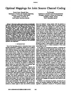
Binary sources with different memory structure. Parameters are chosen such that the entropy rate is 0.516 bit/symbol for each source.

bits. Notice that the optimal number of systematic bits depends on the source statistics and can be optimized. Alternatively, a doubly-asymmetric turbo code can be used, whereupon one component code satisfies the Recursive Self Quick-Look-In property [13]. Hence, applying the same puncturing pattern to both parity sequences of the QLI component code, the source symbol can be reconstructed for each non-erased parity bit pair. Notice that the number of perfectly known source bits depends on the puncturing rate and cannot be adjusted.

4

0.5

0.5

0.5

0.

I.I.D. source Fig. 3.

0.005

b s 2 un

9

4

0.2 5

0.0 5

28 0.

0.005

0.72

28 0.

0.72 0.1154

5 0.0

0.1

5 0.2

3

0.995

0.9

p(u)

0.8846

0.0

5

0.1

1

Numerical Results

4.1 Review of Entropy Calculation I.I.D. source - This memoryless source is characterized by its probability mass functionPp(u). The entropy rate is given by H∞ = H(U ) = − u p(u) log2 p(u). Markov source - This type of source is based on a stationary Markov process which is described by its initial state distribution π and state transition matrix A. There is a mapping from each state sn to one output symbol un in our notation.PThe entropy P rate of this source is H∞ = − sn p∞ (sn ) sn+1 asn sn+1 log2 asn sn+1 , whereas p∞ (sn ) is the stationary state distribution and is obtained by solving AT p∞ (sn ) = p∞ (sn ) w.r.t. P p∞ (sn ) = 1. HMM source - The upper P bound of the entropy rate is H(Un |U 1n−1 ) = − un p(un1 ) log2 p(un |u1n−1 ) 1 andP the lower bound is H(Un |U 1n−1 , S1 ) = − un ,s1 p(un1 , s1 ) log2 p(un |u1n−1 , s1 ). 1 The bounds can be calculated very efficiently by utilizing the HMM parameters as well as the forward/backward algorithm in its original description on perfect symbol knowledge. When determining the upper bound it is easy to see that the joint probability of the sequence un1 is obtained by X αn (sn ) . (9) p(un1 ) = sn

The conditional probability of un given the past can be expressed by X p(sn , u1n−1 ) , (10) p(un |u1n−1 ) = bs n u n p(u1n−1 ) sn whereas the numerator is given as X αn−1 (sn−1 )asn−1 sn . p(sn , u1n−1 ) =

(11)

sn−1

The denominator of (10) is computed similar to (9). In order to calculate the lower bound we use (9)-(11), but replace αn (sn ) by αn0 (sn ) = p(un1 , sn |s1 ) with initialization α10 (s1 ) = bs1 u1 . One drawback of calculating the bounds is the computational complexity, as it grows exponentially with the sequence length.

4.2 Sources of Reference The presented numerical results show source coding rates when compressing data of three different sources, which are illustrated in Fig. 3. The sources differ in their memory structure: one is memoryless, the second is based on a (visible) Markov process and the other is an HMM source. All of them output binary symbols (M = 2). The source parameters are chosen such that the entropy rate equals each other. Consequently the difficulty in compressing them lies in recognizing the memory type and in modeling the source parameters.

4.3 Parameter Setup We simulated 1000 blocks, each consisting of N = 16384 binary symbols. The turbo code was either a symmetric, non-systematic, rate one half code with polynomials (11/13) or an asymmetric, non-systematic, rate one third code with (15/13, 6/13, 13/15) . Both component codes were separated by an s-random interleaver in each case. Furthermore we also used an srandom interleaver in combination with puncturing as explained in Section 2.3. When compressing sources with memory, we doped every 6th source bit, whereas no source bits were sent for the i.i.d. source. Conventional source coding was performed by a Huffman code

as specified in [14]. Thereby eight consecutive bits of the source sequence are grouped to one symbol and the relative frequencies are computed to generate the Huffman tree.

4.4 Simulated Compression Rates As shown in Table II, simulation results clearly indicate that our proposed scheme outperforms Huffman coding, if the source parameters (A, B, π) are perfectly known and we dope systematically. The difference is bigger when compressing sources with memory. The simulated rate for the i.i.d. source complies with the results obtained with perfect SSI (compare to [15]). The compression rates are slightly inferior to systematic doping when applying the asymmetric turbo code. There might be several reasons: 1) The QLI component code does not match the other component code very well. This can be concluded by comparing the rates for the memoryless source when the SSI is perfectly known. 2) The systematic information is not distributed regularly on the HMM decoder input compared to doping. Therefore, this decoder will have difficulties to synchronize with the source sequence and estimate a proper state sequence. However if the component codes are synchronized to each other and the puncturing pattern is chosen such that the systematic bits are regularly allocated on the HMM decoder trellis, rates similar to or better than doping the source bits should be obtained. The estimation of the source parameters results in a degradation of the compression efficiency in the case of systematic doping, but Huffman coding is still outperformed when compressing sources with memory. The degradation is higher when using the asymmetric turbo code. Remember that the systematic doping rate is already adapted to the statistics of the source whereas the QLI code suffers because of the two reasons stated above.

5

Conclusions

The extension of lossless turbo source coding to compress sources with memory is considered. We serially concatenated a turbo code, which is used to restore the source sequence, with a source decoder based on TABLE II AVERAGE COMPRESSION RATES AND STANDARD DEVIATION source type entropy

Turbo Compression

Huffman Coding Perfect Source Model systematic doping Perfect Source Model Quick-Look-In Estimated Source Model systematic doping Estimated Source Model Quick-Look-In

µ ˆR σ ˆR µ ˆR σ ˆR µ ˆR σ ˆR µ ˆR σ ˆR µ ˆR σ ˆR

i.i.d. 0.516 0.643 0.009 0.621 0.011 0.802 0.012 0.706 0.033 0.799 0.013

Markov 0.516 0.679 0.009 0.604 0.012 0.661 0.014 0.618 0.013 0.678 0.014

HMM 0.516 0.686 0.009 0.604 0.012 0.664 0.015 0.623 0.014 0.750 0.092

a Hidden Markov Model. The purpose of the latter decoder is to model the source by estimating its parameters. One major problem of our scheme is the start-up of joint estimation-decoding. We showed that systematic doping and the usage of an asymmetric turbo code with QLI property improve the starting conditions. Furthermore an alternative puncturing algorithm called adaptive successive rate refinement was presented. The complexity of this algorithm is fixed and the number of analysis by synthesis cycles depends on the desired granularity. Simulation results indicate that turbo source coding outperforms Huffman coding when encoding sources with memory.

References [1] G. Caire, S. Shamai, and S. Verd´ u, “A new data compression algorithm for sources with memory based on error correcting codes,” in Proc. IEEE Information Theory Workshop, Paris, France, April 2003, pp. 291–295. [2] ——, “Universal data compression with LDPC codes,” in Proc. International Symposium on Turbo Codes & Related Topics, Brest, France, September 2003, pp. 55–58. [3] J. Garc´ ıa-Fr´ ıas and Y. Zhao, “Compression of binary memoryless sources using punctured turbo codes,” IEEE Communications Letters, vol. 6, no. 9, pp. 394–396, September 2002. [4] J. Hagenauer, J. Barros, and A. Schaefer, “Lossless turbo source coding with decremental redundancy,” in Proc. International ITG Conference on Source and Channel Coding, Erlangen, Germany, January 2004, pp. 333–339. [5] N. D¨utsch, “Code optimization for lossless turbo source coding,” in Proc. IST Mobile & Wireless Communications Summit, Dresden, Germany, June 2005, paper 197. [6] N. D¨utsch and J. Hagenauer, “Combined incremental and decremental redundancy in joint source-channel coding,” in Proc. International Symposium on Information Theory and its Applications, Parma, Italy, October 2004, pp. 775–779. [7] N. D¨utsch, H. Jenkac, T. Mayer, and J. Hagenauer, “Joint source-channel-fountain coding for asynchronous broadcast,” in Proc. IST Mobile & Wireless Communications Summit, Dresden, Germany, June 2005, paper 558. [8] J. Garc´ ıa-Fr´ ıas and J. D. Villasenor, “Turbo decoding of gilbert-elliot channels,” IEEE Transactions on Communications, vol. 50, no. 3, pp. 357–363, March 2002. [9] J. Garc´ ıa-Fr´ ıas and W. Zhong, “LDPC codes for compression of multi-terminal sources with hidden markov correlation,” IEEE Communications Letters, vol. 7, no. 3, pp. 115–117, March 2003. [10] J. Garc´ ıa-Fr´ ıas and J. D. Villasenor, “Joint turbo decoding and estimation of hidden markov sources,” IEEE Journal on Selected Areas in Communications, vol. 19, no. 9, pp. 1671– 1679, September 2001. [11] ——, “Combining hidden markov source models and parallel concatenated codes,” IEEE Communications Letters, vol. 1, no. 4, pp. 111–113, July 1997. [12] L. R. Rabiner, “A tutoial on hidden makov models and selected applications in speech recognition,” Proceedings of the IEEE, vol. 77, no. 2, pp. 257–286, February 1989. [13] P. Massey and D. Costello, “Turbo codes with recursive nonsystematic quick-look-in constituent codes,” in Proc. International Symposium on Informatino Theory, Washington, DC, June 2001, p. 141. [14] M. Nelson, The Data Compression Book. Prentice Hall, 1991, ch. 3, The Dawn Age: Minimum Redundancy Coding, pp. 29– 80. [15] J. Hagenauer, N. D¨utsch, J. Barros, and A. Schaefer, “Incremental and decremental redundancy in turbo source-channel coding,” in Proc. International Symposium on Control, Communications and Signal Processing, Hammamet, Tunisia, March 2004, pp. 595–598.