T-ITS-07-04-0062
1
Space-Based Passing Time Estimation on a Freeway Using Cell Phones as Traffic Probes Keemin Sohn and Keeyeon Hwang
Abstract—This study examines the usability of mobile cellular networks to obtain traffic information on a freeway. The question of whether a mobile station (cell phone) can play an acceptable role as a probe for collecting traffic information on a freeway is examined. A space-based approach, wherein the probe vehicles transmit information to roadside devices as they pass through reference points, is exploited rather than a time-based approach, wherein the probe vehicles report information for every specific instant of time. The latter has been of concern to most researchers interested in the use of a mobile cellular network for collecting traffic data. First, a simple analytical model is introduced to address the usability of cell phones as traffic probes and to pinpoint which factors affect the qualification of probe phones when the space-based approach is adopted. Second, simulation experiments are also employed to deal with more realistic traffic conditions as supplementary tools for the analytical model. Finally, the actual traffic data on a freeway was considered to validate the above two hypothesized traffic conditions. The findings show that there are three main factors that affect the qualification of cell phones as a traffic probe: first, the speed profile of the probe phone in cell coverage; second, the variability of handoff location where the probe phone switches its jurisdictional cell; and lastly the locational relationship between a reference point and a speed jump (or drop) point in cell coverage. Index Terms— Cellular communication System, Freeway, Passing time , Traffic Probe,
I. INTRODUCTION
T
raffic information from probe vehicles has great potential in improving the estimation accuracy of traffic situations, especially in locations where no traffic detector is installed. Reference [1] described how to use vehicles as probes in detail by combining information scattered among many different engineering fields. Reference [2] also suggested three possible approaches by which probe vehicles can transmit information, based on the background of [1]. The first approach is space-based, in which probe vehicles transmit information to roadside devices as they pass observation points. This type of approach is often referred to as automatic vehicle identification
Keemin Sohn is with Metropolitan Planning Research Group, Seoul Development Institute, 391 Seocho-dong Seocho-gu Seoul Korea 137-071 (corresponding author; phone: +82-2149-1110; fax: +82-2149-1120; e-mail: kmsohn@ sdi.re.kr). Keeyen Hwang is with the Department of Urban Engineering, Hongik University, 72-1 Sangsu-dong Mapo-gu Seoul Korea 121-791 (e-mail:
[email protected]).
(AVI). Traffic data could be obtained by means of various AVI technologies, such as a beacon-based system, an electronic toll tag system, and an automatic license-plate-recognition system. The second approach is time-based, in which probe data are reported at every specific instant of time, regardless of the position of the probe vehicle, and the data can be obtained from the GPS-based system or a beacon-based system. The last approach is event-based, in which traffic information is reported when a particular event occurs, for example, traffic accident reports from drivers through cellular phones. Some researchers have recently become interested in the possibility of using cell phones as traffic probes [3], [4]. Most of them only adopted the time-based approach to collect traffic information from the cell phones and cellular mobile networks. Reference [3] introduced several techniques for tracking the position of cell phones in a mobile cellular network, namely, the signal profiling technique, the angle-of-arrival technique, and the timing measurement technique. It is impossible to rule out location errors entailed in location data obtained by the time-based approach using the cell phones. The imperfect locations should then be subjected to a map-matching process to derive useful traffic information from them. This study focuses on the issue of whether cell phones could play an acceptable role as space-based traffic probes to collect traffic information on a freeway. It is not appropriate to assert that cell phone probing is superior to other existing space-based methodologies (e.g., AVI), which have an exact detection location that is determined only for the purpose of traffic surveillance. However, it is worth examining the loss in accuracy and efficiency when the cell phone probing substitutes for the existing AVIs, because the space-based cell phone probing has a great potential for traffic surveillance in spite of the drawback. The term “space-based” in cell phone probing signifies that a cell boundary is regarded as a point detector. The space-based approach makes it possible to save the battery consumption of the probe phones and to relieve the additional system load on mobile cellular networks because a probe phone does not require the location to be updated frequently. A location update is needed when the probe phones enter and leave only a cell, the coverage of which includes observation points on a freeway. The passing time at an observation point on a freeway can then be estimated from both the entry and exit times at boundaries of a cell that include the point. Even though this approximation also entails a location error, the space-based approach deserves to be examined, based on the fact that this approach, along with mobile cellular technologies, has a great potential in the traffic surveillance system, compared with the
T-ITS-07-04-0062 existing AVI technology. It makes the best use of the already installed infrastructure of mobile cellular networks, thus giving rise to great cost savings in the establishment and maintenance. The spatial coverage of traffic surveillance is maximized because almost the entire area is covered by mobile cellular networks. It is very advantageous in the market penetration, since it already has a huge user base. A situation where a probe phone is missed while being tracked is unlikely to happen, since missing a phone means a failure in communication services, which matters when considering the quality of communication services. Such benefits led us to investigate the performance of the space-based cell probing in spite of the limitation on its accuracy. This study begins with the question of whether a cell phone could play an acceptable role as a probe, and thus examines the effect of several factors on the qualification of a cell phone acting as a traffic probe, when the space-based approach is adopted along with mobile cellular technologies. The present investigation involved both analytical and empirical approaches. A simple analytical model was developed to account for the usability of cell phones as probes and the simulation experiments were also employed to deal with the more realistic traffic conditions together with the analytical model. Lastly, the accuracy and efficiency of the estimated passing times at an observation point was examined by using actual speed profiles obtained from consecutive aerial photos on a freeway segment during a one-hour period.
II. CELL POSITIONING OVERVIEW Conventional mobile communication service consists of two operations, location-updating and paging. A brief description of the two operations has been given by [5]. The network coverage area is partitioned into a number of location areas (LAs). Each LA consists of a group of cells, each of which is served by a base station (BS). The BSs of an LA periodically broadcast an identifier associated with that area. When active cell phones enter a new cell, they compare the identifier stored with the broadcast identifier of the LA. If the two identifiers differ, the cell phone recognizes that it has entered a new LA and a location update is performed. As an incoming call arrives, the network locates the called cell phone by paging all cells within an LA. Therefore, the current location of a cell phone is only identified by the LA in a conventional cellular operation. Each moving active cell phone in a mobile cellular network performs an idle handoff operation when it switches its jurisdictional BS. Reference [6] described the types of handoff in detail. The handoff can be classified into two types, on-call and idle handoff, according to its function. The on-call handoff, which is generally called handoff, makes it possible to maintain incessant call, when a phone in use is moving across multiple cells. On the other hand, the purpose of idle handoff is to maintain operation channels to at least one BS, when a cell phone is on but not in use. The idle handoff is of major concern in traffic surveillance of this study. Handoff is also divided into two broad categories according to the physical method for processing hard and soft handoffs. They are characterized by “break before make” and “make before break.” In the hard
2 handoff, current channels are released before the new channels are used. In the soft handoff, both the existing and new channels operate concurrently during the handoff process. The terms “hard handoff” and “idle handoff” are used interchangeably in this investigation because the idle handoff generally adopts the hard handoff type. If a cell phone were to function as a traffic probe, its location information should be reported when it enters and leaves the reference cells, in the coverage of which observation points on a freeway reside. However, just the idle handoff occurs in a cell phone, without the location update [6]. An additional system is required to inform a mobile switching center (MSC) of the idle handoff and then the reported information is processed further. This system revision is not required for every phone and cell, but is necessary only for probe phones and reference cells. The staff in charge of the network management in a company providing mobile communication services concluded that such a system revision is not technically difficult. In the case of decision of the investment for that revision, however, it matters most to have a consensus between the party adopting phone probes and the company possessing mobile cellular networks. The traffic surveillance, based on handoffs, has been studied by several researchers [7], [8], [9], [10]. They proposed a methodology for estimating the traffic parameters, such as density, volume, and speed in segments divided by cell boundaries. Since the researchers focused on the estimation of aggregate traffic parameters, they overlooked the potential of individual cell phone as a traffic probe. Tracking cell phones as traffic probes can provide the foundation for estimating travel times and the origin–destination flows, both of which are most important in the intelligent transportation system (ITS). Reference [11] has described the application of proposed cell probing method for the estimation of origin–destination flows. Moreover, in all earlier works except for [11], the traffic parameters are computed with respect to each road segment, divided by cell boundaries. It is necessary to determine the initial state of traffic parameters on the boundaries. The estimation result obtained from the model is also summarized for the segment. However, the handoff locations are not determined by the transportation network but by the mobile cellular network. The handoff location determined by the mobile cellular network has no facilities to detect the traffic state and has little meaning in the transportation aspect. There has been no other study that clarifies the relationship between the traffic state on cell boundaries and the transportation reference point. Our work also deals with the variability of handoff location, which has been ignored in the earlier studies, although it is confined to the estimation of passing times. Reference [12] gave a detailed description of the ignition of idle handoff (hard handoff). If the signal strength from the current jurisdictional BS is less than a threshold value, then another BS with the strongest signal is selected as a new jurisdictional BS. The newly selected signal, of course, should be stronger than the threshold (Fig. 1).
T-ITS-07-04-0062
3 Signal strength
Signal strength
Signal strength of new base station Threshold value Probe Vehicle
Current base station
Handoff location
New base station
Fig. 1. Ignition of Idle handoff
It is very important to locate where the idle handoff takes place and determine how the location varies in utilizing a cell phone as a traffic probe. The strength of the signal emitted from a BS is not deterministic, but may vary according to both the internal fluctuations of the radio wave itself and the external environment, such as weather conditions, the amount of communication traffic, and the condition of facilities or buildings around the cell boundary area. It should be noted that there has been no test on the variation in idle handoff locations. In fact, conducting such a field survey would be complex because the cellular network is owned by private companies and the network configuration is protected as an operational secret. In this study, the locations are assumed to vary stochastically so that a normal distribution can be adopted. Evidently, no matter what kind of stochastic distributions are employed, it would be acceptable, so long as they are calibrated from field data. A mobile cellular network covers all the areas where its communication service is available, which implies that the freeway to be monitored is also covered with a series of cells. Especially in the case of a freeway in rural areas, the mobile cellular network is provided with a group of cells exclusively for the freeway, the shape of which is narrower and longer than that of the conventional cells in urban areas. The newly proposed cell-based methodology involves all possible reference points residing on the freeway. For example, the location of existing detectors or variable message signs (VMS), the entry and exit points of the freeway, and other points, based on which travel times are calculated.
III. PASSING TIME ESTIMATION USING CELL PHONES AS PROBES This study focuses on the accuracy and efficiency of the estimated passing time when using cell phones as traffic probes. The term “passing time” indicates the time when a probe actually passes a reference point in the transportation network. To prevent obscurities and confusions in the paper, the terms “passing time” and “crossing time” are defined differently. The passing time is used at a reference point in the transportation network, whereas the crossing time (handoff time) is used at cell boundaries in the mobile cellular network.
A. Passing Time Estimation at Reference Points The passing time of a moving probe phone at a reference point can be estimated to be a convex linear combination of crossing times at both the boundaries of the reference cell. (1) t est (a ) = (1 - a )t (0) + at (1) a denotes the fraction of the distance between a reference point and the deterministic entering cell boundary (all figures in this paper are depicted such that the probe moves from left to right). t (0) and t (1) represent the crossing times at the entry and exit cell boundaries, respectively. t est (a ) is the estimated passing time for a reference point. There would be no erroneous estimation under the ideal condition. The ideal condition can
be defined as a condition where the speed of the probe phone is unchanged in a cell and the handoff always occurs at consistent locations. If a reference cell size were asymptotically small or a reference point exactly matches the deterministic cell boundary, then the cell phone probe system would also be identical to the existing space-based AVI system, irrespective of the speed profile of the probe phone. In contrast to the above-described cases, passing time estimates would be biased and inefficient when applied to the real world. In the following sections, the efficiency and accuracy of the estimation in the case where the cell boundaries are stochastic and the speed profile of probe phones varies is examined. The locational relationship between the reference point and the reference cell boundaries may give rise to a time-lag problem in real-time applications, even under the ideal condition, because the passing time is not calculated until the probe phone leaves the exit boundary of the reference cell. However, it would never raise any complications in offline applications. This problem is not dealt with here, because the major concern in the present investigation is only the spatial issue regarding cell phone probes. B. Simple Model A simple model was established to describe the two deviations from the ideal condition. The first deviation is a change in the probe phone’s speed profile. The speed profile of the probe phone along the freeway in the reference cell is expressed by (2). (2) V ( X ) = V0 e b X where V ( X ) denotes the speed of the probe phone at location X , V0 and VD are the probe speeds at the entry and exit cell boundary, respectively, and b is a parameter indicating the rate of speed change. b can be replaced by (ln V0 - ln VD )
D
to take
into account the effect of speed differences between the entry and exit cell boundaries, where D is the distance between the average entry and exit cell boundaries. It is a discretionary assumption that the speed of the probe phone varies monotonically along the freeway. However, the present simple model is sufficient to account for the relative effect of the speed difference between the two boundaries of the reference cell on
T-ITS-07-04-0062
4
the accuracy and efficiency of a probe phone’s passing time estimates at the reference point. In the next section another speed profile, which can address the abrupt speed change, will be taken into account along with simulation experiments. Later in this study, the two types of speed profiles will be verified in the real-world traffic condition. Cell boundary fluctuation is the second deviation from ideal conditions. As seen in Fig. 2, it is assumed that the cell boundaries vary stochastically. X 0 and X D are the only
random variables in the model and denote the actual handoff locations near the entry and exit cell boundary, respectively. They are assumed to follow a normal distribution, as given in (3), where s0 and s D are the standard deviations of the distribution (the subscript is analogous to those in X 0 and X D ).
X 0 ~ N (0, s 02 ) , X D ~ N ( D, s D2 )
(3)
V (1 - a ) D
aD X 0 ~ N (0, s 02 )
X D ~ N ( D, s D2 )
Reference Point
b >0
V ( X ) = V0 e b X
b =0 V0
b 0
VD X
0
LD
D
(b) Fig. 2. Speed profile model: (a) exponential speed change; (b) abrupt speed change
T-ITS-07-04-0062
5
t ( X ) represents the passing time at location X and can be
derived by integrating the inverse of V ( X ) along the freeway from zero to X , when the average entry cell boundary is set to zero. X dw 1 (4) t( X ) = ò = (1 - e - bX ) , if b ¹ 0 0 V (w ) V0 b t est (a ) is the passing time estimator at a reference point ( aD ) and can be calculated to be the linear combination of t ( X D ) and t ( X 0 ) . a is the fraction of the distance from a reference point and the average entry cell boundary.
1 (5) 1 - ae - bX D + (1 - a )e - bX 0 V0 b The mean and variance for the passing time estimate at a reference point can be derived easily by using the well-known relationship between the parameters of normal and log-normal distributions. The assumption that the speed of a probe varies
[ {
}]
[
Std .Dev. = Var t est (a )
(sec)
100
]
[
2 2 2 2 1 1 - (ae - bD +0.5 b sD + (1 - a )e 0.5 b s0 ) V0 b 2 2 2 2 1 Var t est (a ) = a 2 e -2 bD + b sD (e b sD - 1) + 2 (V0 b )
[
]
E t est (a ) =
[
]
(6)
[
]
2 2
]
2 2
(7) (1 - a ) 2 e b s0 (e b s0 - 1) It is also crucial to identify the difference between true and mean passing times, because it is impossible to rule out a bias in the estimation. The bias of the estimate can be calculated by using (8). Bias t est (a ) = E t est (a ) - t (aD) 2 2 2 2 1 -abD (8) = e - (ae - bD + 0.5 b sD + (1 - a )e 0.5 b s0 ) V0 b The effect of two deviations on variance and bias is well described in Fig. 3(a), (b). It is shown in Fig. 3(a), (b) that the speed difference ( V0 - VD ) and cell boundary variation ( s ) have a strong influence on both efficiency and accuracy, respectively.
[
t est (a ) = at ( X D ) + (1 - a )t ( X 0 ) =
exponentially along the freeway segment makes it possible to express both the mean and variance in closed form.
] [
]
[
]
(sec)
Bias = E[t est (a )] - t (aD)
100
90
90
80
80
70
70
60
60
50
50
40
40
30
30
20
20 10
10 0 10
20
s = 100
30
s = 150
40
0
V0 - VD (km / h) 50
s = 200
60
70
s = 300
s = 250
10
80
s = 350
20
s = 100
30
40
s = 150
[
6.5 6.0 5.5 5.0 4.5 4.0 3.5 3.0 2.5 2.0
50
s = 200
(a) Std .Dev. = Var t est (a )
(sec)
V0 - VD (km / h)
60
70
s = 300
s = 250
80
s = 350
(b)
]
Bias = E[t est (a )] - t (aD)
(sec) 2
2 1 1 0 -1
0
0.1
0.2
0.3
0.4
0.5
0.6
0.7
0.8
0.9
1
-1 -2 -2
0
0.1
0.2
0.3
0.4
0.5
0.6
0.7
0.8
0.9
a
1
a b 0
b =0
b 0
b =0
(d)
Fig. 3. Results from simple model: effect of speed difference and cell boundary variation (a) on variance; (b) on bias ( D is set as 500 m, V0 as 100 km/h, a as 0.5, and the variances of both the entry and exit cell boundaries are assumed to be identical [ s
= s 0 = s D ]); effect of reference point
location; (c) on variance; (d) on bias ( D is set as 500 m, the variances of both the entry and exit cell boundaries are assumed to be identical [s
= s 0 = s D ] and set as 100 m. The negative [positive] b
km/h [100 km/h]).
is designated as -0.001 [0.001], such that V0 is 100 km/h [60.7 km/h] and VD is 60.7
T-ITS-07-04-0062
6
If one of the two variables decreases, then the variance and the bias are not largely affected by the other. In particular, when the speed difference is small, the effect of boundary variation on variance and bias is trivial and vice versa. It is fortunate that the possibility of the worst situation, in which both the variables are large, seems to be relatively low. The partial derivatives of variance and bias with respect to a are derived, by which the effect of locational relationship between a reference point and the cell boundary can be identified.
[
]
2 2 2 2 ¶Var t est (a ) 2 = (e - 2 b D + 2 b s D - e - 2 b D + b s D 2 ¶a (V0 b )
[
2 2
2 2
2 2
+ e 2 b s0 - e b s0 )a - (e 2 b s0 - e b ¶Bias[t est (a )] 1 = (e 0.5 b s - e - bD +0.5 b s ) ¶a V0 b - b De -abD ]
[
2 2 0
2 2 s0
)
]
(9)
2 2 D
(10) Equation (11) indicates the fraction value of the minimum variance point ( a * ). If the variances of both the boundaries are equal ( s
[
= s 0 = s D ), then Equation (11) reduces to (12).
]
est
¶Var t (a ) =0 , ¶a
e 2b
a* =
2 2
2 2 s0
- eb
e - 2 bD + 2 b s D - e - 2 bD + b a * = 1 - 2 bD (e + 1)
2 2 sD
2 2 s0
+ e 2b
2 2 s0
- eb
2 2 s0
(11) (12)
Equation (13) indicates the fraction value of the maximum bias *
point ( a ). It implies that the maximum bias point resides between both the cell boundaries, unless the probe’s speed is drastically increased or decreased. bD æ ö lnç 0.5 b 2 s 2 ÷ - bD + 0.5 b 2 s D2 ¶Bias t est (a ) 0 * -e ø (13) = 0, a = èe bD ¶a Fig. 3(c), (d) depicts the effect of the locational variation in the reference point on variance and bias. The estimation is bias-free and the minimum variance point is at the exact middle, between the average entry and exit boundaries, when the probe speed is stable ( b asymptotically approaches zero). This is also consistent with the implications in (12). The minimum variance point approaches the entry (or exit) cell boundary when the probe speed decreases ( b < 0 ) (or increases [ b > 0 ]) along the freeway. It is interesting to note that the variance at a point near the middle of the cell is smaller than those near either of the cell-boundary areas. This indicates that an estimate at a point near a cell boundary, where direct detection occurs, is less efficient than an estimate made at other locations. The bias leads to an underestimation in passing time, when the probe speed decreases and vice versa. As seen in Fig. 3(c), (d), the maximum variance point resides in the cell boundary areas and the maximum bias point is located near the middle of the cell. This implies that a large variance point never coincides
[
]
with a large bias point. Thus, it is fortunate that a large variance (bias) is compensated by a small bias (variance). The effect of the overall speed of the probe phone, which might reflect the flow state on the freeway, on the efficiency of the estimation was examined. Equation (14) indicates the partial derivative of variance with respect to the probe-phone initial speed when the probe’s speed is constant along the freeway ( b = 0 or V0 = VD ). According to (14), the variance in the estimation decreases dramatically (at the second-power rate of the initial speed) with the increasing speed of the probe phone. The more stable and the higher the speed of the probe phone, the more efficient the proposed estimation would be.
[
]
¶Var t est (a ) - (as D2 + (1 - a ) s02 ) = ¶V0 V02
(14)
C. Simulation Experiments The simple model does not take into account the various speed profiles of a probe phone. This section deals with a more plausible speed profile. However, a more realistic speed profile prevents the variance and bias of the estimation from being derived in the closed form. The simulation experiment is only a tool for evaluating the accuracy and efficiency of passing time estimates. It is well known that vehicle speed on a freeway is apt to drop abruptly when the vehicle encounters the queue propagated from an upstream bottleneck. The recovery of speed also occurs abruptly as the vehicle passes through the bottleneck area. A new speed profile function, which can be used to approximate the drastic speed jumps or drops, is introduced as follows; the notations used here are identical to those used in the simple model. Only two differences are found in b and L . Unlike the simple model, b , representing how drastically the speed changes, is determined independent of V0 and VD . The larger the b , the more abrupt the speed change is. L is the fraction of the speed changing location. V0 - VD (15) V (X ) = + VD , b > 0 1 + e b ( X - LD ) Fig. 2(b) shows a typical situation where the probe vehicle may go through a speed drop in a freeway. t ( X ) can be calculated by integrating the inverse of V ( X ) along the freeway from zero to X . Equation (18) is easily derived by simple algebra, including integration by substitution. X dw X æ V0 - VD ö æ V0 e - b ( X - L ) + VD ö (16) ÷ ÷ lnç t( X ) = ò = +ç 0 V (w ) VD çè VDV0 b ÷ø çè V0 e bL + VD ÷ø Passing time is estimated in the same manner as adopted in the simple model case. The two random variables, X 0 and X D , are the source of the stochastic variability of the estimation. Two independent normal variates generate X 0 and X D , based on (3), and an estimate of t est (a ) is then obtained from them. This process is repeated until a sufficient sample size (10,000 in this investigation) is reached. The process results in the mean, variance, and bias of the estimate. The effect of two factors, such as the variation of cell boundaries
T-ITS-07-04-0062
7
and the speed difference between entry and exit boundaries, was tested and compared with the results from the simple model. Fig. 4(a), (b) depicts the effect of the two factors on the variance and bias of the passing time estimation in the case of a speed drop. The b value of 0.6 is selected such that the speed drop at the middle of the reference cell is abrupt. All the findings of the simulation experiments were similar to those of the simple model. The realistic speed profile of the probe-phone resulted in a more efficient and accurate estimation in terms of the variance and the bias. Especially, the variance and bias are much smaller than those of the simple model. This finding suggests that the gradual change in the probe-phone speed deteriorates the accuracy and efficiency of the passing time estimation to a greater extent than an abrupt change. There might also be local fluctuations of probe-phone speed, the amplitude of which is relatively small. A new speed profile was created by introducing a fluctuation in the speed profile. The variation is derived from the log-normal distribution, the mean of which is assumed to be a constant speed profile. The variance in the distribution ( s 2 ) and the periodic length of
fluctuation (fluctuation cycle length) are varied by monitoring the accuracy and efficiency. The newly created speed profile is considered to be deterministic, once generated. The numerical integration is adopted to derive the passing time function ( t ( X ) ), which entails additional errors and computational burdens. It is assumed that every condition is identical to the case of an abrupt speed change, except that there is no speed difference between both cell boundaries ( V0 = VD ) and that the standard deviation of the cell boundary is set to 100 m ( s = s0 = s D = 100 m). As a result, the fluctuation cycle length hardly affects the estimated passing time, unless the standard deviation of the log-normal distribution ( s L ), which represents local fluctuations in the probe-phone speed, is sufficiently large. Fig. 4(c) shows that s L has little effect on the variance and bias of the passing time estimation when the speed of the probe phone is high. However, in Fig. 3(d), it can be seen that the local fluctuations in speed can give rise to a deterioration of the accuracy and efficiency of the estimation when the speed level is low.
L
[
(sec)
Std .Dev. = Var t est (a )
100
]
Bias = E[t est (a )] - t (aD)
(sec)
100
90
90
80
80
70
70
60
60
50
50
40
40
30
30
20
20
10
10
0 10
20
s = 100
30
s = 150
40
V0 - VD (km / h) 50
s = 200
0
60
s = 250
70
s = 300
80
10
s = 350
20
s = 100
30
40
s = 150
[
Std .Dev. = Var t (a )
]
50
60
s = 250
s = 200
(a) est
V0 - VD (km / h)
70
80
s = 300
s = 350
(b)
[
Bias = E[t est (a )] - t (aD)
Std .Dev. = Var t est (a )
(sec)
(sec)
]
Bias = E[t est (a )] - t (aD)
100
100
90
90
80
80 70
70
60
60
50
50
40
40
30
30
20
20
10
10 0
0 5
10
15
20
25
30
35
40
45
50
55
5
10
15
20
25
30
35
40
45
50
55
sL
sL (c)
(d)
Fig. 4. Results from simulation experiments: effect of speed difference and cell boundary variation: (a) on variance; (b) on bias (all conditions are the same as the simple model, except that L is set to 0.5 and b to 0.6); effect of local fluctuation in probe phone speed: (c) high speed ( V0 = VD = 100 km/h); (d) low speed ( V0 = VD = 30 km/h).
T-ITS-07-04-0062
[
Std .Dev. = Var t est (a )
8
]
point resides in the middle area between the cell boundaries, when the speed-jump point is near the cell boundary. On the other hand, it approaches the exit cell boundary as the speed-jump point approaches the middle area between the cell boundaries. Identifying the variance at points where two locational variables are equal would be worthwhile, because speed jumps and drops frequently occur near the merging and diverging areas and the merging and diverging points are ideal reference points for calculating travel time on a freeway. Line BB′ connecting such points indicates that the minimum variance point is inclined somewhat towards the exit cell boundary ( a = L = 0.7). The minimum variance increases as the speed jump location approaches the exit cell boundary. This finding confirms that the longer the distance of high speed, the more efficient is the estimation. The two axes are rotated in Fig. 5(b) such that the variance surface could be presented more clearly. The variance surface in the case of a speed drop is symmetric to that in the speed jump case. Line AA′ in Fig. 5(b) shows that the minimum variance point resides in the middle, between both cell boundaries, when the speed-drop point is near both cell boundaries and that it approaches the entry cell boundary as the speed-drop point approaches the middle area between the cell boundaries. Line BB′ indicates that the minimum variance point is inclined somewhat to the entry cell boundary ( a = L = 0.3). The bias in the estimation is depicted in Fig. 5(c). The passing times are overestimated in the case of a speed drop and vice versa. The maximum bias occurs when both the reference point and speed-change point reside near the middle area between the cell boundaries. The bias and the variance along the line that connects points where two locational variables coincide with each other ( a = L ) are symmetrical with respect to each other. Thus, there is no point where both variance and bias are maximized simultaneously.
8.0
7.0
6.0
B’
A’
B 5.0
4.0
3.0
L
1.0 0.5
A
-0.1 0.1
0.5
1.0
a
(a)
[
Std .Dev. = Var t est (a )
]
8.0
7.0
6.0
A
B’
B 5.0
a
4.0 1.0 0.5 3.0 0.1 -0.1 0.1 0.5
A’ 1.0
L
(b)
[
Bias = t (aD) - E t est (a )
]
5.0
4.0
D. Evaluation of Passing Rime Estimates
3.0
V0 > VD 2.0
L
a -2.0
V0 < VD
-3.0
-4.0
-5.0
(c) Fig. 5. Effect of locational variables: (a) variance in case of speed jump ( V 0 < V D ); (b) variance in case of speed drop ( V > V ); (c) bias in both cases. 0 D
The effect of the locational relationship between the reference point ( a ) and the location of a speed jump or drop ( L ) on passing time estimation was examined. Fig. 5 shows the variance and bias as a function of a and L . Fig. 5(a), (b) represents a speed jump and drop, respectively. In the case of Fig. 5(a), the minimum variance point varies with each speed-jump point. As can be seen from line AA′, the minimum
The passing time estimates in this investigation were evaluated from the data on actual speed profiles. These data were obtained from consecutive aerial photos of I-405 southbound at Santa Monica Blvd. in Los Angeles, California. The photos were taken at one second intervals for an hour. Fig. 6(a) depicts an aerial view of the freeway segment and the hypothesized cellular configuration. The maximum cell length was set to 400 m because the available length of the freeway segment is, at most, 492.5 m. The standard deviations in both the cell boundaries are assumed to be 100 m. A vehicle’s speed out of the freeway segment is assumed to be identical to the speed at which the vehicle enters or leaves it, so that the problem in which the simulated cell boundaries exceed the available range of the segment can be sorted out. Fig. 6(b) shows a sample of the actual speed profiles for vehicles on the freeway segment. The sample profiles can be roughly categorized into three groups, based on their varying patterns. Group A represents profiles of vehicles at the early stage of non-congested traffic, wherein most vehicles are able to travel at high speed. As the traffic on the entry ramp
T-ITS-07-04-0062
9
increases, the profiles for declining pattern that are included in Group B appear. Some profiles in Group B can be successfully fit into the simple exponentially decaying function (2), while others, involving an abrupt speed drop, might be modeled by a more realistic function such as (15). The profiles for Group C do not emerge until upstream congestion is propagated, even
back to the front of the freeway segment. It can be shown that the speed increases slightly as the vehicle passes the merging area in Group C profiles. Group C profiles can also be modeled by the simple function.
Speed(km/h)
400.0 m
A
B
262.4m
230.1m
C
492.5 m
Location(m)
(a)
(b)
Fig. 6. Data from aerial photos: (a) aerial view of I-405 southbound at Santa Monica Blvd; (b) speed profiles of actual vehicles.
[
Std .Dev. = Var t est (a )
(sec) 18
]
Bias = E[t est (a )] - t (aD)
(sec)
6
16
4
14
2
12 10
0 100m
8
150m
200m
250m
300m
350m
400m
-2
6
-4
4 2
-6
0 100m
150m
200m
250m
300m
Reference point
Group A
350m
400m
-8 Reference point ( X )
(X )
Group B
Group C
Group A
(a)
[
Std .Dev. = Var t est (a )
(sec)
Group B
Group C
(b)
]
Bias = E[t est (a )] - t (aD)
(sec)
12
4 3
10
2
8
1
6
-1
0 1oom
200m
300m
400m
-2
4
-3 -4
2
-5 -6
0 1oom
200m
Group A
D Group B
300m
400m
-7
D Group C
Group A
Group B
Group C
(c) (d) Fig. 7. Results from actual speed profiles: effect of the location of the reference point (a) on variance; (b) on bias; effect of cell length (c) on variance; (d) on bias.
Several sample profiles were selected for each group to evaluate the variance and bias for the passing time estimates. The averaged variance and bias across each speed profile is presented in Fig. 7(a), (b). This confirms the validity of our earlier findings. For each speed varying pattern (Groups A, B, and C), the locations of minimum variance and maximum bias in Fig. 7(a), (b) are very similar to those in the simple model
(Fig. 3(c), (d)). Again, the findings show that the variance and bias for passing times become larger with overall slower speed. One aspect omitted in the earlier sections is considering the cell length in the model. The effect of cell length on the variance and bias of the passing time estimation can be identified by using actual speed profiles. Fig. 7(c), (d) shows the variance and bias at the exact middle point of the freeway segment when the length of the reference cell involving the
T-ITS-07-04-0062
10
point ( D ) varies from 100 to 400 m. It is interesting that the passing time variance is stable, irrespective of the cell length, except for Group C. In particular, the cell length has no effect on the efficiency of the estimation unless the traffic is congested. On the other hand, the bias grows larger as the cell length gets longer in the case of Groups B and C, where the vehicle speed is not stable. This suggests that the bias is generated mainly from the speed difference between both cell boundaries and that the variance arises mainly from the cell boundary variation unless the overall speed is too low.
IV. DISCUSSIONS The space-based use of cell phones as traffic probes was investigated in detail. Several factors affecting the estimation of a cell phone passing time were identified. Speed difference between both boundaries of a reference cell had a substantial effect on the passing time variance and bias. The cell boundary variation was the other determinant of efficiency and accuracy of the estimation. A synergism existed between the two factors. The effect of the relationship between the locational variables on the estimation was identified, so that the location of the reference point could be designed in conjunction with a mobile cellular network in a more efficient and accurate manner, if it were possible to change their configurations for the purpose of traffic probing. The interaction between overall speed levels and local fluctuation of the probe speed was also investigated. The variance and bias of the estimation were affected by local speed fluctuations only when the overall speed was low. Concerning the actual speed profiles, most of the findings were consistent with those from the simple model. It is obvious that using cell phones as probes is the most promising where the traffic speed is high and stable. A cell phone probing system might not be a good supplement to the existing surveillance system. However, the system could enhance the quality of traffic information if it is integrated together with the existing surveillance systems. In particular, the system could collect traffic information from places where no other traffic detection facilities are present. There are several issues that should be addressed in further studies. This investigation focused only on determining whether cell phones can act as traffic probes. It would be necessary to delve into a study of collecting traffic information, such as traffic volumes, travel speeds, and travel times. Moreover, enhancing location accuracy should be of main concern in future researches. The proposed detection approach has a good prospect, because new technologies based on mobile cellular networks, such as wireless LAN (local area network) and WiBro (Wireless broadband), will prevail in the future. Such technologies have a much smaller cell dimension. Thus, their applicability for traffic surveillance will be superior to the proposed cell phone probing system. In particular, WiBro has a great potential for the traffic surveillance, which provides high speed wireless Internet service that is available anytime, anywhere, using portable terminal in stationary or in mobile environment. It is being developed and will be commercialized soon by the Korean telecom industry.
REFERENCES Y. Zhao, Vehicle Location and Navigation Systems, Norwood, MA: Artech House, 1997. [2] C. Nanthawichit, T. Nakatsuji and H. Suzuki, “Application of probe-vehicle data for real-time traffic-state estimation and short-term travel-time prediction on a freeway,” Transportation Research Record 1855, 2003, pp 49-59 [3] J.L. Ygnace, C. Drane, Y.B. Yim, R. de Lacvivier, “Travel time estimation on the San Francisco bay area network using cellular phones as probes,” California PATH Working Paper UCB-ITS-PWP-2000-18, University of California, Berkeley [4] C. Drane and J.L. Ygnace, “Cellular telecommunication and transportation convergence,” 4th International IEEE Conference on Intelligent Transportation Issues, 2001, Oakland(CA), USA [5] Z. Mao, C. Douligeris, “A location-based mobility tracking scheme for PCS networks,” Computer Communications 23, 2000, pp 1729-1739 [6] S.I. Bang, Digital mobile communication, Minjungkak, 2004 (in Korean) [7] R. Bolla , F. Davoli and A. Giordano, “Estimating road traffic parameters from mobile communications”, Proceedings of 7th World Congress on Intelligent Transportation System, Torino (ITS 2000, Italy). [8] R. Bolla and F. Davoli, “Road traffic estimation from location tracking data in the mobile cellular network”, Proceedings of Wireless Communications and Networking Conference 2000 IEEE, Vol. 3, pp. 1107–1112. [9] P.Z. Cheng, Z. Qiu and B. Ran, “Traffic estimation based on particle filtering with stochastic state reconstruction using mobile network data”, CD-ROM of Transportation Research Board 85th Annual Meeting, 2006. [10] V. Astarita, R. Bertini, S. D'Elia and G. Guido, “Motorway traffic parameter estimation from mobile phone counts”, European Journal of Operational Research, 2006, Vol. 175, no. 3, pp. 1435–1446. [11] K. Sohn and D. Kim, “Dynamic origin-destination flow estimation using cellular communication system”, in press, IEEE Transactions on Vehicular Technology, DOI: 10.1109/TVT.2007.912336 [12] Q.A. Zeng and D.P. Agrawal, Handoff in wireless mobile networks in handbook of wireless networks and mobile computing, John Wiley & Sons, 2002, ch. 1. [1]
Keemin Sohn was born in Seoul, Korea in 1968 and was educated at the Department of Civil Engineering, Seoul National University (SNU) and earned Ph.D in transportation planning at SNU in 2003. He is now working as a research fellow in Metropolitan Planning Research Group, Seoul Development Institute. Keeyenn Hwang was born in Seoul, Korea in 1958 and had a bachelor's degree in Social Science from Yonsei University. He received his Ph.D in Urban Panning from University of Southern California at LA, California in 1992. He is now working as a professor in the Department of Urban Engineering, Hongik University in Seoul, Korea.