Space-Time Gradient Method for Unsteady Bladerow Interaction ...

Proceedings of ASME Turbo Expo 2015: Turbine Technical Conference and Exposition GT2015 June 15 – 19, 2015, Montréal, Canada

GT2015-43156

SPACE-TIME GRADIENT METHOD FOR UNSTEADY BLADEROW INTERACTION - PART II: FURTHER VALIDATION, CLOCKING AND MULTI-DISTURBANCE EFFECT L. He, J. Yi Department of Engineering Science University of Oxford Oxford, UK

P. Adami, L. Capone CFD Methods Rolls-Royce PLC. Derby, UK

ABSTRACT For efficient and accurate unsteady flow analysis of blade row interactions, a Space-Time Gradient (STG) method has been proposed. The development is aimed at maintaining as many modelling fidelities (the interface treatment in particular) of a direct unsteady method as possible while still having a significant speed-up. The basic modelling considerations, main method ingredients and some preliminary verification have been presented in Part I by Yi and He [1]. In Part II, further case studies are presented to examine the capability and applicability of the method. Having tested a turbine stage in Part I, here we first consider the applicability and robustness of the method for a 3D transonic compressor stage under a highly loaded condition with separating boundary layers. The results of the STG solution compare well with the direct unsteady solution while showing a speed up of 25 times. Attention is then directed to rotor-rotor/stator-stator interferences in a 2-stage turbine configuration. Remarkably for stator-stator and rotor-rotor clocking analyses, the STG method demonstrates a significant further speed-up. Also interestingly the 2-stage cases studied suggest a clearly measurable clocking dependence of blade surface time-mean temperatures for both stator-stator clocking and rotor-rotor clocking, though only small efficiency variations are indicated. Also validated and illustrated is the capability of the STG for efficient evaluations of unsteady blade forcing due to the rotor-rotor clocking. Considerable efforts are directed to extending the method to more complex situations with multiple-disturbances. Several techniques are adopted to decouple the disturbances in the temporal term. The developed capabilities have been examined for turbine stage configurations with inlet temperature distortions (hot streaks), and for 3 blade-row turbine configurations with non-equal blade counts. The results compare well with the corresponding direct unsteady solutions.

NOMENCLATURE STG = Space-Time Gradient HPT = High-Pressure Turbine NGV = Nozzle Guided Vane TET = Turbine Entry total Temperature CDIR = Computational cost of direct unsteady solution CSTG = Computational cost of the STG solution T0 = Total temperature TS = Surface temperature η = Total-to-total efficiency C = Chord length ND = Number of disturbance Np = Number of passage R = Vector of residual U = Vector of conservative variables t = Physical time τ = Pseudo time ω = Rotating speed (=∂θ/∂t) x = Axial distance θ = circumferential angular displacement Superscripts and Subscripts i = index of disturbances j = index of sample points for Fourier transform 1. INTRODUCTION A major aspect in methods development for current and future advanced turbomachinery designs is the ability to deal with multi-disciplinary and multi-component interactions. It is recognized that the conventional steady mixing-plane method [2], as successful and useful as it has been, misses unsteady flow physics, which may, in many situations, be closely relevant to further performance enhancement. On the other hand however, the conventional direct unsteady solutions in multiple blade-row and multiple blade-passage domains tend to

1

Copyright © 2015 by Rolls-Royce plc

be by 2-3 orders of magnitude more expensive than the mixingplane solution (e.g. [3]). Of course, the computational time of the direct unsteady solutions in the future will certainly reduce as least at the pace of the increased capability of computer hardware, aided by more effective new architectures (e.g. the likes of the manycores systems etc.). Nevertheless, it is minded that the ratio in the computing resource requirement between the mixing-plane method and the direct unsteady methods should not be expected to change drastically in time. The usefulness of the steady flow method (in designing the most efficient and most powerful turbomachines to date, regardless of their types and usages) would make it an unavoidable reference point for any method development attempted to strike a better balance between flow modelling/resolution fidelity and cost. In particular, the considerations will have to be given in the context of an increasingly more multi-disciplinary design environment, where fast flow solutions for providing direct performance predictions and/or boundary conditions needed for other domains/disciplines are required. Various fast methods with spatial and temporal truncations have been actively developed and applied [4-12]. The principal objective of the present effort for an efficient and accurate unsteady flow method is to maintain as many modelling fidelity features of the conventional direct solution method as possible, on one hand, and to aim for a significant speed up (by one order of magnitude or more) on the other hand. This is achieved by a steady-solution like, Space-Time Gradient (STG) method as proposed and implemented [1]. As a major intended improvement over those existing truncated methods, the present STG method adopts a simple, direct and fully conservative interface treatment as in the direct solution method. The fundamental clocking-dependence of unsteady flow is used to link the temporal variation of a given point to the passage-passage variation of the corresponding points at the same time. A special sequencing aided by the aliasing characteristics of periodic flows leads to a very useful construction of temporal variations (thus gradients). It is demonstrated as shown in Part I that the present STG method can be completely numerically equivalent to the direct unsteady solution at a discrete level. The present unsteady flow method is consistently shown to have a convergence rate comparable to that of a steady flow solver [1]. Having preliminarily verified the method and demonstrated its effectiveness for a HP turbine stage in Part I, we would like to explore the effectiveness of method for other configurations. A compressor stage is thus examined first. An aspect of particular interest is to test the robustness of the STG method in dealing with flow regimes with strong adverse pressure gradients and flow separation, as often encountered in highly loaded compressors. Further tests and demonstration of the STG method have been made for a 2-stage turbine configuration with repeating stages. From a multi-stage analysis viewpoint, stator-stator clocking has been extensively studied in open literature, e.g. [13-16]. On the other hand, rotor-rotor clocking effects are far

less investigated, although generally much higher blade loading (thus stronger wakes) in rotor rows than those in stator rows should present equally if not higher potentials [17]. In any case, analyses for desired clocking positions would require multiple unsteady calculations, which clearly further underlines the importance of efficient unsteady solutions for design applications. A major modelling aspect of interest, also a challenge to all reduced unsteady turbomachinery flow methods, is the capability in dealing with multiple disturbances in multibladerows with un-equal blade counts. In the last section of Part II, several options of extending the modelling capability to multi-disturbances are presented, discussed and examined for multi-row configurations, before the paper is concluded. 2. FURTHER VALIDATION OF STG METHOD All the STG calculation conducted in the Part II adopts a gradient calculation method using the Fourier spectral technique, as introduced in Part I, to enhance the time resolution. All the STG solutions are compared to the direct unsteady solutions using 200 physical time steps /period. 2.1 Transonic Compressor Stage Very often numerical instabilities of solution methods can be manifested by their failing to converge when being used to compute very highly loaded and sensitive flows. Flows in compressor blade passages with strong adverse pressure gradients overall or locally would represent one of these tests. Hence, the unsteady flow in a transonic compressor stage is considered here mainly to probe the robustness of the STG method for the configurations and flow conditions of compressor/fan systems. A highly loaded transonic fan stage with a pressure ratio at the nominal condition of about 2 is calculated in the present work. The geometry configuration and flow conditions are similar to that of NASA Stage-37 [18]. The rotating speed of the model stage configuration is 17000 rpm. Based on 90% span mean flow conditions, the relative rotor inlet Mach number is 1.3, the stage exit Mach number is 0.54. A rotor tip clearance of 0.5% span is included. The stage has 36 rotor blades and 46 stator blades. The calculations are carried out in a half annulus domain (18 rotor passages and 23 stator passages) with the direct periodic/repeating condition. The computational domain of this half annulus stage has a total of 20 million mesh points, corresponding to an average of 0.85 million mesh points per passage. Unsteady direct solutions are carried out with 200 physical time steps per period. It is observed that for the test case conditions, there is a noticeable dependence of the unsteady solutions on the number of the time steps per period adopted. There is a non-negligible difference in the stage performance between the direct unsteady solution with 100 steps per period and that with 200 steps per period. For each physical time step, about 9 sub-iterations and 15 sub-iterations are carried out, for 200 time steps and 100 times steps respectively.

2


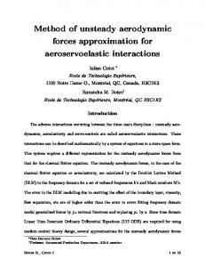
The present STG method takes 500 steps to converge, and exhibits a convergence rate similar to those of the steady flow solvers. The speed up of the STG solution over a direct unsteady solution using 200 physical time steps for this compressor stage is about 25 times. The instantaneous entropy contours are compared for the mid-span section as shown in Fig. 1. The signatures of the passages shock waves are clearly identifiable. The axial velocity contours at 90% span are shown in Fig. 2. It can be seen that the STG solution compares reasonably well with the direct solution. The close-up flow fields at 90% span (Fig. 2) shows that there is considerable separated flow on the rotor suction side around the shock foot due to the shock-boundary interaction. Also, the flow in the stator passages on the suction side is highly loaded and appears to be on the verge of separating. The steady solution like convergence for this case underlines the robustness of the present STG method for such highly loaded and sensitive flow regimes.

(a) Mixing-plane

(b) Frozen-rotor

(c) Direct unsteady

(d) Present (STG)

(a) Direct unsteady

(b) Present (STG)

Figure 2. Axial velocity contours at 90% span 2.2 Stator-Stator and Rotor-Rotor Clocking Effects For a two-stage turbomachinery configuration, the potential in gaining further performance by making use of the clocking between two relatively stationary blade rows is widely recognized. The associated multiple unsteady runs required (even for the same blading profiles) highlight the need for efficient unsteady flow methods for design applications. It is clear that effect of clocking is highly dependent on the blade counts of the two relatively stationary blade rows (e.g. as described by He et al [17]). The strongest clocking effect happens when the two relatively stationary rows have the same blade count. The convenient configuration for which the statorstator and rotor-rotor clocking potentials can both be explored would thus be a repeating 2-stage configuration with the same stator count and the same rotor count for both stages, whist the rotor and stator counts are taken to be different, at least for a typical aero-mechanical consideration. A repeating 2-stage configuration is thus set up. The second stage is essentially of the same configuration as the first. It is taken from the ¼ MT1 stage, with 8 stator and 15 rotor passages. Only quasi-3D solutions are examined, and the stream-tube height in the 3rd direction is varied to give a sensible axial velocity distribution to roughly match the relative flow angles to the corresponding blade angles. The STG calculations are carried out for 10 stator-stator clocking positions and 10 rotor-rotor clocking positions respectively. The hugely more time consuming direct unsteady calculations are only carried out for a couple of clocking positions for validation purposes. Stator-Stator clocking Fig.3 shows the instantaneous entropy contours for the 2stage configuration. There is clearly an excellent agreement between the two unsteady methods, serving the validation purposes. Impact of the clocking is mainly expected in the second stage. The time-averaged entropy contours for two clocking positions (for which the direct solutions are available) are shown in Fig.4. Excellent comparisons between the direct unsteady solution and the present STG are evident also for the

Figure 1. Instantaneous entropy contours at mid-span

3


time-averaged distributions. The time-mean flow in the second stator row is strongly affected by the clocking. Also noted is that the flow in the second rotor is visibly altered by the statorstator clocking as well. For turbine aerothermal performance, temperature distributions are of particular relevance to heat transfer and cooling designs. Here the interest is twofold, a)

is there a meaningful clocking dependence of the temperatures? b) can the STG method pick up any meaningful influence of clocking as adequately as the direct unsteady solution does?

Direct unsteady Present (STG) (a) reference clocking

Direct unsteady Present (STG) (b) 2nd stator clocked by 50% Pitch Figure 4. Time-averaged entropy contours (for 2 Stator-Stator clocking positions)

(a) Direct Unsteady

More relevantly, time-averaged blade surface temperatures on the second rotor and second stator are shown in Figs. 6-7 for different clocking positions. The surface fluid temperature can be roughly regarded the fluid driving temperature for convective heat transfer. It can be seen that the time-averaged temperatures over certain parts of blade surfaces can vary up to 1% TET when the two stators are clocked. 1% TET variation in blade surface temperatures should certainly be relevant to HP turbine blade durability. Again the direct solutions for the two clocking positons calculated agree very well with the corresponding STG solutions.

(b) Present (STG) Figure 3. Instantaneous entropy contours All temperatures presented are normalized by the turbine entry total temperature (TET). First, we look at the circumferential profiles of the time-averaged total temperatures at the 2-stage turbine exit as shown in Fig. 5. It shows that there is more than 1% TET of the temperature non-uniformity at the exit under certain clocking condition, but hardly any under some others (especially when clocked by 35% pitch). The comparison between the STG and the direct solutions shows excellent agreement, confirming the capability of the STG in capturing the clocking effects very accurately.

Figure 5. Exit time-averaged total temperature profiles for different Stator-Stator clocking positions

4


Rotor-Rotor clocking Similar to the stator-stator clocking analyzed, the rotorrotor clocking is now examined. Figure 9 shows a comparison in time-averaged entropy contours between two different rotor clocking positions. Even though the rotor blades ‘see’ all disturbances while rotating, the time-averaged contours record quite distinctive high entropy regions. Figure 10 shows the normalized blade surface temperatures on the 2nd rotor, illustrating that there are different patterns at different clocking positions. Importantly for the validation purposes, these differences are consistently picked up by the STG as by the direct solutions. Figure 11 shows the turbine exit total temperature distributions along pitch at different clocking positions. The rotor-rotor clocking results show a slightly larger range of temperature non-uniformity than that for the statorstator clocking (Fig. 5).

Figure 6. Time-averaged blade surface temperatures for different Stator-Stator clocking positions (2nd stator)

Figure 7. Time-averaged blade surface temperatures for different Stator-Stator clocking positions (2nd rotor) The dependence of the total-to-total efficiency (η) on the stator-stator clocking is compared in Fig. 8. The STG solution captures very well the change in the efficiency for the two clocking positions compared to the corresponding direct unsteady solutions. The solutions show a maximum 0.08% variation with clocking. This may be deemed as insignificant, though in typical realistic 3D configurations, a larger variation would be expected. Note also the non-sinusoidal curve of the variation in Fig. 8.

(a) reference clocking position

(b) 2nd rotor clocked 50% pitch

Figure 9. Spatial-averaged entropy contours for 2 Rotor-Rotor clocking positions

Figure 8. Total-to-total efficiencies for different Stator-Stator clocking positions

5


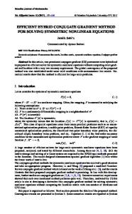
For blade aeromechanics, unsteady forcing is of primary interest. For a given rotor-rotor clocking, the STG method enables the unsteady pressures/forces to be evaluated by simply post-processing the spatial variations according to the clocking dependence as discussed before. Fig. 13 shows the equivalent time histories of tangential force on a blade in the second rotor row for 10 rotor-rotor clocking positions. The time-history results from the direct solutions for the two clocking positions calculated are also plotted (solid symbols), compared to the corresponding STG solutions (solid lines). Those for the axial forces are plotted in Fig. 14. It is clear that the clocking can lead to a difference in forcing magnitudes by about 50%. The clocking dependence behavior of the unsteady forcing is shown to be accurately and efficiently captured by the STG method.

Figure 10. Temperatures on second rotor surface for different Rotor-Rotor clocking positions

Figure 11. Exit time-averaged total temperature profiles for different Rotor-Rotor clocking positions In terms of the turbine efficiency, the result of the rotorrotor clocking, as shown in Fig. 12, can be contrasted to that for the stator–stator clocking (Fig. 8). The efficiency curve with the rotor-rotor clocking is of a smooth sinusoidal shape with only one peak. The percentage difference shows a maximum of 0.16% depending on the rotor-rotor clocking positions, which starts to be in the interested range for turbine design (bearing in mind again that the study is conducted for a quasi-3D configuration).

Figure 13. Time traces of unsteady Tangential forces for various Rotor-Rotor clocking (comparisons between direct and STG solutions are made for two clocking positions)

Figure 14. Time traces of unsteady Axial forces for various Rotor-Rotor clocking (comparisons between direct and STG solutions are made for two clocking positions)

Figure 12. Total-to-total efficiencies for different Rotor-Rotor clocking positions

6


nonlinearity. A general expression of such unsteadiness consisting of a finite number ND of periodic disturbances is given by He [4]:

Now we consider the computational efficiency of the STG method relative to the direct unsteady solution method. First note that a direct unsteady time marching/integration cannot self-start. The initial transients (numerical and/or physical) will need to take sufficiently long time to be ‘driven’ (propagated) out of the domain. This behavior can be regarded as a ‘history effect’. Therefore for the direct unsteady solution, if the computational cost is CDIR, the total costs for 10 clocking positions would be about 10CDIR. On the other hand, for the STG method, the major part of the cost for multi-clocking solutions is a single STG solution CSTG. Once a STG solution for the initial clocking position is obtained, rest of the calculations for other clocking positions can be obtained effectively as a sweep of these clocking positions (effectively a STG solution is self-starting without the ‘history effect’). Each subsequent solution can be restarted from a solution of a nearby clocking position, and converges very quickly, typically in 100~200 steps of the pseudo time marching. For the 10 clocking positions, the total costs of the STG solutions are practically equivalent to about 3-4CSTG. In the present calculations a single STG solution is about 38 times faster than a direct solution, i.e. CDIR = 38CSTG. Consequently, for 10 clocking positions, we roughly have (CDIR)10 clocking  100 (CSTG)10 clocking

𝑁𝐷

𝑈(𝑥, 𝑡) = 𝑈0 (𝑥) + ∑ 𝑈(𝑥, 𝑡)𝑖

(2)

𝑖=1

where U0 is the overall time mean, and each disturbance Ui has its own fundamental frequency fi and hence can be expanded further and expressed by a temporal Fourier series. The principal capability of the Fourier method for multiple unsteady disturbances in turbomachinery was demonstrated in a form of the generalized Shape-Correction by He [4], and Li and He [8]. The method is however slow in convergence due to the iterative corrections of the Fourier coefficients. The challenge for the STG method here is how to deal with multiple disturbances while having a steady solution convergence rate as intended. As far as the temporal gradient is concerned, it then follows: 𝑁𝐷

𝜕𝑈 𝜕𝑈𝑖 = ∑ 𝜕𝑡 𝜕𝑡

(3)

𝑖=1

In the context of the STG method, the temporal and spatial gradients are linked for a single disturbance with a relative rotating speed of  by:

(1)

Therefore the overall computational speed up of the STG is around 2 orders of magnitude compared to a direct solution. It should also be reminded that the speed-up discussed above is for 10 rotor-rotor clocking positions only (or for 10 stator-stator clocking positions only). The dependence of aerothermal performance on both rotor-rotor and stator-stator clocking as indicated so far means that the overall clocking design space for a given 2-stage blade geometry should cover 10x10 rotor-rotor and stator-stator clocking positions. Therefore, the implication of an efficient unsteady solution like the present STG method for the computational cost in blade clocking design analyses can be quite profound.

𝜕𝑈 𝜕𝑈 = ( ) (𝜔) 𝜕𝑡 𝜕𝜃

(4)

Then, Eq. 3 should be translated to (for a case with ND disturbances): 𝑁𝐷

𝜕𝑈 𝜕𝑈 = ∑( 𝜔)𝑖 𝜕𝑡 𝜕𝜃

(5)

𝑖=1

3.2 Superimposed Temporal Gradients The linear form of the general expression of multidisturbances (Eq. 2), and of those for the temporal gradients (Eq. 3, Eq. 4) in particular provides some motivation and justification for a simplified treatment. For instance, consider a single stage subject to an inlet temperature distortion (‘hot streak’). The linear form of the temporal gradients for the 2nd row should lead to a balanced unsteady equation (when converged with U/ ~ 0) in a form of

3. TREATMENT OF MULTIPLE DISTURBANCES 3.1 General Modelling Consideration Situations of unsteady flows in multiple blade rows of completely arbitrary blade counts are complex. But if the unsteadiness is dominated by those disturbances due bladerow interactions, the general clocking dependence as assumed in Part I should hold. In addition, a complex unsteady flow should be able to be decomposed into various periodic disturbances, each with a distinctive fundamental frequency (and its higher harmonics). A fundamental feature of multi-disturbance situations is that all disturbances are deterministic. Each can be traced back either to a primary disturbance, i.e. a bladerow interaction disturbance directly identifiable by clocking positioning relative to a blade, or to an ‘induced’ disturbance as a combination of several primary disturbances due to the

𝜕𝑈 𝜕𝑈 𝑅(𝑈) = − ( ) −( ) 𝜕𝑡 𝑖𝑛𝑙𝑒𝑡 𝜕𝑡 1𝑠𝑡 𝑟𝑜𝑤

(6)

A decomposed balancing considered here will resort to solving one disturbance first, e.g. the stage configuration with a clean inlet to get the corresponding temporal gradient for the second row:

7


𝜕𝑈 0 ( ) = −𝑅 (𝑈 1𝑠𝑡 ) 1𝑠𝑡 𝑟𝑜𝑤 𝜕𝑡 𝑟𝑜𝑤

a direct spatial Fourier transform should capture harmonics reflecting the sources of disturbances. Consider a three blade-row case, the difference in blade counts NIJ between row I and row J means that NIJ harmonic is a main harmonic from a target bladerow. A blade count difference between two rows clearly corresponds to the number of nodes of the disturbance in circumference, as illustrated by Li and He [8]. For instance, if the stator-stator count difference is two in a three-blade row configuration, the flow disturbances corresponding to the stator-stator interference has two repeating patterns circumferentially over the annulus. More specifically consider 32 passages in the first stator, followed by 61 rotor passages and then 39 passages in the second stator. In the second stator row, there should be only 19 harmonics maximum expected from the 39 sample points available. The blade count difference between the first and second row implies that the 7th spatial harmonic should result from the interaction between the current row (the 2nd stator) and the first stator. On the other hand, the 22nd spatial harmonic should be the main harmonic resulting from the interaction between the current row and the rotor immediately upstream, while this high harmonic number is beyond the limit set by the Nyquist criterion. As discussed earlier, the linear form of the temporal gradients for multiple disturbances means that if we can get the gradient for one of the two disturbances, we can solve the rest of the problem almost like a single disturbance one. In this case, the 7th harmonic is identified as the one for the interaction with the 1st stator. We can then use this harmonic and its 2nd harmonic (i.e. the 14th harmonic over the annulus) to approximate the gradient component for the interaction between the current row (2nd stator) and the 1st stator. For certain cases, it is possible to also get higher harmonics beyond that restricted by the Nyquist limit. Now we will need to make use of the aliasing. For the example considered, there are only by the maximum 19 circumferential harmonics nominally covered over the 39 passages. Now we would like to have information for the 21st harmonic (i.e. the 3rd harmonic of the 7th harmonic, which is the fundamental harmonic representing the stator-stator interaction as discussed above). Consider a spatial Fourier transform of Np points evenly spread over 2π annulus (j=1, 2,..Np)

(7)

Then if we assume that the contribution of this temporal gradient component for the 1st row remains the same in the case subject to the combined disturbances, then 𝜕𝑈

𝑅(𝑈) = − ( )

𝜕𝑡 𝑖𝑛𝑙𝑒𝑡

𝜕𝑈 0

− ( ) 1𝑠𝑡 𝜕𝑡

(8)

𝑟𝑜𝑤

In the framework of the STG method, the full unsteady equation during a pseudo time marching reads (similar to Eq. 7 of Part 1[1]), 𝜕𝑈 𝜕𝑈 𝜕𝑈 0 + 𝑅(𝑈) = − ( 𝜔) − ( 𝜔) 1𝑠𝑡 𝜕𝜏 𝜕𝜃 𝑖𝑛𝑙𝑒𝑡 𝜕𝜃

(9)

𝑟𝑜𝑤

Now, solving the problem under two disturbances is made equivalent to solving a single disturbance problem (i.e. that under the inlet disturbance only). Note particularly that the nonlinear flux terms (LHS of Eq. 8) will be in the exactly same form as the original equation (Eq. 6), for the multidisturbances. Note also that for the nonlinear flow equations, the bottom-line contribution of the temporal gradients is simply to provide a part to balance those nonlinear fluxes terms. The present treatment should be deemed to be adequate if the overall contribution of the temporal gradients is not strongly dependent on how the temporal gradient part of the first disturbance is obtained. The treatment described above is in some way similar to the technique adopted for the nonlinear harmonic balance solution by Frey et al. [12]. The key difference is that the present treatment makes no simplification of any sort at interfaces. All the temporal gradient summations are only applied for the temporal gradient parts of a linear form in balancing the unsteady equations of interior domain points. As will be shown by the computational results later, this technique of using summed temporal gradients works quite well for the cases tested. The main drawback is that this approach requires extra calculations from each extra disturbance. Nevertheless, for a stage configuration with inlet/exit disturbances, the solutions by using the summed temporal gradients technique are still shown to be by one order of magnitude faster than corresponding direct unsteady simulations.

𝜃𝑗 =

𝑗

𝑁𝑝

2𝜋

(10)

In order to consider a higher harmonic over that set by the Nyquist limit, noting the circular functions linking (Np-n) harmonic and n harmonic:

3.3 Spectral Filtering

𝑐𝑜𝑠 ((𝑁𝑝 − 𝑛)𝜃𝑗 ) = cos (𝑛

Frequency filtering is often used in spectral signal processing to retain wanted disturbances and remove unwanted ones. For certain blade counts, the frequency filtering can be simply and directly used for both the original blade passages in the physical domain and those sequenced after making use of the relative clocking of the passages. For the original passages,

𝑠𝑖𝑛 ((𝑁𝑝 − 𝑛)𝜃𝑗 ) = −sin (𝑛

8

𝑗

𝑁𝑝

2𝜋) = cos(𝑛𝜃𝑗 )

𝑗 2𝜋) = −sin(𝑛𝜃𝑗 ) 𝑁𝑝

(11)

(12)


solutions, but only 1.5% in the steady solutions, which is similar to that in a clean inflow case.

These relations effectively can be used to link the Fourier coefficients for the (Np-n)th harmonic and the nth harmonic, as they are aliased. For the case with 39 sample points, the 21st harmonic (the third sub-harmonic of the 7th) can be obtained from the 18th harmonic (i.e. 18=39-21) with a negative sign in the sine term only. Once the required harmonics are worked out for one disturbance, the original problem with two disturbances now effectively becomes one with one disturbance only, given the linear summative form of the temporal gradients (Eq. 2 and Eq. 3) It must be pointed out that the fundamental condition for the aliasing to represent any useful information is that the aliased harmonics will have to have no meaningful resident physical disturbances, which may not always be possible. Thus the harmonics worked out by making use of the aliasing as discussed above should be minimized or confined to higher harmonics whenever possible. The superimposed time gradient method introduced in the last section tends to be less restrictive.

(a) Mixing-plane

(b) Frozen-rotor

(c) Direct Unsteady

(d) Present (STG)

4 TEST CASES FOR MULTI-DISTURBANCES 4.1 Hot Streaks 2D HPT Stage Configuration A turbine stage with inlet temperature disturbances (hot streaks) is analyzed by the superimposed time gradient method described in Section 3.2. The ¼ annulus MT1 stage configuration is taken with 8 NGV and 15 rotor passages. The hot-streak has a ±50°K temperature range. A uniform inlet temperature used for a clean flow baseline case is 444°K. Two hot-streak length scales are considered. In the first case, the hot streak-NGV count ratio is 1:2. In the second case, the hot streak has a longer wave length covering 8 NGV passages (i.e. hot streak/NGV counts of 1/8). Figure 15 shows the comparison in instantaneous entropy contours among four solutions: the mixing-plane, the frozenrotor, the direct unsteady solution, and the proposed STG method. Clearly notable is the position of the hot-streaks at the stage exit. The frozen rotor solution appears to have similar profiles of high entropy at the exit plane to the direct unsteady and the present STG solutions, but the origins are clearly different. The unsteady transport of hot streaks and wakes shown in the direct unsteady solution is well captured by the STG solution. The frozen-rotor solution clearly could not get the right transport of the disturbances in rotor, and the mixingplane misses it completely. The STG method uses the superimposed temporal gradients technique is 14 times faster than the direct unsteady solution for this 2D to streak case. Figure 16 shows a comparison of time-averaged and passage-averaged total temperature profiles at the rotor exit. The present STG solution shows a very good agreement with the direct unsteady solution. The maximum temperature variation for the hot streak cases is around 3% in the unsteady

Figure 15. Instantaneous entropy contours for hot-streaks (hot streak/NGV counts: 1/2)

Figure 16. Circumferential distributions of time-averaged total temperatures at exit (hot streak/NGV counts: 1/2) The total-to-total efficiency of the turbine stage is calculated and the percentage differences are compared as

9


shown in Table 1. While the present solution and the direct unsteady solution shows almost identical values, the difference in the efficiency between the mixing-plane solution and the unsteady reference value is more than 1%. This level of difference is certainly quite significant to blade design, though bearing in mind the 2D nature of this case. Table 1. Total-to-total efficiency (2D hot streak case) Method  (%)

Mixing plane -1.11

Frozen rotor +0.55

Direct Unsteady reference

Present (STG) -0.01

(a) Mixing plane

Now we turn to the case with a longer hot-streak lengthscale in the circumferential direction (hot-streak / NGV counts of 1/8). The magnitude of the inlet temperature distortion is kept the same as the previous hot streak case with the shorter scale. The interest here is to identify the impact of circumferential length scale and the ability of the present STG method in capturing it. Some previous work has indicated that there can be a strong dependence of blade aerothermal responses to inlet hot streak length scale (hot streak/NGV counts) [19]. The instantaneous temperature profiles at the stage exit are shown in Fig. 17. The entropy contours are compared as shown in Fig. 18. It is known that the strength of axial propagation of a disturbance is linked to its circumferential length scale. Thus a larger scale unsteady disturbance (though at a lower frequency) is expected in this case as shown. Fig.17 can be very usefully contrasted to Fig.16. Both are the temperature profiles at the stage exit, having the same magnitude in the inlet temperature distortion. The profound impact of the circumferential length scale on the axial propagation of the inlet disturbances is clearly demonstrated. Again for the case, the STG method is shown to work very well for this long length scale hot streak case. The STG method for this longer hot-streak length-scale is 11 times faster than the direct unsteady solution.

(c) Direct Unsteady

(b) Frozen rotor

(d) Present (STG)

Figure 18. Instantaneous entropy contours for long scale hot-streak (hot streak/NGV counts: 1/8) 3D HPT stage configuration with rotor tip clearance A further case is added to illustrate the predictive capability of the proposed STG method for a 3D HPT stage configuration subject to hot streaks. For this 3D case, a realistic hot streak/NGV count ratio of 1: 2 is taken. The original quarter annulus MT1 stage is adopted (8 NGV and 15 rotor passages). The given hot streak and blade counts correspond to the case with 4 hot-streak/NGV passage groups on one side and 15 rotor passages on the other side. The STG sequencing of the 15 rotor passages is conducted against four of ‘stator’ groups (each having 1 hot streak and 2 NGV passages). The hot-streak has the ±50°K temperature range from 400°K to 500°K. The stage domain of 23 blade passages is meshed with 27 million mesh nodes in total. The rotor blades have a 0.5% tipclearance. In terms of the computational cost, the STG solution is 37 times faster than the direct unsteady solution, using the same number of computer processing cores. The instantaneous entropy contour plots for the mid-span are presented in Fig. 19. The mixing-plane and the frozen rotor solutions clearly are unable to capture unsteady wake propagations. Three-dimensional and highly complex vortical flow interactions in rotor passages are also well captured by the

Figure 17. Circumferential distributions of instantaneous total temperatures at exit (hot streak/NGV counts: 1/8)

10


STG solution. The static temperature contours near the rotor tip (at 90% span, Fig. 20) indicate the impact of tip clearance flow, with noticeable signatures of the tip leakage vortices. The timeaveraged entropy contours at the exit plane are shown in Fig. 21. Similar to the stage solution under a clean inlet as discussed in Part I [1], the tip-leakage vortex is weakened by the unsteadiness as indicated by both the present STG solution and the direct unsteady solution, in contrast to the mixing-plane solution. Hot-streak cores of the unsteady solutions show a shifted position and considerably more temperature smearing because of the mixing caused by unsteady hot streaks and NGV wakes. Mixing plane

Frozen rotor

Direct unsteady

Present (STG)

Figure 20. Instantaneous temperatures at 90% span

(a) Mixing plane (a) Mixing plane

(b) Frozen rotor (b) Frozen rotor

(c) Direct unsteady

(c) Direct unsteady

(d) Present (STG)

(d) Present (STG)

Figure 19. Instantaneous entropy contours at mid-span Table 2 shows the differences in the predicted total-to-total efficiency relative to the direct solution. About 0.5% difference in the stage efficiency results from the use of the mixing-plane in this case, which should certainly be of practical interest.

Figure 21. Time-averaged entropy contours at exit

4.2 Three-row Configurations with Non-equal Counts Consider now a 3-bladerow configuration on a 2D section. There are 32 stator blades in the 1st row, 61 rotor blades in the second and 39 stators in the third row. We use this configuration to test the solution capability of the spectral

Table 2. Total-to-total efficiency (3D hot streak) Method  (%)

Mixing plane -0.51

Frozen rotor +0.42

Direct Unsteady reference

Present (STG) +0.01

11


filtering technique. In this case spectral analyses show that at least three harmonics for each disturbance can be retained. Unsteady entropy contours are shown in Fig. 22 in which four methods are compared, (a) mixing plane, (b) frozen rotor, (c) direct unsteady and (d) the present approach. The signatures of unsteady wake migration and chopping by the relatively rotating blade rows are well captured. The present STG solution is shown to be compatible to the direct unsteady solution, and is qualitatively different from the two steady flow solutions. The time-averaged total temperatures at the 3-row domain exit are compared as shown in Fig. 23. The pattern of the present STG solution follows closely that of the direct unsteady solution and both show similar fluctuations, though details do differ. The STG solution is clearly much better than the mixingplane and the frozen-rotor solutions. The mixing-plane solution shows only one small peak for the 3rd blade row while losing the wakes from the 1st and 2nd blade rows. The frozen rotor solution shows much larger fluctuations caused by non-realistic upstream wake convections without sufficient mixing. The figure also clearly shows that the time-averaged total temperatures from both unsteady solutions are consistently lower than that of the steady mixing-plane, by around 0.5%, corresponding to a non-negligible difference in efficiency.

(a) Mixing-plane

(b) Frozen-rotor

(c) Direct unsteady

(d) Present (STG)

Figure 23. Circumferential distributions of time-averaged total temperatures (Stator-Rotor-Stator counts: 32-61-39) The time-averaged entropy comparison is shown in Fig. 24. The high entropy regions in the 2nd and 3rd rows caused by the 1st stator blade row are well captured by both unsteady solutions. Given that the high entropy regions can correspond to those with high temperatures, these regions are also quite relevant to blade thermal designs. This point is highlighted in the blade surface temperature profiles, shown in Figs. 25-27. It can be seen that about 1% temperature differences (measured in terms of TET) exist on the rotor suction surface between the direct unsteady and the mixing-plane solutions. The two solutions also show about 0.5% TET difference on the surfaces of the 2nd stator blade. All the corresponding STG results show better agreement with the direct unsteady solution than the steady solutions. These results demonstrate the potential of the developed capability for capturing multi-disturbance effects, and very encouraging, particularly given that resolving multidisturbances has been a very challenging modelling aspect for reduced/truncated unsteady turbomachinery flow methods.

(a) Direct unsteady

Figure 22. Comparison of instantaneous entropy contour (Stator-Rotor-Stator counts: 32-61-39)

(b) Present (STG)

Figure 24. Time-averaged entropy contours (Stator-Rotor-Stator counts: 32-61-39)

12


the present STG solutions are compared with the direct unsteady solution counterparts. The convergence characteristics of all STG solutions are shown to be comparable to those of the steady frozen rotor solutions. A very highly loaded transonic compressor stage case underlines the robustness of the STG method for separating flow conditions subject to strong adverse pressure gradients. The results of the 2-stage turbine configuration indicate a notable clocking dependence of blade surface time-mean temperatures. It is also illustrated that there is considerable further potential in speed-ups compared to the conventional direct unsteady solutions, if design optimizations utilize both the stator-stator and the rotor-rotor clocking. Several numerical techniques are introduced to deal with multiple unsteady disturbances. The developed capabilities have been tested for 2D and 3D stage configurations with inlet hot streak disturbances, and for a 3-bladerow turbine configuration with non-equal blade counts. The calculated results by the present STG method all compare well with those of the direct unsteady solutions, while giving at least one order of magnitude computational speed up.

Figure 25. Time-averaged surface temperatures (1st stator) (Stator-Rotor-Stator counts: 32-61-39)

ACKNOWLEDGMENT The authors would like to thanks Rolls-Royce and UK Technology Strategy Board (TSB) for funding the work and the permission to publish the paper.

Figure 26. Time-averaged surface temperatures (rotor) (Stator-Rotor-Stator counts: 32-61-39)

REFERENCES [1] J. Yi and L. He, “Space-Time Gradient Method for Unsteady Bladerow Interaction – Part I: Basic Methodology and Verification”, ASME 2015 Turbo Expo, ASME Paper No. GT 2015-43152. [2] J. D. Denton, 1992, “The Calculation of ThreeDimensional Viscous Flow through Multistage Turbomachines”, J. Turbomach., 114(1), pp. 18-26.

Figure 27. Time-averaged surface temperatures (2nd stator) (Stator-Rotor-Stator counts: 32-61-39)

[3] L. He, 2010, “Fourier Method for Turbomachinery Application”, Progress in Aerospace Sciences, 46, pp. 329-341.

CONCLUSION

[4] L. He, 1992, “A Method of Simulating Unsteady Turbomachinery Flows with Multiple Perturbations”, AIAA J., 30(12), pp. 2730-27350.

A new space-time gradient (STG) method has been developed with the basic intent to maintain as many modelling fidelities of a direct unsteady method as possible while achieving a significant speed-up. In particular, a fully conservative rotor-stator interface treatment is adopted, as in the direct unsteady solution. The methodology and some preliminary verification are presented in Part I [1]. In this paper as Part II, we present further validations and case study applications to examine and demonstrate capabilities and ranges of the applicability of the method. All the results of

[5] W. Ning and L. He, 1998, “Computation of Unsteady Flows around Oscillating Blades Using Linear and Nonlinear Harmonic Euler Methods”, J. Turbomach., 120(3), pp. 508-514. [6] K. C. Hall, J. P. Thomas, W. S. Clark, 2002, “Computation of Unsteady Nonlinear Flows in Cascade Using a Harmonic Balance Technique”, AIAA J., 40(5), pp. 879886.

13


[7] G. A. Gerolymos, G. J. Michon and J. Neubauer, 2002, “Analysis and Application of Chorochronic Periodicity in Turbomachinery Rotor/Stator Interaction Computations”, J. Propul. Power, 18(6), pp. 1139-1152. [8] H. D. Li and L. He, 2005, “Toward Intra-Row Gap Optimization for One and Half Stage Transonic Compressor”, J. Turbomach., 127(3), pp. 589-598. [9] S. Vilmin, E. Lorrain, C. H. Hirsch and M. Swoboda, 2006, “Unsteady Flow Modeling Across the Rotor/Stator Interface Using the Nonlinear Harmonic Method”, ASME 2006 Turbo Expo, 6, ASME Paper No. GT 2006-90210. [10] K. Ekici and K. C. Hall, 2007, “Nonlinear Analysis of Unsteady Flows in Multistage Turbomachines Using Harmonic Balance”, AIAA J., 45(5), pp. 1047-1057. [11] F. Sicot, G. Dufour and N. Gourdain, 2011, “A TimeDomain Harmonic Balance Method for Rotor/Stator Interactions”, J. Turbomach., 134(1), pp. 011001-01100113. [12] C. Frey, G. Ashcroft, H.-P. Kersken and C. Volgt, 2014, “A Harmonic Balance Technique for Multistage Turbomachinery Applications”, ASME 2014 Turbo Expo, 2B, ASME Paper No. GT 2014-25230, pp. V02BT39A005 [13] D. J. Dorney and O. P. Sharma, 1997, “Evaluation of Flow Field Approximations for Transonic Compressor Stages”, J. Turbomach., 119(3), pp. 445-451. [14] W. Höhn, R. Gombert and A. Kraus, 2001, “Unsteady Aerodynamical Blade Row Interaction in a New Multistage Research Turbine: Part 2 – Numerical Investigation”, ASME 2001 Turbo Expo, 1, ASME Paper No. 2001-GT-0307, pp. V001T03A011. [15] N. Billiard, V. J. Fidalgo, R. Dénos and G. Paniagua, 2007, “Analysis of Stator-Stator Clocking in a Transonic Turbine”, ASME 2007 Turbo Expo, 6, ASME Paper No. GT-2007-27323. [16] N. Billiard, G. Paniagua, and R. Dénos, 2008, “Impact of Clocking on the Aero-Thermodynamics of a Second Stator Tested in a One and a Half Stage HP Turbine”, J. Therm. Sci., 17(2), pp. 97-110. [17] L. He, T. Chen, R. G. Wells, Y. S. Li and W. Ning, 2002, “Analysis of Rotor-Rotor and Stator-Stator Interferences in Multi-Stage Turbomachines”, J. Turbomach., 124(4), pp. 564-571. [18] L. Reid and R. D. Moore, 1978, “Design and Overall Performance of Four Highly Loaded, High-Speed Inlet Stages for an Advanced High-Pressure-Ratio Core Compressor”, NASA Technical Report, NASA-TP-1337. [19] L. He, V. Menshikova and B. R. Haller, 2007, “Effect of Hot-Streak Counts on Turbine Blade Heat Load and Forcing”, J. Propul. Power, 23 (6), pp1235-1241.

14
