SPARSE AND LOW-RANK MATRIX DECOMPOSITION VIA ALTERNATING DIRECTION METHODS XIAOMING YUAN∗ AND JUNFENG YANG† Abstract. The problem of recovering the sparse and low-rank components of a matrix captures a broad spectrum of applications. Authors in [4] proposed the concept of ”rank-sparsity incoherence” to characterize the fundamental identifiability of the recovery, and derived practical sufficient conditions to ensure the high possibility of recovery. This exact recovery is achieved via solving a convex relaxation problem where the l1 norm and the nuclear norm are utilized for being surrogates of the sparsity and low-rank. Numerically, this convex relaxation problem was reformulated into a semi-definite programming (SDP) problem whose dimension is considerably enlarged, and this SDP reformulation was proposed to be solved by generic interior-point solvers in [4]. This paper focuses on the algorithmic improvement for the sparse and low-rank recovery. In particular, we observe that the convex relaxation problem generated by the approach of [4] is actually well-structured in both the objective function and constraint, and it fits perfectly the applicable range of the classical alternating direction method (ADM). Hence, we propose the ADM approach for accomplishing the sparse and low-rank recovery, by taking full exploitation to the high-level separable structure of the convex relaxation problem. Preliminary numerical results are reported to verify the attractive efficiency of the ADM approach for recovering sparse and low-rank components of matrices. Key words. Matrix decomposition, sparse, low rank, alternating direction method, l1 norm, nuclear norm. AMS subject classifications. 90C06, 90C22,90C25,90C59, 93B30
1. Introduction. Matrix representations of complex systems and models arising in various areas often have the character that such a matrix is composed of an sparse matrix and an low-rank matrix. Such applications include the model selection in statistics, system identification in engineering, partially coherent decomposition in optical systems, and matrix rigidity in computer science, see e.g. [15, 16, 17, 30, 35, 37, 41]. To better understand its behavior and properties and to track it more efficiently, it is of significant interest to take advantage of the decomposable character of such a complex system. One necessary way towards this goal is to recover the sparse and low-rank components of the corresponding given matrix, but without no prior knowledge about the sparsity pattern or the rank information. Despite its powerful applicability, the problem of sparse and low-rank matrix decomposition (SLRMD) was highlighted and intensively studied only very recently by [4]. Obviously, the SLRMD problem is in general ill-posed (NP-hard) and thus not trackable. In sprit of the influential work of [5, 6, 9, 10, 11, 36] in the areas of compressed sensing and statistics, authors of [4] insightfully proposed the concept of ”rank-sparsity incoherence” to characterize the fundamental identifiability of the recovery of sparse and low-rank components. Accordingly, a simple deterministic condition for the eligibility of exact recovery was derived therein. Note that the concept of ”rank-sparsity incoherence” relates algebraically the sparsity pattern of a matrix and its row or column spaces via an uncertainty principle. Throughout, we assume by default that the matrix under consideration is recoverable for sparse and ∗ DEPARTMENT OF MATHEMATICS, HONG KONG BAPTIST UNIVERSITY, HONG KONG, CHINA (
[email protected]). THIS AUTHOR WAS SUPPORTED BY THE RGC GRANT 203009 AND THE NSFC GRANT 10701055. † DEPARTMENT OF MATHEMATICS, NANJING UNIVERSITY, NANJING, JIANGSU, CHINA (
[email protected]).
1
2
X. M. YUAN and J. F. YANG
low-rank components. By realizing the widely-used heuristics of using the l1 -norm as the proxy of sparsity and the nuclear norm as the surrogate of low-rank in many areas such as statistics and image processing (see e.g. [6, 8, 14, 36]), authors of [4] suggested to accomplish the sparse and low-rank recovery by solving the following convex optimization problem: minA,B γkAkl1 + kBk∗ s.t. A + B = C,
(1.1)
where C ∈ Rm×n is the given matrix to be recovered; A ∈ Rm×n is the sparse component of C; B ∈ Rm×n is the low-rank component of C; k · kl1 is the l1 norm defined by the component-wise sum of absolute values of all entries; k · k∗ is the nuclear norm defined by the sum of all singular values; and γ > 0 is a constant providing a trade-off between the sparse and low-rank components. Let A∗ and B ∗ be the true sparse and low-rank components of C which are to be recovered. Then, some conditions on A∗ and B ∗ were proposed in [4] to ensure sufficiently that the unique solution of (1.1) is exactly (A∗ , B ∗ ) for a range of γ, i.e., the exact spare and low-rank recovery of C can be accomplished. We refer to Theorem 2 in [4] for the delineation of these conditions, and we emphasize that these conditions are practical as they are satisfied by many real applications, see also [4]. Therefore, efficient numerical solvability of (1.1) becomes crucial for the task of recovering the sparsity and low-rank components of C. In particular, it was suggested in [4] to apply some interior-point solvers such as SDPT3 [40] to solve the semi-definite programming (SDP) reformulation of (1.1). For many cases, however, matrices to be decomposed are large-scale in dimensions, and it is not hard to imagine that this large-scale feature significantly aggrandizes the difficulty of recovery. In fact, it has been well realized that the interior-point approach is numerically invalid for largescale (actually, even for medium-scale) optimization problems with matrix variables. In particular, for solving (1.1) via the interior-point approach in [4], the dimension of the SDP reformulation is even magnified considerably compared to that of (1.1), see (A.1) in [4]. Hence, just as what authors of [4] raised at the end, it is of particular interest to develop efficient numerical algorithms for solving (1.1) in order to accomplish the recovery of sparse and low rank components, especially for large-scale matrices. For doing so, we observe that (1.1) is well-structured in the sense that the separable structure emerges in both the objective function and the constraint. Thus, we have no reasons not to take advantage of this favorable structure for the sake of algorithmic design. Recall that (1.1) was regarded as a generic convex problem, and its beneficial structure was completely ignored in [4]. In fact, the high-level separable structure of (1.1) can be readily exploited by the well-known alternating direction method (ADM). Thus, we are devoted to presenting the ADM approach for solving (1.1) by taking full advantage of its beneficial structure. The rationale of making use of the particular structure of (1.1) for algorithmic sakes also conforms to what Nesterov has illuminated in [33]: ”It was becoming more and more clear that the proper use of the problem’s structure can lead to very efficient optimization methods......”. As we will analyze in detail, the ADM approach is attractive for sparse and low-rank recovery because that the main computational load of each iteration is dominated by only one singular value decomposition of B. 2. The ADM approach. Generally speaking, ADM is a practical improvement of the classical Augmented Lagrangian method for solving convex programming
Sparse and Low-Rank Matrix Decomposition via ADM
3
problem with linear constraints, by fully taking advantage of its high-level separable structure. We refer to the wide applications of ADM in many areas such as convex programming, variational inequalities and image processing, see, e.g., [2, 7, 12, 13, 18, 19, 20, 21, 22, 24, 28, 39]. In particular, novel applications of ADM for solving some interesting optimization problems have been discovered very recently, see e.g. [13, 25, 32, 43, 44]. The Augmented Lagrangian function of (1.1) is L(A, B, Z) := γkAkl1 + kBk∗ − hZ, A + B − Ci +
β kA + B − Ck2 , 2
where Z ∈ Rm×n is the multiplier of the linear constraint; β > 0 is the penalty parameter for the violation of the linear constraint and h·i denotes the standard trace inner product and k · k is the induced Frobenius norm. Obviously, the classical Augmented Lagrangian method (see e.g. [1, 34]) is applicable, and its iterative scheme is: ½ (Ak+1 , B k+1 ) ∈ argminA,B∈Rm×n {L(A, B, Z k )}, (2.1) Z k+1 = Z k − β(Ak+1 + B k+1 − C), where (Ak , B k , Z k ) is the given triple of iterate. The direct application of the Augmented Lagrangian method, however, treats (1.1) as a generic minimization problem and ignores its favorable separable structure emerging in both the objective function and the constraint. Hence, the variables A and B are minimized simultaneously in (2.1). Indeed, this ignorance of the direction application of Augmented Lagrangian method for (1.1) can be made up by the well-known ADM method which minimizes the variables A and B serially. More specifically, the original ADM (see e.g. [19, 20, 21, 22]) solves the following problems to generate the new iterate: k+1 ∈ argminA∈Rm×n {L(A, B k , Z k )}, A k+1 B ∈ argminB∈Rm×n {L(Ak+1 , B, Z k )}, k+1 Z = Z k − β(Ak+1 + B k+1 − C), which is equivalent to 0 ∈ γ∂(kAk+1 kl1 ) − [Z k − β(Ak+1 + B k − C)].
(
0 ∈ ∂(kB Z
k+1
k+1
k
k+1
k∗ ) − [Z − β(A k
k+1
= Z − β(A
+B
+B
k+1
k+1
− C)].
− C),
(2.2a) (2.2b) (2.2c)
where ∂(·) denotes the subgradient operator of a convex function. We now elaborate on strategies of solving the subproblems (2.2a) and (2.2b). First, we consider (2.2a), which turns out to be the widely-used shrinkage problem (see e.g [38]). In fact, (2.2a) can be solved easily with explicit solution: Ak+1 =
1 k 1 Z − B k + C − PΩγ/β [ Z k − B k + C], ∞ β β
where PΩγ/β denotes the Euclidean projection onto ∞
n×n Ωγ/β | − γ/β ≤ Xij ≤ γ/β}. ∞ := {X ∈ R
4
X. M. YUAN and J. F. YANG
For the second subproblem (2.2b), it is easy to verify that it is equivalent to the following minimization problem: © ª 1 β B k+1 = argminB∈Rm×n kBk∗ + kB − [C − Ak+1 + Z k ]k2 . 2 β
(2.3)
Then, according to [3, 31], B k+1 admits the following explicit solution: B k+1 = U k+1 diag(max{σik+1 −
1 , 0})(V k+1 )T , β
where U k+1 ∈ Rm×r , V k+1 ∈ Rn×r are obtained via the singular value decomposition of C − Ak+1 + 1β Z k : C − Ak+1 +
1 k Z = U k+1 Σk+1 (V k+1 )T β
with Σk+1 = diag({σik+1 }ri=1 ).
Based on aforementioned analysis, we now delineate the procedure of applying ADM to solve (1.1). For given (Ak , B k , Z k ), the ADM takes the following schemes to generate the new iterate: Algorithm: the ADM for SLRMD problem: Step 1. Generate Ak+1 : Ak+1 =
1 k 1 Z − B k + C − PΩγ/β [ Z k − B k + C]. ∞ β β
Step 2 Generate B k+1 : B k+1 = U k+1 diag(max{σik+1 −
1 , 0})(V k+1 )T , β
where U k+1 , V k+1 and {σik+1 } are generated by the singular values decomposition of C − Ak+1 + 1β Z k , i.e., C − Ak+1 +
1 k Z = U k+1 Σk+1 (V k+1 )T , with Σk+1 = diag({σik+1 }ri=1 ). β
Step 3. Update the multiplier: Z k+1 = Z k − β(Ak+1 + B k+1 − C). Remark 1. It is easy to see that when the ADM approach applied to solve (1.1), the computation load of each iteration is dominated by one singular values decomposition (SVD) with the complexity O(n3 ), see e.g. [23]. In particular, existing subroutines for efficient SVD (e.g. [29, 31]) guarantees the efficiency of the proposed ADM approach for sparse and low-rank recovery of large-scale matrices. Remark 2. Some more general ADM methods are easy to be extended to solve the SLRMD problem. For example, the general ADM proposed by Glowinski [21, 22] which modifies Step 3 of the original ADM with a relaxation parameter in the interval √ (0, 5+1 2 ); and the ADM-based descent method developed in [42]. We here omit details of these general ADM type methods for succinctness. Convergence of ADM type methods are available in the literatures, e.g., [19, 20, 21, 22, 26, 42].
Sparse and Low-Rank Matrix Decomposition via ADM
5
Remark 3. The penalty parameter β is eligible for dynamic adjustment. We refer to, e.g., [24, 26, 27, 28], for the convergence of ADM with dynamically-variable parameter and some concrete effective strategies of adjusting this parameter. 3. Numerical results. In this section, we present experimental results to show the efficiency of ADM when applied to (1.1). Let C = A∗ + B ∗ be the available data, where A∗ and B ∗ are, respectively, the original sparse and low-rank matrices that we wish to recover. For convenience, we let γ = t/(1 − t) so that problem (1.1) can be equivalently transformed to min {tkAkl1 + (1 − t)kBk∗ : A + B = C} . A,B
(3.1)
The advantage of the reformulation in the form of (3.1) is that parameter t changes ˆt ) be a in a finite interval (0, 1) as compared to γ ∈ (0, +∞) in (1.1). We let (Aˆt , B numerical solution of (3.1) obtained by ADM. We will measure the quality of recovery by relative error to (A∗ , B ∗ ), which is defined as RelErr ,
ˆt ) − (A∗ , B ∗ )kF k(Aˆt , B , k(A∗ , B ∗ )kF + 1
(3.2)
where k · kF represents the Frobenius norm. All experiments were performed under Windows Vista Premium and MATLAB v7.8 (R2009a) running on a Lenovo laptop with an Intel Core 2 Duo CPU at 1.8 GHz and 2 GB of memory. 3.1. Experimental settings. Given a small constant τ > 0, we define ˆt − B ˆt−τ kF . difft , kAˆt − Aˆt−τ kF + kB
(3.3)
ˆt approaches zero matrix as t does. On the other hand, Aˆt approaches It is clear that B zero matrix as t becomes close to 1. Therefore, difft is stabilized on the boundaries of (0, 1). As suggested in [4], a suitable value of t should result to a recovery such that difft is stabilized and meanwhile t stays away from both 0 and 1. To determine a suitable value of t, we set τ = 0.01 in (3.3), which, based on our experimental ˆt ) with respect to results, is sufficiently small for measuring the sensitivity of (Aˆt , B t, and ran a set of experiments with different combinations of sparsity ratios of A∗ and ranks of B ∗ . In the following, r and spr represent, respectively, matrix rank and sparsity ratio. We tested two types of sparse matrices: impulsive and Gaussian sparse matrices. The MATLAB scripts for generating matrix C are as follows: • B = randn(m,r)*randn(r,n); mgB = max(abs(B(:))); • A = zeros(m,n); p = randperm(m*n); L = round(spr*m*n); – Impulsive sparse matrix: A(p(1:L)) = mgB.*sign(randn(L,1)); – Gaussian sparse matrix: A(p(1:L)) = randn(L,1); • C = A + B. Specifically, we set m = n = 100 and tested (r, spr) = (1, 1%), (2, 2%), . . . , (20, 20%), for which the decomposition problem roughly changes from easy to hard. Based on our experimental results, suitable values of t shrinks from [0.05, 0.2] to [0.09, 0.1] as (r, spr) increases from (1, 1%) to (20, 20%). Therefore, we set t = 0.1 in our experiments. In the following, we present experimental results for the two types of sparse matrices. In all experiments, we set m = n = 100. We simply set β = 0.25mn/kCk1 and terminated ADM when the relative change falls below 10−6 , i.e., RelChg ,
k(Ak+1 , B k+1 ) − (Ak , B k )kF ≤ 10−6 . k(Ak , B k )kF + 1
(3.4)
6
X. M. YUAN and J. F. YANG
3.2. Exact recoverability. In this section, we present numerical results to demonstrate exact recoverability of model (3.1). For each pair (r, spr), we ran 50 trials and claimed successful recoverability when RelErr ≤ ² for some ² > 0. The probability of exact recovery is the defined as the successful recovery rate. The following results show the recoverability of (3.1) for r varies from 1 to 40 and spr from 1% to 35%. Recoverability. RelErr ≤ 10−6
Recoverability. RelErr ≤ 10−5
Recoverability. RelErr ≤ 10−3 1
0.9
10
0.7 0.6
15
0.5
20
0.4 0.3
25
0.2
30 20 Rank
30
0.7 0.6
15
0.5
20
0.4
25
0.3
0.9
0.2
0.8
10
0.7 0.6
15
0.5
20
0.4
25
0.3 0.2
30
0.1
35
0
10
10
30
0.1
35
0.8
5 Sparsity Ratio (%)
0.8
1
0.9
5 Sparsity Ratio (%)
Sparsity Ratio (%)
5
40
0.1
35
0
10
20 Rank
30
40
0
10
20 Rank
30
40
Fig. 3.1. Recoverability results from impulsive sparse matrices. Number of trials is 50.
Recoverability. RelErr ≤ 10−4
Recoverability. RelErr ≤ 10−3
Recoverability. RelErr ≤ 10−2 1
0.5
15
0.4
20
0.3
25
0.2
30
0.1
Sparsity Ratio (%)
Sparsity Ratio (%)
10
1
0.9
5
0.8
10
0.7 0.6
15
0.5
20
0.4
25
0.3 0.2
30
0.9
5 Sparsity Ratio (%)
0.6
5
0.8
10
0.7 0.6
15
0.5
20
0.4
25
0.3 0.2
30
0.1
35
35 10
20 Rank
30
40
0
10
20 Rank
30
40
0.1
35
0
10
20 Rank
30
40
Fig. 3.2. Recoverability results from Gaussian sparse matrices. Number of trials is 50.
It can be seen from Figures 3.1 and 3.2 that model (3.1) shows exact recoverability when either the sparsity ratio of A∗ or the rank of B ∗ are suitably small. Specifically, for impulsive sparse matrices, the resulting relative errors are as small as 10−5 for a large number of test problems. When r is small, say r ≤ 5, ADM applied to (3.1) results to faithful recoveries with spr as high as 35%, while, on the other hand, high accuracy recovery is attainable for r as high as 30 when spr ≤ 5%. Comparing Figures 3.1 and 3.2, it is clear that, under the same conditions of sparsity ratio and matrix rank, the probability of high accuracy recovery is smaller when A∗ is Gaussian sparse matrices, which is quite reasonable since impulsive errors are generally easier to be eliminated than Gaussian errors. 3.3. Recovery results. In this section, we present two classes of recovery results on both impulsive and Gaussian sparse matrices. Figure 3.3 shows the results of 100 trials for several pairs of (r, spr), where x-axes represent the resulting relative errors (average those relative errors fall into [10−(i+1) , 10−i ]) and y-axes represent the number of trials ADM obtains relative errors in a corresponding interval. It can be seen from Figure 3.3 that, for impulsive sparse matrices (plot on the left), the resulting relative errors are mostly quite small and poor quality recovery appears for less than 20% of the 100 random trials. In comparison, for Gaussian sparse matrices (plot on the right), the resulting relative errors are mostly between 10−3 and 10−4 ,
7
Sparse and Low-Rank Matrix Decomposition via ADM
and it is generally rather difficult to obtain higher accuracy unless both r and spr are quite small. Impulsive sparse matrix
Gaussian sparse matrix
60
100
(r,spr) = (5, 30%) (r,spr) = (10,25%) (r,spr) = (15,15%) (r,spr) = (20,10%)
50
90 80 70
Count #
40
Count #
(r,spr) = (1, 5%) (r,spr) = (5, 5%) (r,spr) = (10,5%) (r,spr) = (10,1%)
30
60 50 40
20 30 20
10
10
0 −7 10
−6
10
−5
10
−4
10
Relative Error
−3
10
−2
10
−1
10
0 −7 10
−6
10
−5
10
−4
10
−3
10
Relative Error
Fig. 3.3. Recovery results of 100 trials. Left: results of impulsive sparse matrices; Right: results of Gaussian sparse matrices. In both plots, x-axes represent relative error of recovery (average those relative errors fall into [10−(i+1) , 10−i )) and y-axes represent the number of trials ADM results to a relative error in a corresponding interval.
In Figures 3.4 to 3.7, we present two results for each type of sparse matrices, where the rank of B ∗ , the sparsity ratio of A∗ , the number of iterations used by ADM, the resulting relative errors to A∗ , B ∗ (defined in a similar way as in (3.2)) and the total relative error RelErr defined in (3.2) are given in the captions. The sparsity ratios and matrix ranks used in all these tests are near the boundary of high accuracy recovery, which can be seen in Figures 3.1 and 3.2. From these results, it can be seen that high accuracy is attainable even for the boundary cases of high accuracy recovery. It is also implied that problem (3.1) is usually much easier to solve when C is corrupted by impulsive sparse errors as compared to Gaussian errors.
8
X. M. YUAN and J. F. YANG
True Sparse
Recovered Sparse
True Low−Rank
Recovered Low−Rank
Fig. 3.4. Results #1 from impulsive sparse matrix. Rank: 10, sparsity ratio: 20%, number of iteration: 39, relative error in sparse matrix: 1.06 × 10⁻⁶ , Relative error in low rank: 2.22 × 10⁻⁶ , relative error in total: 1.33 × 10⁻⁶ .
True Sparse
Recovered Sparse
True Low−Rank
Recovered Low−Rank
Fig. 3.5. Results #2 from impulsive sparse matrix. Rank 20, sparsity ratio: 10%, number of iteration: 45, relative error in sparse matrix: 1.55 × 10⁻⁶ , relative error in low rank: 1.79 × 10⁻⁶ , relative error in total: 1.63 × 10⁻⁶ .
Sparse and Low-Rank Matrix Decomposition via ADM
True Sparse
Recovered Sparse
True Low−Rank
Recovered Low−Rank
9
Fig. 3.6. Results #1 from Gaussian sparse matrix. Rank 10, sparsity ratio: 20%, number of iteration: 163, relative error in sparse matrix: 1.88 × 10⁻³ , relative error in low rank: 2.26 × 10⁻⁴ , relative error in total: 3.37 × 10⁻⁴ .
True Sparse
Recovered Sparse
True Low−Rank
Recovered Low−Rank
Fig. 3.7. Results #2 from Gaussian sparse matrix. Rank 20, sparsity ratio 10%, number of iteration: 390, relative error in sparse matrix: 7.84 × 10⁻⁴ , relative error in low rank: 5.82 × 10⁻⁵ , relative error in total: 8.28 × 10⁻⁵ .
10
X. M. YUAN and J. F. YANG
4. Conclusions. This paper mainly emphasizes the applicability of the alternating direction methods (ADM) for solving the sparse and low-rank matrix decomposition (SLRMD) problem, and thus numerically reinforces the pioneering work of [4] on this topic. It has been shown that the existing ADM type methods are eligible to be extended to solve the SLRMD problem, and the implementation is pretty easy since both of the subproblems generated at each iteration admit explicit solutions. Preliminary numerical results exhibit affirmatively the efficiency of ADM for the SLRMD problem. REFERENCES [1] D. P. Bertsekas, Constrained Optimization and Lagrange Multiplier methods, Academic Press, 1982. [2] D. P. Bertsekas and J. N. Tsitsiklis, Parallel and distributed computation: Numerical methods, Prentice-Hall, Englewood Cliffs, NJ, 1989. [3] J. F. Cai, E. J. Cand´ es and Z. W. Shen, A singular value thresholding algorithm for matrix completion, preprint, available at http://arxiv.org/abs/0810.3286. [4] V. Chandrasekaran, S. Sanghavi, P. A. Parrilo and A. S. Willskyc, Rank-sparsity incoherence for matrix decomposition, manuscript, http://arxiv.org/abs/0906.2220. [5] E. J. Cand´ es, J. Romberg and T. Tao, Robust uncertainty principles: exact signal reconstruction from highly incomplete frequency information, IEEE Transactions on Information Theory, 52 (2), pp. 489-509, 2006. [6] E. J. Cand´ es and B. Recht, B. Recht, Exact Matrix Completion Via Convex Optimization, Manuscript, 2008. [7] G. Chen, and M. Teboulle, A proximal-based decomposition method for convex minimization problems, Mathematical Programming, 64 (1994), pp. 81-101. [8] S. Chen, D. Donoho, and M. Saunders, Atomic decomposition by basis pursuit, SIAM Journal on Scientific Computing, 20 (1998), pp. 33-61. [9] D. L. Donoho and X. Huo, Uncertainty principles and ideal atomic decomposition , IEEE Transactions on Information Theory, 47 (7), pp. 2845-2862, 2001. [10] D. L. Donoho and M. Elad, Optimal Sparse Representation in General (Nonorthogonal) Dic- tionaries via l1 Minimization, Proceedings of the National Academy of Sciences, 100, pp.2197-2202, 2003. [11] D. L. Donoho, Compressed sensing, IEEE Transactions on Information Theory, 52 (4), pp. 1289-1306, 2006. [12] J. Eckstein and M. Fukushima, Some reformulation and applications of the alternating directions method of multipliers, In: Hager, W. W. et al. eds., Large Scale Optimization: State of the Art, Kluwer Academic Publishers, pp. 115-134, 1994. [13] E. Esser, Applications of Lagrangian-based alternating direction methods and connections to split Bregman, Manuscript, http://www.math.ucla.edu/applied/cam/. [14] M. Fazel, Matrix rank minimization with applications, PhD thesis, Stanford University, 2002. [15] M. Fazel and J. Goodman, Approximations for partially coherent optical imaging systems, Technical Report, Stanford University, 1998. [16] M. Fazel, H. Hindi, and S. Boyd, A rank minimization heuristic with application to minimum order system approximation, Proceedings American Control Conference, 6 (2001), pp. 4734-4739. [17] M. Fazel, H. Hindi and S. Boyd, Log-det heuristic for matrix rank minimization with applications to Hankel and Euclidean distance matrices, Proceedings of the American Control Conference, 2003. [18] M. Fukushima, Application of the alternating direction method of multipliers to separable convex programming problems, Computational Optimization and Applications, 1(1992), pp. 93-111. [19] D. Gabay, Application of the method of multipliers to varuational inequalities, In: Fortin, M., Glowinski, R., eds., Augmented Lagrangian methods: Application to the numerical solution of Boundary-Value Problem, North-Holland, Amsterdam, The Netherlands, pp. 299-331, 1983. [20] D. Gabay and B. Mercier, A dual algorithm for the solution of nonlinear variational problems via finite element approximations, Computational Mathematics with Applications, 2(1976), pp. 17-40.
Sparse and Low-Rank Matrix Decomposition via ADM
11
[21] R. Glowinski, Numerical methods for nonlinear variational problems, Springer-Verlag, New York, Berlin, Heidelberg, Tokyo, 1984. [22] R. Glowinski and P. Le Tallec, Augmented Lagrangian and Operator Splitting Methods in Nonlinear Mechanics, SIAM Studies in Applied Mathematics, Philadelphia, PA, 1989. [23] G. H. Golub and C. F. van Loan, Matrix Computation, third edition, The Johns Hopkins University Press, 1996. [24] B. S. He, L. Z. Liao, D. Han and H. Yang, A new inexact alternating directions method for monontone variational inequalities, Mathematical Programming, 92(2002), pp. 103-118. [25] B. S. He, M. H. Xu and X. M. Yuan, Solving large-scale least squares covariance matrix problems by alternating direction methods, Submission, 2009. [26] B.S. He and H. Yang, Some convergence properties of a method of multipliers for linearly constrained monotone variational inequalities, Operations Research Letters, 23 (1998), pp. 151-161. [27] B. S. He and X. M. Yuan, The unified framework of some proximal-based decomposition methods for monotone variational inequalities with separable structure, Submission, 2009. [28] S. Kontogiorgis and R. R. Meyer, A variable-penalty alternating directions method for convex optimization, Mathematical Programming, 83(1998), pp. 29-53. [29] R. M. Larsen, PROPACK-Software for large and sparse SVD calculations, Available from http://sun.stanford.edu/srmunk/PROPACK/. [30] S. L. Lauritzen, Graphical Models, Oxford University Press, 1996. [31] S. Q. Ma, D. Goldfarb and L. F. Chen, Fixed point and Bregman iterative methods for matrix rank minimization, preprint, 2008. [32] M. Ng, P. A. Weiss and X. M. Yuan, Solving constrained total-Variation problems via alternating direction methods, Manuscript, 2009. [33] Y. Nesterov, Gradient methods for minimizing composite objective function, CORE Discussion Paper 2007/76, Center for Operations Research and Econometrics (CORE), Catholic University of Louvain, Belgium, 2007. [34] J. Nocedal and S. J. Wright, Numerical Optimization. Second Edition, Spriger Verlag, 2006. [35] Y. C. Pati and T. Kailath, Phase-shifting masks for microlithography: Automated design and mask requirements, Journal of the Optical Society of America A, 11 (9), 1994. [36] B. Recht, M. Fazel and P. A. Parrilo, Guaranteed Minimum Rank Solutions to Linear Matrix Equations via Nuclear Norm Minimization, submitted to SIAM Review, 2007. [37] E. Sontag, Mathematical Control Theory, Springer-Verlag, New York, 1998. [38] R. Tibshirani, Regression shrinkage and selection via the LASSO, Journal of the Royal statistical society, series B, 58 (1996), pp. 267-288. [39] P. Tseng, Alternating projection-proximal methods for convex programming and variational inequalities, SIAM Journal on Optimization, 7(1997), pp. 951-965. ¨ tu ¨ncu ¨, K. C. Toh and M. J. Todd, Solving semidefinite-quadrtic-linear programs [40] R. H. Tu using SDPT3, Mathematical Programming, 95(2003), pp. 189-217. [41] L. G. Valiant, Graph-theoretic arguments in low-level complexity, 6th Symposium on Mathematical Foundations of Computer Science, pp. 162-176, 1977. [42] C. H. Ye and X. M. Yuan, A Descent Method for stuctured monotone variational inequalities, Optimization Methods and Software, 22(2007), pp. 329-338. [43] Z. W. Wen, D. Goldfarb and W. Yin, Alternating direciotn augmented lagrangina methods for semidefinite porgramming, manuscript, 2009. [44] X. M. Yuan, Alternating Direction Methods for Sparse Covariance Selection, Submission, 2009.