Sparse Generalized Eigenvalue Problem via Smooth Optimization

1

Sparse Generalized Eigenvalue Problem via Smooth Optimization

arXiv:1408.6686v2 [stat.ML] 18 Nov 2014

Junxiao Song, Prabhu Babu, and Daniel P. Palomar, Fellow, IEEE

Abstract—In this paper, we consider an ℓ0 -norm penalized formulation of the generalized eigenvalue problem (GEP), aimed at extracting the leading sparse generalized eigenvector of a matrix pair. The formulation involves maximization of a discontinuous nonconcave objective function over a nonconvex constraint set, and is therefore computationally intractable. To tackle the problem, we first approximate the ℓ0 -norm by a continuous surrogate function. Then an algorithm is developed via iteratively majorizing the surrogate function by a quadratic separable function, which at each iteration reduces to a regular generalized eigenvalue problem. A preconditioned steepest ascent algorithm for finding the leading generalized eigenvector is provided. A systematic way based on smoothing is proposed to deal with the “singularity issue” that arises when a quadratic function is used to majorize the nondifferentiable surrogate function. For sparse GEPs with special structure, algorithms that admit a closed-form solution at every iteration are derived. Numerical experiments show that the proposed algorithms match or outperform existing algorithms in terms of computational complexity and support recovery. Index Terms—Minorization-maximization, sparse generalized eigenvalue problem, sparse PCA, smooth optimization.

I. I NTRODUCTION

T

HE generalized eigenvalue problem (GEP) for matrix pair (A, B) is the problem of finding a pair (λ, x) such that Ax = λBx,

(1)

where A, B ∈ Rn×n , λ ∈ R is called the generalized eigenvalue and x ∈ Rn , x 6= 0 is the corresponding generalized eigenvector. When B is the identity matrix, the problem in (1) reduces to the simple eigenvalue problem. GEP is extremely useful in numerous applications of high dimensional data analysis and machine learning. Many widely used data analysis tools, such as principle component analysis (PCA) and canonical correlation analysis (CCA), are special instances of the generalized eigenvalue problem [1], [2]. In these applications, usually A ∈ Sn , B ∈ Sn++ (i.e., A is symmetric and B is positive definite) and only a few of the largest generalized eigenvalues are of interest. In this case, all generalized eigenvalues λ and generalized eigenvectors x are real and the largest generalized eigenvalue can be formulated as the following optimization problem λmax (A, B) = max x6=0

xT Ax , xT Bx

(2)

or equivalently Junxiao Song, Prabhu Babu, and Daniel P. Palomar are with the Hong Kong University of Science and Technology (HKUST), Hong Kong. E-mail: {jsong, eeprabhubabu, palomar}@ust.hk.

 λmax (A, B) = max xT Ax : xT Bx = 1 . x

(3)

Despite the simplicity and popularity of the tools based on GEP, there is a potential problem: in general the eigenvector is not expected to have many zero entries, which makes the result difficult to interpret, especially when dealing with high dimensional data. An ad hoc approach to fix this problem is to set the entries with absolute values smaller than a threshold to zero. This thresholding approach is frequently used in practice, but it is found to be potentially misleading, since no care is taken on how well the artificially enforced sparsity fits the original data [3]. Obviously, approaches that can simultaneously produce accurate and sparse models are more desirable. This has motivated active research in developing methods that enforce sparsity on eigenvectors, and many approaches have been proposed, especially for the simple sparse PCA case. For instance, Zou, Hastie, and Tibshirani [4] first recast the PCA problem as a ridge regression problem and then imposed ℓ1 -norm penalty to encourage sparsity. In [5], d’Aspremont et al. proposed a convex relaxation for the sparse PCA problem based on semidefinite programming (SDP) and Nesterov’s smooth minimization technique was applied to solve the SDP. Shen and Huang [6] exploited the connection of PCA with singular value decomposition (SVD) of the data matrix and extracted the sparse principal components (PCs) through solving a regularized low rank matrix approximation problem. Journée et al. [7] rewrote the sparse PCA problem in the form of an optimization problem involving maximization of a convex function on a compact set and the simple gradient method was then applied. Although derived differently, the resulting algorithm GPower turns out to be identical to the rSVD algorithm in [6], except for the initialization and post-processing phases. Very recently, Luss and Teboulle [8] introduced an algorithm framework, called ConGradU, based on the wellknown conditional gradient algorithm, that unifies a variety of seemingly different algorithms, including the GPower method and the rSVD method. Based on ConGradU, the authors also proposed a new algorithm for the ℓ0 -constrained sparse PCA formulation. Among the aforementioned algorithms for sparse PCA, rSVD, GPower and ConGradU are very efficient and require only matrix vector multiplications at every iteration, thus can be applied to problems of extremely large size. But these algorithms are not well suited for the case where B is not the identity matrix, for example, the sparse CCA problem, and direct application of these algorithms does not yield a

2

simple closed-form solution at each iteration any more. To deal with this problem, [9] suggested that good results could still be obtained by substituting in the identity matrix for B and, in [8], the authors proposed to substitute the matrix B with its diagonal instead. In [10], [11], an algorithm was proposed to solve the problem with the general B (to the best of our knowledge, this is the only one) based on D.C. (difference of convex functions) programming and minorizationmaximization. The resulting algorithm requires computing a matrix pseudoinverse and solving a quadratic program (QP) at every iteration when A is symmetric and positive semidefinite, and in the case where A is just symmetric it needs to solve a quadratically constrained quadratic program (QCQP) at each iteration. It is computationally intensive and not amenable to problems of large size. The same algorithm can also be applied to the simple sparse PCA problem by simply restricting B to be the identity matrix, and in this special case only one matrix vector multiplication is needed at every iteration and it is shown to be comparable to the GPower method regarding the computational complexity. In this paper, we adopt the MM (majorization-minimization or minorization-maximization) approach to develop efficient algorithms for the sparse generalized eigenvalue problem. In fact, all the algorithms that can be unified by the ConGradU framework can be seen as special cases of the MM method. Since the ConGradU framework is based on maximizing a convex function over a compact set via linearizing the convex objective, and the linear function is just a special minorization function of the convex objective. Instead of only considering linear minorization function, in this paper we consider quadratic separable minorization that is related to the well known iteratively reweighted least squares (IRLS) algorithm [12]. By applying quadratic minorization functions, we turn the original sparse generalized eigenvalue problem into a sequence of regular generalized eigenvalue problems and an efficient preconditioned steepest ascent algorithm for finding the leading generalized eigenvector is provided. We call the resulting algorithm IRQM (iteratively reweighted quadratic minorization); it is in spirit similar to IRLS which solves the ℓ1 -norm minimization problem by solving a sequence of least squares problems. Algorithms of the IRLS type often suffer from the infamous “singularity issue”, i.e., when using quadratic majorization functions for nondifferentiable functions, the variable may get stuck at a nondifferentiable point [13]. To deal with this “singularity issue”, we propose a systematic way via smoothing the nondifferentiable surrogate function, which is inspired by Nesterov’s smooth minimization technique for nonsmooth convex optimization [14], although in our case the surrogate function is nonconvex. The smoothed problem is shown to be equivalent to a problem that maximizes a convex objective over a convex constraint set and the convergence of the IRQM algorithm to a stationary point of the equivalent problem is proved. For some sparse generalized eigenvalue problems with special structure, more efficient algorithms are also derived which admit a closed-form solution at every iteration. The remaining sections of the paper are organized as follows. In Section II, the problem formulation of the sparse

generalized eigenvalue problem is presented and the surrogate functions that will be used to approximate ℓ0 -norm are discussed. In Section III, we first give a brief review of the MM framework and then algorithms based on the MM framework are derived for the sparse generalized eigenvalue problems in general and with special structure. A systematic way to deal with the “singularity issue” arising when using quadratic minorization functions is also proposed. In Section IV, the convergence of the proposed MM algorithms is analyzed. Section V presents numerical experiments and the conclusions are given in Section VI. Notation: R and C denote the real field and the complex field, respectively. Re(·) and Im(·) denote the real and imaginary part, respectively. Rn (Rn+ , Rn++ ) denotes the set of (nonnegative, strictly positive) real vectors of size n. Sn (Sn+ , Sn++ ) denotes the set of symmetric (positive semidefinite, positive definite) n × n matrices defined over R. Boldface upper case letters denote matrices, boldface lower case letters denote column vectors, and italics denote scalars. The superscripts (·)T and (·)H denote transpose and conjugate transpose, respectively. Xi,j denotes the (i-th, j-th) element of matrix X and xi denotes the i-th element of vector x. Xi,: denotes the i-th row of matrix X, X:,j denotes the j-th column of matrix X. diag(X) is a column vector consisting of all the diagonal elements of X. Diag(x) is a diagonal matrix formed with x as its principal diagonal. Given a vector x ∈ Rn , |x| denotes the vector with ith entry |xi | , kxk0 denotes the number of nonP 1/p zero elements of x, kxkp := ( ni=1 |xi |p ) , 0 < p < ∞. In denotes an n × n identity matrix. sgn(x) denotes the sign function, which takes −1, 0, 1 if x < 0, x = 0, x > 0, respectively. II. P ROBLEM

FORMULATION

Given a symmetric matrix A ∈ Sn and a symmetric positive definite matrix B ∈ Sn++ , the main problem of interest is the following ℓ0 -norm regularized generalized eigenvalue problem maximize x

xT Ax − ρ kxk0

subject to xT Bx = 1,

(4)

where ρ > 0 is the regularization parameter. This formulation is general enough and includes some sparse PCA and sparse CCA formulations in the literature as special cases. The problem (4) involves the maximization of a nonconcave discontinuous objective over a nonconvex set, thus really hard to deal with directly. The intractability of the problem is not only due to the nonconvexity, but also due to the discontinuity of the cardinality function in the objective. A natural approach to deal with the discontinuity of the ℓ0 -norm is to approximate it by some continuous function. It is easy to see that the ℓ0 -norm can be written as kxk0 =

n X i=1

sgn(|xi |).

Thus, to approximate kxk0 , we may just replace the problematic sgn(|xi |) by some nicer surrogate function gp (xi ), where p > 0 is a parameter that controls the approximation. In this paper, we will consider the class of continuous even

3

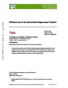
functions defined on R, which are differentiable everywhere except at 0 and concave and monotone increasing on [0, +∞) and gp (0) = 0. In particular, we will consider the following three surrogate functions: p 1) gp (x) = |x| , 0 < p ≤ 1 2) gp (x) = log(1 + |x| /p)/log(1 + 1/p), p > 0 3) gp (x) = 1 − e−|x|/p , p > 0. The first is the p-norm-like measure (with p ≤ 1) used in [15], [16], which is shown to perform well in promoting sparse solutions for compressed sensing problems. The second is the penalty function used in [11] for sparse generalized eigenvalue problem and when used to replace the ℓ1 -norm in basis pursuit, it leads to the well known iteratively reweighted ℓ1 -norm minimization algorithm [17]. The last surrogate function is used in [18] for feature selection problems, which is different from the first two surrogate functions in the sense that it has the additional property of being a lower bound of the function sgn(|x|). To provide an intuitive idea about how these surrogate functions look like, they are plotted in Fig. 1 for fixed p = 0.2. 1.4

maximize n x∈C

subject to

xH Ax − ρ kxk0

xH Bx = 1,

where the ℓ0 -norm can still be written as kxk0 = Pn i=1 sgn(|xi |), but with |xi | being the modulus of xi now. Notice that the three surrogate functions gp (x) used to approximate sgn(|x|) are all functions of |x|, by taking |x| as the modulus of a complex number, the surrogate functions are directly applicable to the complex case. The quadratic minorization function that will be described in Section III can also be constructed similarly in the complex case and at each iteration of the resulting algorithm we still need to solve a regular generalized eigenvalue problem but with complexvalued matrices. III. S PARSE G ENERALIZED E IGENVALUE P ROBLEM MM S CHEME

VIA

A. The MM method

1.2

1

p

g (x)

0.8

0.6

0.4 |x|p log(1+|x|/p)/log(1+1/p) 1−exp(−|x|/p)

0.2

0 −2

In this approach, the cardinality is considered for the real and imaginary part of the vector x separately. A more natural approach is to consider directly the complex-valued version of the ℓ0 -norm regularized generalized eigenvalue problem

−1.5

−1

−0.5

0 x

0.5

1

1.5

2

Figure 1. Three surrogate functions gp (x) that are used to approximate sgn(|x|), p = 0.2.

Pn By approximating kxk0 with i=1 gp (xi ), the original problem (4) is approximated by the following problem P maximize xT Ax − ρ ni=1 gp (xi ) x (5) subject to xT Bx = 1. With the approximation, the problem (5) is still a nonconvex nondifferentiable optimization problem, but it is a continuous problem now in contrast to the original problem (4). In the following section, we will concentrate on the approximate problem (5) and develop fast algorithms to solve it based on the MM (majorization-minimization or minorizationmaximization) scheme. Note that for simplicity of exposition, we focus on realvalued matrices throughout the paper. However, the techniques developed in this paper can be adapted for complex-valued matrix pair (A, B), with A being an n × n Hermitian matrix and B being an n × n Hermitian positive definite matrix. One approach is to transform the problem to a real-valued one by defining ˜ = [Re(x)T , Im(x)T ]T x     Re(A) −Im(A) Re(B) −Im(B) ˜ ˜ A= ,B= . Im(A) Re(A) Im(B) Re(B)

The MM method refers to the majorization-minimization method or the minorization-maximization method, which is a generalization of the well known expectation maximization (EM) algorithm. It is an approach to solve optimization problems that are too difficult to solve directly. The principle behind the MM method is to transform a difficult problem into a series of simple problems. Interested readers may refer to [19] and references therein for more details. Suppose we want to minimize f (x) over X ∈ Rn . Instead of minimizing the cost function f (x) directly, the MM approach optimizes a sequence of approximate objective functions that majorize f (x). More specifically, starting from a feasible point x(0) , the algorithm produces a sequence {x(k) } according to the following update rule x(k+1) ∈ arg min u(x, x(k) ),

(6)

x∈X

where x(k) is the point generated by the algorithm at iteration k, and u(x, x(k) ) is the majorization function of f (x) at x(k) . Formally, the function u(x, x(k) ) is said to majorize the function f (x) at the point x(k) provided u(x, x(k) ) ≥ f (x),

u(x(k) , x(k) ) = f (x(k) ).

∀x ∈ X ,

(7) (8)

In other words, function u(x, x(k) ) is a global upper bound for f (x) and coincides with f (x) at x(k) . It is easy to show that with this scheme, the objective value is decreased monotonically at every iteration, i.e., f (x(k+1) ) ≤ u(x(k+1) , x(k) ) ≤ u(x(k) , x(k) ) = f (x(k) ). (9) The first inequality and the third equality follow from the the properties of the majorization function, namely (7) and (8) respectively and the second inequality follows from (6). Note that with straightforward changes, similar scheme can be applied to maximization. To maximize a function f (x),

4 3.5

we need to minorize it by a surrogate function u(x, x(k) ) and maximize u(x, x(k) ) to produce the next iterate x(k+1) . A function u(x, x(k) ) is said to minorize the function f (x) at the point x(k) if −u(x, x(k) ) majorizes −f (x) at x(k) . This scheme refers to minorization-maximization and similarly it is easy to shown that with this scheme the objective value is increased at each iteration.

g (x ) p

i

u(x ,2) i

3

2.5

2

1.5

1

B. Quadratic Minorization Function Having briefly introduced the general MM framework, let us return to the approximate sparse generalized eigenvalue problem (SGEP) in (5). To apply the MM scheme, the key step is to find an appropriate minorization function for the objective of (5) at each iteration such that the resulting problem is easy to solve. To construct such a minorization function, T we keep the quadratic minorize the Pn term x Ax and onlyP penalty term −ρ i=1 gp (xi ) (i.e., majorize ρ ni=1 gp (xi )). More specifically, at iteration k we majorize each of the sur(k) rogate functions gp (xi ), i = 1, . . . , n at xi with a quadratic (k) (k) (k) (k) 2 function wi xi + ci , where the coefficients wi and ci (k) are determined by the following two conditions (for xi 6= 0): 2  (k) (k) (k) (k) (10) + ci , xi gp (xi ) = wi (k)

gp′ (xi ) =

(k) (k)

2wi xi ,

(11)

i.e., the quadratic function coincides with the surrogate func(k) (k) tion gp (xi ) at xi and is also tangent to gp (xi ) at xi . Due to the fact that the surrogate functions of interest are differentiable and concave for xi > 0 (also for xi < 0), the second condition implies that the quadratic function is a global upper bound of the surrogate gp (xi ). Then the Pfunction n objective of (5), i.e., xT Ax − ρ i=1 gp (x i ), is minorized  Pn  (k) 2 (k) T by the quadratic function x Ax − ρ i=1 wi xi + ci , which can be written more compactly as n   X (k) (12) ci , xT A − ρDiag(w(k) ) x − ρ i=1

where w(k) =

(k) (k) [w1 , . . . , wn ]T .

0.5

0 −5

−4

−3

−2

−1

0 x

1

2

3

4

5

i

Figure 2. The function gp (xi ) = |xi |p with p = 0.5 and its quadratic (k) majorization function at xi = 2.

deviations curve fitting problem (i.e., regression with ℓ1 -norm cost function) via iteratively solving a series of weighted least squares problems and the resulting algorithm is known as the iteratively reweighted least squares (IRLS) algorithm [12]. Later the idea was applied in signal processing for sparse signal reconstruction in [15], [21]. Recently, the IRLS approach has also been applied in Compressed Sensing [16]. Algorithms based on this idea often have the infamous singularity issue (k) (k) [13], that is, the quadratic majorization function wi x2i + ci (k) is not defined at xi = 0, due to the nondifferentiability of gp (xi ) at xi = 0. For example, considering the quadratic p majorization function of gp (xi ) = |xi | , 0 < p ≤ 1 in (15), (k) p−2 it is easy to see that the coefficient p2 xi is not defined (k)

at xi = 0. To tackle this problem, the authors of [13] proposed to define the majorization function at the particular (k) point xi = 0 as ( +∞, xi 6= 0 u(xi , 0) = 0, xi = 0, (k)

(k) (k) function wi x2i + ci p gp (xi ) = |xi | , 0
0, for example, for the p quadratic majorization function of gp (x i ) = |xi | , 0 < p ≤ 1 p−2 (k) by in (15), replace the coefficient p2 xi (k) wi

p = 2

 p−2  2 2 (k) +ǫ xi ,

which is the so called damping approach used in [16]. A potential problem of this approach is that although ǫ is small, we have no idea how it will affect the convergence of the algorithm, since the corresponding quadratic function is no longer a majorization function of the surrogate function.

5

C. Smooth Approximations of Non-differentiable Surrogate Functions To tackle the singularity issue arised during the construction of the quadratic minorization function in (12), in this subsection we propose to incorporate a small ǫ > 0 in a more systematic way. The idea is to approximate the non-differentiable surrogate function gp (x) with a differentiable function of the following form ( ax2 , |x| ≤ ǫ ǫ gp (x) = gp (x) − b, |x| > ǫ, which aims at smoothening the non-differentiable surrogate function around zero by a quadratic function. To make the function gpǫ (x) continuous and differentiable at x = ±ǫ, the following two conditions are needed aǫ2 = gp (ǫ) − b, 2aǫ = g′ (ǫ) g′ (ǫ) gp′ (ǫ), which lead to a = p2ǫ , b = gp (ǫ) − p2 ǫ. Thus, the smooth approximation of the surrogate function that will be employed is ( g′ (ǫ) p 2 |x| ≤ ǫ 2ǫ x , (16) gpǫ (x) = gp′ (ǫ) gp (x) − gp (ǫ) + 2 ǫ, |x| > ǫ, where ǫ > 0 is a constant parameter. Example 2. The smooth approximation of the function gp (x) = |x|p , 0 < p ≤ 1 is ( p p−2 2 ǫ x , |x| ≤ ǫ ǫ gp (x) = 2 p (17) |x| − (1 − p2 )ǫp , |x| > ǫ. The case with p = 0.5 and ǫ = 0.05 is illustrated in Fig. 3. When p = 1, the smooth approximation (17) is the well known Huber penalty function and the application of Huber penalty as smoothed absolute value has been used in [22] to derive fast algorithms for sparse recovery. 1 0.9 0.8 0.7 0.6 0.5 0.4 0.3 0.2

g (x)

0.1

gp(x)

0 −1

p ε

−0.5

0 x

0.5

1

Figure 3. The function gp (x) = |x|p with p = 0.5 and its smooth approximation gpǫ (x) with ǫ = 0.05.

With this smooth approximation, the problem (5) becomes the following smoothed one: Pn maximize xT Ax − ρ i=1 gpǫ (xi ) x (18) subject to xT Bx = 1, where gpǫ (·) is the function given by (16). We now majorize the smoothed surrogate functions gpǫ (xi ) with quadratic functions

and the coefficients of the quadratic majorization functions are (k) summarized in Table I (we have omitted the coefficient ci since it is irrelevant for the MM algorithm). Notice that the (k) (k) quadratic functions wi x2i + ci are now well defined. Thus, the smooth approximation we have constructed can be viewed as a systematic way to incorporate a small ǫ > 0 to deal with the singularity issue of IRLS type algorithms. Although there is no singularity issue when applying the quadratic minorization to the smoothed problem (18), a natural question is if we solve the smoothed problem, what can we say about the solution with regard to the original problem (5). In the following, we present some results which aim at answering the question. Lemma 3. Let gp (·) be a continuous even function defined on R, differentiable everywhere except at zero, concave and monotone increasing on [0, +∞) with gp (0) = 0. Then the smooth approximation gpǫ (x) defined by (16) is a global lower bound of gp (x) and gpǫ (x) + gp (ǫ) − bound of gp (x).

gp′ (ǫ) 2 ǫ

is a global upper

Proof: The lemma is quite intuitive and the proof is omitted for lack of space. Proposition 4. Let f (x) be the objective of the problem (5), with gp (·) as in Lemma 3 and fǫ (x) be the objective of the smoothed problem (18) with gpǫ (·) as in (16). Let x⋆ be the optimal solution of the problem (5) and x⋆ǫ be the optimal solu⋆ ⋆ tionof the smoothed )−f  problem (18). Then  0 ≤ f (x  (xǫ ) ≤ gp′ (ǫ) gp′ (ǫ) ρn gp (ǫ) − 2 ǫ and limǫ↓0 ρn gp (ǫ) − 2 ǫ = 0.

Proof: See Appendix A. Proposition 4 gives a suboptimality bound on the solution of the smoothed problem (18) in the sense that we can solve the original problem (5) to a very high accuracy by solving the smoothed problem (18) with a small enough ǫ (say ǫ ≤ 10−6 , and ǫ = 10−8 is used in our simulations). Of course, in general it is hard to solve either problem (5) or (18) to global maximum or even local maximum, since both of them are nonconvex. But from this point, there may be advantages in solving the smoothed problem with the smoothing parameter ǫ decreasing gradually, since choosing a relatively large ǫ at the beginning can probably smoothen out some undesirable local maxima, so that the algorithm can escape from these local points. This idea has been used with some success in [16], [22]. A decreasing scheme of ǫ will be considered later in the numerical simulations. D. Iteratively Reweighted Quadratic Minorization

With the quadratic minorization function constructed and the smoothing technique used to deal with the singularity issue, we are now ready to state the overall algorithm for the approximate SGEP in (5). First, we approximate the non-differentiable surrogate functions gp (xi ) by smooth functions gpǫ (xi ), which leads to the smoothed problem (18). Then at iteration k, we construct
the quadratic minorization function xT A − ρDiag(w(k) ) x − Pn (k) ρ i=1 ci of the objective via majorizing each smoothed

6

Table I S MOOTH APPROXIMATION gpǫ (xi ) OF THE SURROGATE FUNCTIONS gp (xi ) AND THE QUADRATIC MAJORIZATION FUNCTIONS (k) (k) (k) (k) u(xi , xi ) = wi x2i + ci AT xi . (k)

Smooth approximation gpǫ (xi ) ( p p−2 2 ǫ xi , |xi | ≤ ǫ 2 |xi |p − (1 − p2 )ǫp , |xi | > ǫ

Surrogate function gp (xi ) |xi |p , 0 < p ≤ 1

log(1 + |xi | /p)/ log(1 + 1/p), p > 0

  

x2 i , 2ǫ(p+ǫ) log(1+1/p) ǫ log(1+|xi |/p)−log(1+ǫ/p)+ 2(p+ǫ)

  e−ǫ/p x2 ,

log(1+1/p)

i 2pǫ  −e−|xi |/p + 1 +

1 − e−|xi |/p , p > 0

|xi | ≤ ǫ , |xi | > ǫ |xi | ≤ ǫ

ǫ 2p

(k)

surrogate function gpǫ (xi ) at xi by a quadratic function (k) (k) wi x2i +ci and solve the following minorized problem (with the constant term ignored)
maximize xT A − ρDiag(w(k) ) x x (19) subject to xT Bx = 1, which is to find the leading generalized eigenvector of the matrix pair (A − ρDiag(w(k) ), B), where w(k) = (k) (k) (k) [w1 , . . . , wn ]T and wi , i = 1, . . . , n are given in Table I. The method is summarized in Algorithm 1 and we will refer to it as IRQM (Iterative Reweighed Quadratic Minorization), since it is based on iteratively minorizing the penalty function with reweighted quadratic function. Algorithm 1 IRQM - Iteratively Reweighed Quadratic Minorization algorithm for the sparse generalized eigenvalue problem (5). Require: A ∈ Sn , B ∈ Sn++ , ρ > 0, ǫ > 0 1: Set k = 0, choose x(0) ∈ {x : xT Bx = 1} 2: repeat 3: Compute w(k) according to Table I. 4: x(k+1) ←leading generalized eigenvector of the matrix pair (A − ρDiag(w(k) ), B) 5: k ←k+1 6: until convergence 7: return x(k) At every iteration of the proposed IRQM algorithm, we need to find the generalized eigenvector of the matrix pair (A−ρDiag(w(k) ), B) corresponding to the largest generalized eigenvalue. Since B ∈ Sn++ , a standard approach for this problem is to transform it to a standard eigenvalue problem via the Cholesky decomposition of B. Then standard algorithms, such as power iterations (applied to a shifted matrix) and Lanczos method can be used. The drawback of this approach is that a matrix factorization is needed, making it less attractive (k) when this factorization is expensive. Besides, as some wi become very large, the problem is highly ill-conditioned and standard iterative algorithms may suffer from extremely slow convergence. To overcome these difficulties, we provide a preconditioned steepest ascent method, which is matrix factorization free and employes preconditioning to deal with the ill-conditioning



wi   p ǫp−2 , 2 p−2  p x(k) , i 2

 1  2ǫ(p+ǫ) log(1+1/p) , 

(k) x ≤ ǫ i (k) x > ǫ i (k) x ≤ ǫ i (k) , x >ǫ

1 (k) (k) 2 log(1+1/p) xi ( xi +p)

 −ǫ/p e  ,  2pǫ (k) /p − x i e  (k) ,  2p x

e−ǫ/p , |xi | > ǫ

i

i

(k) x ≤ ǫ i (k) x > ǫ i

problem. Let us derive the steepest ascent method without preconditioning first. The key step is to reformulate the leading generalized eigenvalue problem as maximizing the Rayleigh quotient ˜ xT Ax (20) R(x) = T x Bx ˜ = A − ρDiag(w(k) ). Let over the domain x 6= 0, where A (l) x be the current iterate, the gradient of R(x) at x(l) is   2 ˜ (l) − R(x(l) )Bx(l) , Ax x(l)T Bx(l) ˜ (l) − which is an ascent direction of R(x) at x(l) . Let r(l) = Ax (l) (l) R(x )Bx , the steepest ascent method searches along the line x(l) + τ r(l) for a τ that maximizes the Rayleigh quotient R(x(l) + τ r(l) ). Since the Rayleigh quotient R(x(l) + τ r(l) ) is a scalar function of τ , the maximum will be achieved either at points with zero derivative or as τ goes to infinity. Setting the derivative of R(x(l) + τ r(l) ) with respect to τ equal to 0, we can get the following quadratic equation aτ 2 + bτ + c = 0,

(21)

where a b c

˜ (l) x(l)T Br(l) − r(l)T Br(l) x(l)T Ar ˜ (l) = r(l)T Ar ˜ (l) x(l)T Bx(l) − r(l)T Br(l) x(l)T Ax ˜ (l) = r(l)T Ar ˜ (l) x(l)T Bx(l) − r(l)T Bx(l) x(l)T Ax ˜ (l) . = r(l)T Ax

Let us denote Bxx = x(l)T Bx(l) , Brr = r(l)T Br(l) and Bxr = x(l)T Br(l) , by direct computation we have 

2 2


b2 − 4ac = Bxx Brr R(r(l) ) − R(x(l) ) − 2Bxr r(l) 2

4


2 + 4 r(l) Bxx Brr − Bxr . 2

According to Cauchy-Schwartz inequality, it is easy to see 2 that Bxx Brr − Bxr ≥ 0, thus b2 − 4ac ≥ 0, which implies that the equation (21) has one or two real roots. By comparing the Rayleigh quotient R(x(l) + τ r(l) ) at the roots of equation (21) with R(r(l) ) (the Rayleigh quotient corresponding to τ → ∞), we can determine the steepest ascent. It is worth noting that the coefficients of the equation (21) can be computed by matrix-vector multiplications and inner products only, thus very efficient.

7

Though the per-iteration computational complexity of this steepest ascent method is very low, it may converge very (k) slow, especially when some wi become very large. To accelerate the convergence, we introduce a preconditioner here. Preconditioning is an important technique in iterative methods for solving large system of linear equations, for example the widely used preconditioned conjugate gradient method. It can also be used for eigenvalue problems. In the steepest ascent method, to introduce a positive definite preconditioner P, we simply multiply the residual r(l) by P. The steepest ascent method with preconditioning for the leading generalized eigenvalue problem (19) is summarized in Algorithm 2. To use the algorithm in practice, the preconditioner P remains to be chosen. For the particular problem of interest, we choose a diagonal P as follows 
−1 ρkw(k) k  Diag ρw(k) + |diag(A)| , kdiag(A)k2 > 102 P= 2 In . otherwise. In other words, we apply a preconditioner only when some elements of w(k) become relatively large. Since the preconditioner P we choose here is positive definite, the direction Pr(l) is still an ascent direction and the algorithm is still monotonically increasing. For more details regarding preconditioned eigensolvers, the readers can refer to the book [23]. In practice, the preconditioned steepest ascent method usually converges to the leading generalized eigenvector, but it is not guaranteed in principle, since the Rayleigh quotient is not concave. But note that the descent property (9) of the majorization-minimization scheme depends only on decreasing u(x, x(k) ) and not on minimizing it. Similarly, for the minorization-maximization scheme used by Algorithm 1, to preserve the ascent property, we only need to increase the objective of (19) at each iteration, rather than maximizing it. Since the steepest ascent method increases the objective at every iteration, thus when it is applied (initialized with the solution of previous iteration) to compute the leading generalized eigenvector at each iteration of Algorithm 1, the ascent property of Algorithm 1 can be guaranteed.

E. Sparse GEP with Special Structure Until now we have considered the sparse GEP in the general case with A ∈ Sn , B ∈ Sn++ and derived an iterative algorithm IRQM. If we assume more properties or some special structure for A and B, then we may derive simpler and more efficient algorithms. In the following, we will consider the case where A ∈ Sn+ and B = Diag(b), b ∈ Rn++ . Notice that although this is a special case of the general sparse GEP, it still includes the sparse PCA problem as a special case where B = In . We first present two results that will be used when deriving fast algorithms for this special case. Proposition 5. Given a ∈ Rn , w, b ∈ Rn++ , ρ > 0, let Imin = arg min{ρwi /bi : i ∈ {1, . . . , n}}, µmin = − min{ρwi /bi : i ∈ {1, . . . , n}} and s = P bi a2i i∈I / min (µmin bi +ρwi )2 . Then the problem maximize x

subject to

2aT x − ρxT Diag(w)x xT Diag(b)x = 1

admits the following solution: 2 • If ∃i ∈ Imin , such that ai > 0 or s > 1, then ai , i = 1, . . . , n, x⋆i = µbi + ρwi where µ > µmin is given by the solution of the scalar equation n X bi a2i = 1. (µbi + ρwi )2 i=1 •

Otherwise,   / (µmin bi + ρwi ) , i ∈ / Imin a pi ⋆ xi = (1 − s) /bi , i = max{i : i ∈ Imin }   0, otherwise.

Proof: See Appendix B.

Proposition 6. Given a ∈ Rn with |a1 | ≥ . . . ≥ |an | and ρ > 0, then the problem maximize x

Algorithm 2 Preconditioned steepest ascent method for problem (19). n

∈ Sn++ , (0)

(k)

Require: A ∈ S , B w ,ρ>0 1: Set l = 0, choose x ∈ {x : xT Bx = 1} ˜ = A − ρDiag(w(k) ) 2: Let A 3: repeat ˜ (l) /x(l)T Bx(l) 4: R(x(l) ) = x(l)T Ax (l) (l) ˜ 5: r = Ax − R(x(l) )Bx(l) 6: r(l) = Pr(l) 7: x = x(l) + τ r(l) , with τ chosen to maximize R(x(l) + τ r(l) ) √ 8: x(l+1) = x/ xT Bx 9: l =l+1 10: until convergence 11: return x(l)

(22)

aT x − ρ kxk0

subject to kxk2 = 1

admits the following solution: • If |a1 | ≤ ρ, then ( sgn(a1 ), i = 1 ⋆ xi = 0, otherwise. •

(23)

(24)

Otherwise, x⋆i =

( qPs 2 ai / j=1 aj , i ≤ s 0,

otherwise,

where s is the largest integer p that satisfies the following inequality q qP Pp−1 2 p 2 > (25) a i=1 ai + ρ. i=1 i

Proof: See Appendix C.

8

Let us return to the problem. In this special case, the smoothed problem (18) reduces to Pn maximize xT Ax − ρ i=1 gpǫ (xi ) x (26) subject to xT Diag(b)x = 1. The previously derived IRQM algorithm can be used here, but in that iterative algorithm, we need to find the leading generalized eigenvector at each iteration, for which another iterative algorithm is needed. By exploiting the special structure of this case, in the following we derive a simpler algorithm that at each iteration has a closed-form solution. Notice that, in this case, A ∈ Sn+ , the first term xT Ax in the objective is convex and can be minorized by its tangent plane 2xT Ax(k) at x(k) . So instead of only minorizing the second term, we can minorize both terms. This suggests solving the following minorized problem at iteration k: maximize x

subject to

2xT Ax(k) − ρxT Diag(w(k) )x

(27)

xT Diag(b)x = 1,

where x(k) is the solution at iteration k and w(k) is computed according to Table I. The problem is a nonconvex QCQP, but by letting a = Ax(k) and w = w(k) , we know from Proposition 5 that it can be solved in closed-form. The iterative algorithm for solving problem (26) is summarized in Algorithm 3. Algorithm 3 The MM algorithm for problem (26). Require: A ∈ Sn+ , b ∈ Rn++ , ρ > 0, ǫ > 0 1: Set k = 0, choose x(0) ∈ {x : xT Diag(b)x = 1} 2: repeat 3: a = Ax(k) 4: Compute w(k) according to Table I. 5: Solve the following problem according to Proposition 5 and set the solution as x(k+1) : max{2aT x − ρxT Diag(w(k) )x : xT Diag(b)x = 1} x

6: 7: 8:

k =k+1 until convergence return x(k)

x

xT Ax − ρ kxk0

(28)

subject to xT Diag(b)x = 1. 1

˜ = Diag(b) 2 x and First, we define a new variable x

− 12 ˜ xk0 , the problem can be using the fact Diag(b) x = k˜ 0 rewritten as ˜ x − ρ k˜ ˜ T A˜ maximize x xk0 ˜ x (29) T ˜ x ˜ = 1, subject to x ˜ = Diag(b)− 2 ADiag(b)− 2 . where A Now the idea is to minorize only the quadratic term by ˜ (k) at its tangent plane, while keeping the ℓ0 -norm. Given x 1

maximize ˜ x

1

˜ x(k) − ρ k˜ 2˜ xT A˜ xk0

subject to k˜ xk2 = 1,

(30)

which has a closed-form solution. To see this, we first define ˜ x(k) and sort the entries of vector a according to a = 2A˜ the absolute value (only needed for entries with |ai | > ρ) in descending order, then Proposition 6 can be readily applied to obtain the solution. Finally we need to reorder the solution back to the original ordering. This algorithm for solving problem (28) is summarized in Algorithm 4. It is worth noting that although the derivations of Algorithms 3 and 4 require A to be symmetric positive semidefinite, the algorithms can also be used to deal with the more general case A ∈ Sn . When the matrix A in problem (26) or (28) is not positive semidefinite, we can replace A with Aα = A + αDiag(b), with α ≥ −λmin (A)/bmin such that Aα ∈ Sn+ , where λmin (A) is the smallest eigenvalue of matrix A and bmin is the smallest entry of b. Since the additional term αxT Diag(b)x in the objective is just a constant α over the constraint set, it is easy to see that after replacing A with Aα the resulting problem is equivalent to the original one. Then the Algorithm 3 or 4 can be readily applied. Algorithm 4 The MM algorithm for problem (28). Require: A ∈ Sn+ , b ∈ Rn++ , ρ > 0 ˜ (0) ∈ {˜ ˜T x ˜ = 1} 1: Set k = 0, choose x x:x 1 − 12 ˜ 2: Let A = Diag(b) ADiag(b)− 2 3: repeat ˜ x(k) 4: a = 2A˜ 5: Sort a with the absolute value in descending order. ˜ (k+1) according to Proposition 6: 6: Compute x ˜ (k+1) ∈ arg max{aT x ˜ − ρ k˜ x xk0 : k˜ xk2 = 1} x ˜

7: 8: 9: 10:

In fact, in this special case, we can apply the MM scheme to solve the original problem (4) directly, without approximating kxk0 , i.e., solving maximize

iteration k, linearizing the quadratic term yields

˜ (k+1) Reorder x k =k+1 until convergence 1 ˜ (k) return x = Diag(b)− 2 x

IV. C ONVERGENCE

ANALYSIS

The algorithms proposed in this paper are all based on the minorization-maximization scheme, thus according to subsection III-A, we know that the sequence of objective values evaluated at {x(k) } generated by the algorithms is nondecreasing. Since the constraint sets in our problems are compact, the sequence of objective values is bounded. Thus, the sequence of objective values is guaranteed to converge to a finite value. The monotonicity makes MM algorithms very stable. In this section, we will analyze the convergence property of the sequence {x(k) } generated by the algorithms. Let us consider the IRQM algorithm in Algorithm 1, in which the minorization-maximization scheme is applied to the smoothed problem (18). In the problem, the objective is neither convex nor concave and the constraint set is also nonconvex. But as we shall see later, after introducing a

9

technical assumption on the surrogate function gp (x), the problem is equivalent to a problem which maximizes a convex function over a convex set and we will prove that the sequence generated by the IRQM algorithm converges to the stationary point of the equivalent problem. The convergence of the Algorithm 3 can be proved similarly, since the minorization function applied can also be convexified. First, let us give the assumption and present some results that will be useful later. Assumption 1. The surrogate function gp (x) is twice differentiable on (0, +∞) and its gradient gp′ (x) is convex on (0, +∞). It is easy to verify that the three surrogate functions listed in Table (I) all satisfy this assumption. With this assumption, the first result shows that the smooth approximation gpǫ (x) we have constructed is Lipschitz continuously differentiable. Lemma 7. Let gp (·) be a continuous even function defined on R, differentiable everywhere except at zero, concave and monotone increasing on [0, +∞) with gp (0) = 0. Let Assumption 1 be satisfied. Then the smooth approximation gpǫ (x) defined by (16) is Lipschitz continuously differentiable with g′ (ǫ) Lipschitz constant L = max{ pǫ , gp′′ (ǫ) }.

Proof: See Appendix D. Next, we recall a useful property of Lipschitz continuously differentiable functions [24].

Proposition 10. Let f : Rn → R be a convex function. Let S ∈ Rn be an arbitrary set and conv(S) be its convex hull. Then sup{f (x)|x ∈ conv(S)} = sup{f (x)|x ∈ S}, where the first supremum is attained only when the second (more restrictive) supremum is attained. According to Proposition 10, we can further relax the constraint xT Bx = 1 in problem (31) to xT Bx ≤ 1, namely, the problem P maximize xT (A + αB) x − ρ ni=1 gpǫ (xi ) x (32) subject to xT Bx ≤ 1 is still equivalent to problem (18) in the sense that they admit the same set of optimal solutions. Let us denote the objective function of problem (32) by fǫα (x) and define B = {x ∈ Rn |xT Bx ≤ 1}, then a point x⋆ is referred to as a stationary point of problem (32) if ∇fǫα (x⋆ )T (x − x⋆ ) ≤ 0,

∀x ∈ B.

(33)

Theorem 11. Let {x(k) } be the sequence generated by the IRQM algorithm in Algorithm 1. Then every limit point of the sequence {x(k) } is a stationary point of the problem (32), which is equivalent1 to the problem (18).

Proposition 8. If f : Rn → R is Lipschitz continuously differentiable on a convex set C with some Lipschitz constant L, then ϕ(x) = f (x) + α2 xT x is a convex function on C for every α ≥ L.

Proof: Denote the objective function of the problem (18) by fǫ (x) and its quadratic minorization function
at x(k) by q(x|x(k) ), i.e., q(x|x(k) ) = xT A − ρDiag(w(k) ) x. Denote S = {x ∈ Rn |xT Bx = 1} and B = {x ∈ Rn |xT Bx ≤ 1}. According to the general MM framework, we have

The next result then follows, showing that the smoothed problem (18) is equivalent to a problem in the form of maximizing a convex function over a compact set.

fǫ (x(k+1) ) ≥ q(x(k+1) |x(k) ) ≥ q(x(k) |x(k) ) = fǫ (x(k) ),

Lemma There exists α > 0 such that xT (A + αB) x − Pn 9. ǫ ρ i=1 gp (xi ) is convex and the problem Pn maximize xT (A + αB) x − ρ i=1 gpǫ (xi ) x (31) subject to xT Bx = 1 is equivalent to the problem (18) in the sense that they admit the same set of optimal solutions. From Lemma 7, it is easy to see that xT Ax − PnProof: ǫ ρ i=1 gp (xi ) is Lipschitz continuously differentiable. Assume the Lipschitz constant of
its gradient P is L, then according to Proposition 8, xT A + L2 I x − ρ ni=1 gpǫ (xi ) is convex. Since B is positive definite, λmin (B) > 0. By choosing L L T α ≥ 2λmin (B) , we have that x (αB − 2 I)x is convex. T The Pnsum ǫof the two convex functions, i.e., x (A + αB) x − ρ i=1 gp (xi ), is convex. Since the additional term αxT Bx is just a constant α over the constraint set xT Bx = 1, it is obvious that any solution of problem (31) is also a solution of problem (18) and vice versa. Generally speaking, maximizing a convex function over a compact set remains a hard nonconvex problem. There is some consolation, however, according to the following result in convex analysis [25].

which means {fǫ (x(k) )} is a non-decreasing sequence. Assume that there exists a converging subsequence x(kj ) → ∞ x , then q(x(kj+1 ) |x(kj+1 ) ) = fǫ (x(kj+1 ) ) ≥ fǫ (x(kj +1) )

≥ q(x(kj +1) |x(kj ) ) ≥ q(x|x(kj ) ), ∀x ∈ S.

Letting j → +∞, we obtain q(x∞ |x∞ ) ≥ q(x|x∞ ), ∀x ∈ S. It is easy to see that we can always find α > 0 such that qα (x|x∞ ) = q(x|x∞ ) + αxT Bx is convex and x∞ is still a global maximizer of qα (x|x∞ ) over S. Due to Lemma 9, we can always choose α large enough such that fǫα (x) = fǫ (x) + αxT Bx is also convex. By Proposition 10, we have qα (x∞ |x∞ ) ≥ qα (x|x∞ ), ∀x ∈ B, i.e., x∞ is a global maximizer of qα (x|x∞ ) over the convex set B. As a necessary condition, we get ∇qα (x∞ |x∞ )T (x − x∞ ) ≤ 0, ∀x ∈ B. 1 The equivalence of the problem (32) and (18) is in the sense that they have the same set of optimal solutions, but they may have different stationary points. The convergence to a stationary point of problem (32) does not imply the convergence to a stationary point of problem (18).

10

Since ∇fǫα (x∞ ) = ∇qα (x∞ |x∞ ) by construction, we obtain ∇fǫα (x∞ )T (x

∞

− x ) ≤ 0, ∀x ∈ B,

implying that x∞ is a stationary point of the problem (32), which is equivalent to the problem (18) according to Lemma 9 and Proposition 10. We note that in the above convergence analysis of Algorithm 1, the leading generalized eigenvector is assumed to be computed exactly at each iteration. Recall that the Algorithm 2 is not guaranteed to converge to the leading generalized eigenvector in principle, so if it is applied to compute the leading generalized eigenvector, the convergence of Algorithm 1 to a stationary point is no longer guaranteed. V. N UMERICAL E XPERIMENTS To compare the performance of the proposed algorithms with existing ones on the sparse generalized eigenvalue problem (SGEP) and some of its special cases, we present some experimental results in this section. All experiments were performed on a PC with a 3.20GHz i5-3470 CPU and 8GB RAM.

distributed and following N (0, 1). For both algorithms, the initial point x(0) is chosen randomly with each entry following
T N (0, 1) and then normalized such that x(0) Bx(0) = 1. The parameter p of the surrogate function is chosen to be 1 and the regularization parameter is ρ = 0.1. The computational time for problems with different sizes are shown in Figure 4. The results are averaged over 100 independent trials. From Figure 4, we can see that the preconditioning scheme is indeed important for the efficiency of Algorithm 2 and the proposed IRQM algorithm is much faster than the DC-SGEP algorithm. It is worth noting that the solver Mosek which is used to solve the QCQPs for the DC-SGEP algorithm is well known for its efficiency, while the IRQM algorithm is entirely implemented in Matlab. The lower computational complexity of the IRQM algorithm, compared with the DC-SGEP algorithm, attributes to both the lower per iteration computational complexity and the faster convergence. To show this, the evolution of the objective function for one trial with n = 100 is plotted in Figure 5 and we can see that the proposed IRQM algorithm takes much fewer iterations to converge. One may also notice that the two algorithms converge to the same objective value, but this does not hold in general since the problem is nonconvex.

A. Sparse Generalized Eigenvalue Problem

2 Mosek,

available at http://www.mosek.com/

2

10

DC−SGEP IRQM (without preconditioning) IRQM (proposed) 1

10 Average running time (s)

In this subsection, we evaluate the proposed IRQM algorithm for the sparse generalized eigenvalue problem in terms of computational complexity and the ability to extract sparse generalized eigenvectors. The benchmark method considered here is the DC-SGEP algorithm proposed in [10], [11], which is based on D.C. (difference of convex functions) programming and minorization-maximization (to the best of our knowledge, this is the only algorithm proposed for this case). The problem that DC-SGEP solves is just (5) with the surrogate function gp (x) = log(1 + |x| /p)/log(1 + 1/p), but the equality constraint xT Bx = 1 is relaxed to xT Bx ≤ 1. The DC-SGEP algorithm requires solving a convex quadratically constrained quadratic program (QCQP) at each iteration, which is solved by the solver Mosek2 in our In the condition is experiments. experiments, the stopping
f (x(k+1) ) − f (x(k) ) / max 1, f (x(k) ) ≤ 10−5 for both algorithms. For the proposed IRQM algorithm, the smoothing parameter is set to be ǫ = 10−8 . 1) Computational Complexity : In this subsection, we compare the computational complexity of the proposed IRQM Algorithm 1 with the DC-SGEP algorithm. The surrogate function gp (x) = log(1 + |x| /p)/log(1 + 1/p) is used for both algorithms in this experiment. The preconditioned steepest ascent method given in Algorithm 2 is applied to compute the leading generalized eigenvector at every iteration of the IRQM algorithm. To illustrate the effectiveness of the preconditioning scheme employed in Algorithm 2, we also consider computing the leading generalized eigenvector by invoking Algorithm 2 but without preconditioning, i.e., setting P = In . The data matrices A ∈ Sn and B ∈ Sn++ are generated as A = C+CT and B = DT D, with C ∈ Rn×n , D ∈ R1.2n×n and the entries of both C and D independent, identically

0

10

−1

10

−2

10

50

100

150 Problem size n

200

250

Figure 4. Average running time versus problem size. Each curve is an average of 100 random trials.

2) Random Data with Underlying Sparse Structure : In this section, we generate random matrices A ∈ Sn and B ∈ Sn++ such that the matrix pair (A, B) has a few sparse generalized eigenvectors. To achieve this, we synthesize the data through the generalized eigenvalue decomposition A = V−T Diag(d)V−1 and B = V−T V−1 , where the first k columns of V ∈ Rn×n are pre-specified sparse vectors and the remaining columns are generated randomly, d is the vector of the generalized eigenvalues. Here, we choose n = 100 and k = 2, where the two sparse generalized eigenvectors are specified as follows ( Vi,1 = √15 for i = 1, . . . , 5, Vi,1 = 0

otherwise,

11 3

1 IRQM−exp, p=1 IRQM−Lp, p=1 IRQM−log, p=1 DC−SGEP, p=1

0.9

2.5

0.8 Chance of exact recovery

objective value

2

1.5

1

0.5

0.7 0.6 0.5 0.4 0.3 0.2

IRQM (proposed) DC−SGEP

0

0.1 0

20

30 iterations

40

50

60

Evolution of the objective function for one trial with n = 100.

(

Vi,2 =

√1 5

Vi,2 = 0

0

1

2 3 Regularization parameter ρ

4

5

Figure 6. Chance of exact recovery versus regularization parameter ρ. Parameter p = 1 is used for the surrogate functions.

for i = 6, . . . , 10, 1

otherwise,

and the generalized eigenvalues are chosen as  d1 = 10    d = 8 2  di = 12, for i = 3, 4, 5    di ∼ N (0, 1), otherwise.

We generate 200 pairs of (A, B) as described above and employ the algorithms to compute the leading sparse generalized eigenvector x1 ∈ R100 , which is hoped to be close to V:,1 . The underlying sparse generalized eigenvector V:,1 is considered to be successfully recovered when k|x1 | − V:,1 k2 ≤ 0.01. For the proposed IRQM algorithm, all the three surrogate functions listed in Table I are considered and we call the resulting algorithms “IRQM-log”, “IRQMLp” and “IRQM-exp”, respectively. For all the algorithms, the initial point x(0) is chosen randomly. Regarding the parameter p of the surrogate function, three values, namely 1, 0.3 and 0.1, are compared. The corresponding performance along the whole path of the regularization parameter ρ is plotted in Fig. 6, 7 and 8, respectively. From Fig. 6, we can see that for the case p = 1, the best chance of exact recovery achieved by the three IRQM algorithms are very close and all higher than that achieved by the DC-SGEP algorithm. From Fig. 7 and 8, we can see that as p becomes smaller, the best chance of exact recovery achieved by IRQM-exp, IRQM-log and DC-SGEP stay almost the same as in the case p = 1 (in fact decrease a little bit when p = 0.1), but the performance of IRQM-Lp degrades a lot. This may be explained by the fact that as p becomes smaller, p the surrogate function |x| tends to the function sgn(|x|) much faster than the other two surrogate functions. So when p = 0.1 for example, it is much more pointed and makes the algorithm easily get stuck at some local point. In this sense, the log-based and exp-based surrogate functions seem to be better choices as they are not so sensitive to the choice of p.

IRQM−exp, p=0.3 IRQM−Lp, p=0.3 IRQM−log, p=0.3 DC−SGEP, p=0.3

0.9 0.8 Chance of exact recovery

Figure 5.

10

0.7 0.6 0.5 0.4 0.3 0.2 0.1 0

0

0.5

1 Regularization parameter ρ

1.5

2

Figure 7. Chance of exact recovery versus regularization parameter ρ. Parameter p = 0.3 is used for the surrogate functions.

0.9 0.8 0.7 Chance of exact recovery

0

0.6 0.5 0.4 0.3 IRQM−exp, p=0.1 IRQM−Lp, p=0.1 IRQM−log, p=0.1 DC−SGEP, p=0.1

0.2 0.1 0

0

0.2

0.4 0.6 Regularization parameter ρ

0.8

1

Figure 8. Chance of exact recovery versus regularization parameter ρ. Parameter p = 0.1 is used for the surrogate functions.

12

3) Decreasing Scheme of the Smoothing Parameter ǫ: As have been discussed in the end of Section III-C, choosing a relatively large smoothing parameter ǫ at the beginning and decreasing it gradually may probably lead to better performance than the fixed ǫ scheme. In this section, we consider such a decreasing scheme and compare its performance with the fixed ǫ scheme in which the smoothing parameter is fixed to be ǫ = 10−8 . The decreasing scheme that we will adopt is inspired by the continuation approach in [22]. The idea is to apply the IRQM algorithm to a succession of problems with decreasing smoothing parameters ǫ(0) > ǫ(1) > · · · > ǫ(T ) and solve the intermediate problems with less accuracy, where T is the number of decreasing steps. More specifically, at step t = 0, . . . , T , we apply the IRQM (t) with smoothing parameter √ criterion algorithm ǫ and
stopping f (x(k+1) ) − f (x(k) ) / max 1, f (x(k) ) ≤ ǫ(t) /10 and then decrease the smoothing parameter for the next step by ǫ(t+1) = γǫ(t) with γ = (ǫ(T ) /ǫ(0) )1/T . At each step the IRQM algorithm is initialized with the solution of the previous step. The initial smoothing parameter is chosen as ǫ(0) = x(0) ∞ /4, where x(0) is the random initial point and the minimum smoothing parameter is set as ǫ(T ) = 10−8 , which is the parameter used in the fixed ǫ scheme. The number of decreasing steps is set to T = 5 in our experiment. The remaining settings are the same as in the previous subsection and the log-based surrogate function with parameter p = 0.3 is used for the IRQM algorithm. The performance of the two schemes are shown in Fig. 9. From the figure, we can see that the decreasing scheme of the smoothing parameter achieves a higher chance of exact recovery. 1 0.9

Chance of exact recovery

0.8 0.7 0.6 0.5 0.4 0.3 0.2 IRQM−log, decreasing ε IRQM−log, fixed ε

0.1 0

0

0.5

1 Regularization parameter ρ

1.5

2

Figure 9. Chance of exact recovery versus regularization parameter ρ. The log-based surrogate function with parameter p = 0.3 is used.

B. Sparse Principal Component Analysis (B = In ) In this section, we consider the special case of the sparse generalized eigenvalue problem in which the matrix B is the identity matrix, i.e., the sparse PCA problem, which has received most of the recent attention in the literature. In this case, the matrix A is usually a (scaled) covariance matrix. Although there exists a vast literature on sparse PCA, most

popular algorithms are essentially variations of the generalized power method (GPower) proposed in [7]. Thus we choose the GPower methods, namely GPowerℓ1 and GPowerℓ0 , as the benchmarks in this section. The Matlab code of the GPower algorithms was downloaded from the authors’ website. For the proposed Algorithm 3, the surrogate function is chosen to be gp (x) = |x| , such that the penalty function is just the ℓ1 -norm, which is the same as in GPowerℓ1 . We call the resulting algorithm ”MMℓ1 ” and the Algorithm 4 is referred to as ”MMℓ0 ” in this section. Note that for GPower methods, direct access to the original data matrix C is required. When only the covariance matrix is available, a factorization of the form A = CT C is needed (e.g., by eigenvalue decomposition or by Cholesky decomposition). If the data matrix C is of size m × n, then the per-iteration computational cost is O(mn) for all the four algorithms under consideration. 1) Computational Complexity: In this subsection, we compare the computational complexity of the four algorithms mentioned above, i.e., GPowerℓ1 , GPowerℓ0 , MMℓ1 and MMℓ0 . The data matrix C ∈ Rn×n is generated randomly with the entries independent, identically distributed and following N (0, 1). condition is set to be The stopping
f (x(k+1) ) − f (x(k) ) / max 1, f (x(k) ) ≤ 10−5 for all the algorithms. The smoothing parameter for algorithm MMℓ1 is fixed to be ǫ = 10−8 . The regularization parameter ρ is chosen such that the solutions of the four algorithms exhibit similar cardinalities (with about 5% nonzero entries). The average running time over 100 independent trials for problems with different sizes are shown in Figure 10. From the figure, we can see that the two ℓ0 -norm penalized methods are faster than the two ℓ1 -norm penalized methods and the proposed MMℓ0 is the fastest among the four algorithms, especially for problems of large size. For the two ℓ1 -norm penalized methods, the proposed MMℓ1 is slower than GPowerℓ1 , which may result from the fact that MMℓ1 minorizes both the quadratic term and the ℓ1 penalty term while GPowerℓ1 keeps the ℓ1 penalty term. It is worth noting that the GPowerℓ1 is specialized for ℓ1 penalty, while Algorithm 3 can also deal with various surrogate functions other than the ℓ1 penalty. 2) Random Data Drawn from a Sparse PCA Model: In this subsection, we follow the procedure in [6] to generate random data with a covariance matrix having sparse eigenvectors. To achieve this, we first construct a covariance matrix through the eigenvalue decomposition A = VDiag(d)VT , where the first k columns of V ∈ Rn×n are pre-specified sparse orthonormal vectors. A data matrix C ∈ Rm×n is then generated by drawing m samples from a zero-mean normal distribution with covariance matrix A, that is, C ∼ N (0, A). Following the settings in [7], we choose n = 500, k = 2, and m = 50, where the two orthonormal eigenvectors are specified as follows ( Vi,1 = √110 for i = 1, . . . , 10, Vi,1 = 0

(

Vi,2 =

√1 10

Vi,2 = 0

otherwise,

for

i = 11, . . . , 20,

otherwise.

13 0

Average running time (s)

MM−L1 (proposed) GPower−L1 GPower−L0 MM−L0 (proposed) −1

10

−2

10

−3

10

200

300

400

500 600 700 Problem size n

800

900

1000

Figure 10. Average running time versus problem size. Each curve is an average of 100 random trials.

The eigenvalues are fixed at d1 = 400, d2 = 300 and di = 1, for i = 3, . . . , 500. We randomly generate 500 data matrices C ∈ Rm×n and employ the four algorithms to compute the leading sparse eigenvector x1 ∈ R500 , which is hoped to recover V:,1 . We consider the underlying sparse eigenvector V:,1 is successfully recovered when xT1 V:,1 > 0.99. The chance of successful recovery over a wide range of regularization parameter ρ is plotted in Figure 11. The horizontal axis shows the normalized regularization parameter, that is ρ/ maxi kC:,i k2 for and MMℓ0 . For GPowerℓ1 and ρ/ maxi kC:,ik22 for GPower

ℓ0 MMℓ1 algorithm, we use ρ/ 2 CT C ∞,2 , where k·k∞,2 is the operator norm induced by k·k∞ and k·k2 . From the figure, we can see that the highest chance of exact recovery achieved by the four algorithms is the same and for all algorithms it is achieved over a relatively wide range of ρ. 0.9

biological questions. But the amount of data created in an experiment is usually large and this makes the interpretation of these data challenging. PCA has been applied as a tool in the studies of gene expression data and their interpretation [26]. Naturally, sparse PCA, which extracts principal components with only a few nonzero elements can potentially enhance the interpretation. In this subsection, we test the performance of the algorithms on gene expression data collected in the breast cancer study by Bild et al. [27]. The data set contains 158 samples over 12625 genes, resulting in a 158 × 12625 data matrix. Figure 12 shows the explained variance versus cardinality for five algorithms, including the simple thresholding scheme. The proportion of explained variance is computed as xTSPCA (CT C)xSPCA /xTPCA (CT C)xPCA , where xSPCA is the sparse eigenvector extracted by sparse PCA algorithms, xPCA is the true leading eigenvector and C is the data matrix. The simple thresholding scheme first computes the regular principal component xPCA and then keeps a required number of entries with largest absolute values. From the figure, we can see that the proportion of variance being explained increases as the cardinality increases as expected. For a fixed cardinality, the two GPower algorithms and the two proposed MM algorithms can explain almost the same amount of variance, all higher than the simple thresholding scheme, especially when the cardinality is small. 1 0.9 Proportion of explained variance

10

0.8 0.7 0.6 0.5 GPower−L1 GPower−L0 MM−L1 (proposed) MM−L0 (proposed) Simple Thresholding

0.4

0.8

0.3

Chance of exact recovery

0.7

0.2 0.6

0

500

1000 Cardinality

1500

2000

0.5

Figure 12.

Trade-off curves between explained variance and cardinality.

0.4 0.3

VI. C ONCLUSIONS

0.2

GPower−L1 GPower−L0 MM−L1 (proposed) MM−L0 (proposed)

0.1 0

0

Figure 11. parameter.

0.1

0.2

0.3 0.4 0.5 0.6 0.7 Normalized regularization parameter

0.8

0.9

1

Chance of exact recovery versus normalized regularization

3) Gene Expression Data : DNA microarrays allow measuring the expression level of thousands of genes at the same time and this opens the possibility to answer some complex

We have developed an efficient algorithm IRQM that allows to obtain sparse generalized eigenvectors of a matrix pair. After approximating the ℓ0 -norm penalty by some nonconvex surrogate functions, the minorization-maximization scheme is applied and the sparse generalized eigenvalue problem is turned into a sequence of regular generalized eigenvalue problems. The convergence to a stationary point is proved. Numerical experiments show that the proposed IRQM algorithm outperforms an existing algorithm based on D.C. programming in terms of both computational cost and support recovery. For sparse generalized eigenvalue problems with special structure

14

(but still including sparse PCA as a special instance), two more efficient algorithms that have a closed-form solution at every iteration are derived again based on the minorizationmaximization scheme. On both synthetic random data and real-life gene expression data, the two algorithms are shown experimentally to have similar performance to the state-of-theart. A PPENDIX A P ROOF OF P ROPOSITION 4 Proof: From Lemma 3, it is easy to show that   gp′ (ǫ) fǫ (x) ≥ f (x) ≥ fǫ (x) − ρn gp (ǫ) − ǫ , ∀x ∈ Rn . 2 (34) Since problems (5) and (18) have the same constraint set, we have fǫ (x⋆ǫ ) ≥ f (x⋆ ). (35)

From the fact that x⋆ is a global maximizer of problem (5), we know f (x⋆ ) ≥ f (x⋆ǫ ). (36) Combining (34), (35) and (36), yields   gp′ (ǫ) fǫ (x⋆ǫ ) ≥ f (x⋆ ) ≥ f (x⋆ǫ ) ≥ fǫ (x⋆ǫ ) − ρn gp (ǫ) − ǫ . 2 Thus, ⋆

0 ≤ f (x ) −

f (x⋆ǫ )

  gp′ (ǫ) ǫ . ≤ ρn gp (ǫ) − 2

Since gp (·) is concave and monotone increasing on [0, +∞), it is easy to show that gp (ǫ) ≥ gp′ (ǫ)ǫ ≥ 0, for any ǫ > 0. Hence gp′ (ǫ) gp (ǫ) ≥ gp (ǫ) − ǫ ≥ 0. (37) 2 Since gp (·) is continuous and monotone increasing on [0, +∞) and gp (0) = 0, we have limǫ↓0 gp (ǫ) = 0. Together with (37), we can conclude that   gp′ (ǫ) lim gp (ǫ) − ǫ = 0. ǫ↓0 2 Since ρ and n are constants, the proof is complete.

Then the third optimality condition (40) is just µ ≥ µmin , since wi > 0, ρ > 0, bi > 0. Let us consider the optimality condition in two different cases: 1) µ > µmin . In this case, µDiag(b)+ρDiag(w) ≻ 0, from the first optimality condition (38) we get x = (Diag(µb + ρw))−1 a.

Substituting it into the second optimality condition (39), yields X X bi a2i bi a2i + = 1, (44) (µbi + ρwi )2 (µbi + ρwi )2 i∈Imin

A PPENDIX B OF P ROPOSITION 5

Proof: First notice that the problem (22) is a nonconvex QCQP but with only one constraint, thus the strong duality holds [28], [29]. The optimality conditions for this problem are (µDiag(b) + ρDiag(w)) x xT Diag(b)x

= a = 1

(38) (39)

µDiag(b) + ρDiag(w)

 0.

(40)

Let us define Imin = arg min{ρwi /bi : i ∈ {1, . . . , n}}

(41)

µmin = − min{ρwi /bi : i ∈ {1, . . . , n}}.

(42)

and

i∈I / min

and it is easy to see that the left hand side is monotonically decreasing for µ ∈ (µmin , +∞). If ∃i ∈ Imin , such that a2i > 0, then the left hand side of (44) tends to +∞ as µ → µmin . Notice that the left hand side goes to 0 as µ → +∞, thus we are guaranteed to find a µ ∈ (µmin , +∞) satisfying equation (44). In practice, we may use bisection method to find the value of µ. If a2i = 0, ∀i ∈ Imin , there still exists a µ > µmin that satisfies equation (44) if and only if X bi a2i > 1. (45) (µmin bi + ρwi )2 i∈I / min

If (45) does not hold, it implies µ = µmin . 2) µ = µmin . In this case, we cannot compute x via equation (43) anymore. Then to obtain x, we first notice from (38) that ai , ∀i ∈ / Imin . (46) xi = µmin bi + ρwi Then, according to equation (39), for xi , i ∈ Imin , they just need to satisfy the following equation X X bi a2i . (47) bi x2i = 1 − (µmin bi + ρwi )2 i∈Imin

i∈I / min

When card(Imin ) > 1, (47) has infinite number of solutions and we may choose arbitrary one.

P ROOF

A PPENDIX C OF P ROPOSITION 6

Proof: The problem (23) can be rewritten as n  o maximize −ρs + max aT x : kxk2 = 1, kxk0 ≤ s . s∈{1,...,n}

P ROOF

(43)

x

The inner maximization has a closed-form solution ( qPs 2 ai / j=1 aj , i ≤ s x⋆i = 0 otherwise, then the problem becomes   qP s 2 . a maximize −ρs + i=1 i s∈{1,...,n}

It’s easy to see that the optimal s is the largest integer p that satisfies the following inequality q qP Pp−1 2 p 2 (48) i=1 ai > i=1 ai + ρ. By squaring both sides of this inequality, we get q Pp−1 2 a2p > ρ2 + 2ρ i=1 ai ,

15

which means |ap | > ρ is a necessary condition for (48) to be satisfied. Thus, in practice to find the largest integer p that satisfies (48) we only need to check for all p’s with |ap | > ρ. If 0 < |a1 | ≤ ρ, it is easy to see that the solution of the problem (23) is given by (24). A PPENDIX D P ROOF OF L EMMA 7 Proof: From the way gpǫ (x) is constructed, it is continuously differentiable. It remains to show that the gradient ( ′ gp (ǫ)
ǫ ′ ǫ x, |x| ≤ ǫ gp (x) = ′ gp (x), |x| > ǫ

is Lipschitz continuous. From the fact that gp (x) is concave and monotone increasing on (0, +∞), we know that gp′ (x) is non-increasing on (0, +∞) and gp′ (x) > 0. Since gpǫ (x)
′
′ is an even function, gpǫ (x) is odd. Thus, gpǫ (x) is nonincreasing on (−∞, −ǫ), linearly increasing
on [−ǫ, ǫ] and ′ non-increasing on (ǫ, +∞). In addition, gpǫ (x) ≤ 0 when
′
′ x < 0 and gpǫ (x) ≥ 0 when x > 0. With gpǫ (x) having
′ these properties, to show the Lipschitz continuity of gpǫ (x),
′ it is sufficient to show that gpǫ (x) is Lipschitz continuous on [−ǫ, ǫ] and (ǫ, +∞) respectively.
′ g′ (ǫ) On [−ǫ, ǫ], gpǫ (x) = pǫ x, which is Lipschitz continug′ (ǫ)

ous with Lipschitz constant pǫ .
′ On (ǫ, +∞), gpǫ (x) = gp′ (x), from Assumption 1 we know that gp′ (x) is convex and differentiable on (0, +∞). Since gp′ (x) is also non-increasing, we can conclude that gp′′ (x) ≤ 0 and is non-decreasing on (0, +∞). Thus, on (ǫ, +∞), gp′′ (x) is bounded by gp′′ (ǫ) and the Lipschitz
′ continuity of gpǫ (x) on (ǫ, +∞) follows. R EFERENCES

[1] I. T. Jolliffe, Principal Component Analysis. New York: SpringerVerlag, 2002. [2] H. Hotelling, “Relations between two sets of variates,” Biometrika, vol. 28, no. 3-4, pp. 321–377, Dec. 1936. [3] J. Cadima and I. T. Jolliffe, “Loading and correlations in the interpretation of principle compenents,” Journal of Applied Statistics, vol. 22, no. 2, pp. 203–214, 1995. [4] H. Zou, T. Hastie, and R. Tibshirani, “Sparse principal component analysis,” Journal of Computational and Graphical Statistics, vol. 15, no. 2, pp. 265–286, 2006. [5] A. d’Aspremont, L. E. Ghaoui, M. I. Jordan, and G. R. Lanckriet, “A direct formulation for sparse PCA using semidefinite programming,” SIAM Review, vol. 49, no. 3, pp. 434–448, 2007. [6] H. Shen and J. Z. Huang, “Sparse principal component analysis via regularized low rank matrix approximation,” Journal of Multivariate Analysis, vol. 99, no. 6, pp. 1015–1034, Jul. 2008. [7] M. Journée, Y. Nesterov, P. Richtárik, and R. Sepulchre, “Generalized power method for sparse principal component analysis,” The Journal of Machine Learning Research, vol. 11, pp. 517–553, Mar. 2010. [8] R. Luss and M. Teboulle, “Conditional gradient algorithms for rank-one matrix approximations with a sparsity constraint,” SIAM Review, vol. 55, no. 1, pp. 65–98, 2013. [9] D. M. Witten, R. Tibshirani, and T. Hastie, “A penalized matrix decomposition, with applications to sparse principal components and canonical correlation analysis,” Biostatistics, vol. 10, no. 3, pp. 515– 534, Jul. 2009. [10] B. K. Sriperumbudur, D. A. Torres, and G. R. G. Lanckriet, “Sparse eigen methods by D.C. programming,” in Proceedings of the 24th International Conference on Machine Learning, New York, NY, USA, 2007, pp. 831–838.

[11] ——, “A majorization-minimization approach to the sparse generalized eigenvalue problem,” Machine Learning, vol. 85, no. 1-2, pp. 3–39, Oct. 2011. [12] E. Schlossmacher, “An iterative technique for absolute deviations curve fitting,” Journal of the American Statistical Association, vol. 68, no. 344, pp. 857–859, Dec. 1973. [13] M. A. Figueiredo, J. M. Bioucas-Dias, and R. D. Nowak, “Majorization– minimization algorithms for wavelet-based image restoration,” IEEE Transactions on Image Processing, vol. 16, no. 12, pp. 2980–2991, Dec. 2007. [14] Y. Nesterov, “Smooth minimization of non-smooth functions,” Mathematical Programming, vol. 103, no. 1, pp. 127–152, May 2005. [15] I. F. Gorodnitsky and B. D. Rao, “Sparse signal reconstruction from limited data using FOCUSS: A re-weighted minimum norm algorithm,” IEEE Transactions on Signal Processing, vol. 45, no. 3, pp. 600–616, Mar. 1997. [16] R. Chartrand and W. Yin, “Iteratively reweighted algorithms for compressive sensing,” in Proceedings of the 33rd International Conference on Acoustics, Speech and Signal Processing, Las Vegas, NV, Apr. 2008, pp. 3869–3872. [17] E. J. Candes, M. B. Wakin, and S. P. Boyd, “Enhancing sparsity by reweighted ℓ1 minimization,” Journal of Fourier Analysis and Applications, vol. 14, no. 5-6, pp. 877–905, Dec. 2008. [18] O. L. Mangasarian, “Machine learning via polyhedral concave minimization,” in Applied Mathematics and Parallel Computing. Springer, 1996, pp. 175–188. [19] D. R. Hunter and K. Lange, “A tutorial on MM algorithms,” The American Statistician, vol. 58, no. 1, pp. 30–37, Feb. 2004. [20] P. W. Holland and R. E. Welsch, “Robust regression using iteratively reweighted least-squares,” Communications in Statistics-Theory and Methods, vol. 6, no. 9, pp. 813–827, Jan. 1977. [21] B. D. Rao and K. Kreutz-Delgado, “An affine scaling methodology for best basis selection,” IEEE Transactions on Signal Processing, vol. 47, no. 1, pp. 187–200, Jan. 1999. [22] S. Becker, J. Bobin, and E. J. Candès, “NESTA: a fast and accurate firstorder method for sparse recovery,” SIAM Journal on Imaging Sciences, vol. 4, no. 1, pp. 1–39, 2011. [23] Z. Bai, J. Demmel, J. Dongarra, A. Ruhe, and H. van der Vorst, Templates for the Solution of Algebraic Eigenvalue Problems: A Practical Guide. SIAM, 2000, vol. 11. [24] S. Zlobec, “On the Liu–Floudas convexification of smooth programs,” Journal of Global Optimization, vol. 32, no. 3, pp. 401–407, Jul. 2005. [25] R. T. Rockafellar, Convex Analysis. Princeton University Press, 1997, vol. 28. [26] A. Riva, A.-S. Carpentier, B. Torrésani, and A. Hénaut, “Comments on selected fundamental aspects of microarray analysis,” Computational Biology and Chemistry, vol. 29, no. 5, pp. 319–336, Oct. 2005. [27] A. H. Bild, G. Yao, J. T. Chang, Q. Wang, A. Potti, D. Chasse, M.B. Joshi, D. Harpole, J. M. Lancaster, A. Berchuck et al., “Oncogenic pathway signatures in human cancers as a guide to targeted therapies,” Nature, vol. 439, no. 7074, pp. 353–357, Jan. 2006. [28] Y. Huang and S. Zhang, “Complex matrix decomposition and quadratic programming,” Mathematics of Operations Research, vol. 32, no. 3, pp. 758–768, 2007. [29] Y. Huang and D. P. Palomar, “Rank-constrained separable semidefinite programming with applications to optimal beamforming,” IEEE Transactions on Signal Processing, vol. 58, no. 2, pp. 664–678, Feb. 2010.