Examples and numerical results are provided in order to illus- trate the effectiveness ..... [15] M.P. Vitus and C.J. Tomlin, âSensor placement for im- proved robotic ...
SPARSE ATTACKING STRATEGIES IN MULTI-SENSOR DYNAMIC SYSTEMS MAXIMIZING STATE ESTIMATION ERRORS Jingyang Lu and Ruixin Niu Department of Electrical and Computer Engineering Virginia Commonwealth University Richmond, VA 23284, U.S.A. {luj2, rniu}@vcu.edu ABSTRACT In this paper, from the adversary’s point of view, the optimal strategy to attack a multi-sensor dynamic system is investigated. It is assumed that the system can perfectly detect and remove sensors once they are corrupted by false information injected by an adversary. The adversary is trying to maximize the covariance matrix of the system state estimate by the end of attack period under the constraint that the adversary can only attack the system a few times over time and over sensors, which leads to an integer programming problem. The exhaustive search algorithm has a prohibitive complexity and greedy algorithms are proposed to find the attack strategies. Examples and numerical results are provided in order to illustrate the effectiveness of the proposed attack strategies. Index Terms— False information attack, optimal attack strategy, sensor selection, integer programming 1. INTRODUCTION System state estimation in the presence of an adversary that injects false information into sensor readings has attracted much attention in wide application areas, such as target tracking with compromised sensors, secure monitoring of dynamic electric power systems, and radar tracking and detection in the presence of jammers. This topic has been studied in [1, 2, 3, 4, 5, 6, 7]. In [1], the problem of taking advantage of the power system configuration to introduce arbitrary bias to the system without being detected was investigated and inspired many researchers to further study false information attacks along this direction. [2] showed the impact of malicious attacks on real-time electricity market concerning the locational marginal price and how the attackers can make profit by manipulating certain values of the measurements. Certain strategies were also provided to find the optimal single attack vector. The relationship between the attackers and the control center was discussed in [3], where both the adversary’s attack strategies and the control center’s detection algorithms have been proposed. The data frame attack to make the system unobservable was formulated as a quadratically
���������������������������������,(((
constrained quadratic program problem in [6]. In [7], the relation between a target and a MIMO radar was characterized as a two-person zero-sum game. However, in the aforementioned publications, only the problem of static system state estimation was considered. Recently, we have investigated the false information attacks and their detection and mitigation strategies in dynamic systems. In [8], we studied the impact of the injected biases on a Kalman filter’s estimation performance. In [9, 10], we found the best strategies for the adversary to design the injected bias noise under a power constraint to maximize the Kalman filter system’s mean squared error (MSE), and obtained some closed-form results. The optimal Bayesian detector in conjunction with the bad sensor removal mechanism was obtained in [11] to achieve a robust estimation performance in the presence of false information attacks. A zerosum game was formulated in [12] to model the relationship between the attacker and the defender of the system. In this paper, for a linear dynamic system, we investigate the adversary’s sparse attack strategies over time, which has not received much attention in the literature. Some related publications exist on sensor management [13, 14, 15], where the problem of arranging the sensors to minimize the covariance of the state estimation error was investigated. This problem is clearly opposite to the problem we will investigate in the paper, where the goal for the adversary is to maximize the Kalman filter’s MSE. It is supposed that the system defender perfectly detects the attacks and then removes the detected bad sensors. Knowing this information, the adversary tries to maximize the Kalman filter’s MSE under a sparsity constraint on the number of attacks over sensors and over time. The attack is assumed to be sparse due to the adversary’s limited resources and his/her intention to reduce the chance of being detected by the system defender. This becomes an integer programming problem, whose optimal solution is intractable for a system with a large number of sensors and over a large number of time steps. Hence, several greedy algorithms are proposed to find the attack strategies for the adversary when
����
,&$663�����
the exhaustive search becomes infeasible, which are shown to find the global optimum in the numerical examples provided in the paper. 2. SYSTEM MODEL The discrete-time linear dynamic system can be described as follows xk+1 = Fk xk + Gk uk + vk (1) where Fk is the system state transition matrix, xk is the system state vector at time k, uk is a known input vector, Gk is the input gain matrix, and vk is a zero-mean white Gaussian process noise with covariance matrix E[vk vkT ] = Qk . Let us assume that M sensors are used by the linear system. The measurement at time k collected by sensor i is zk,i = Hk,i xk + wk,i
(2)
with Hk,i being the measurement matrix, and wk,i a zeromean white Gaussian measurement noise with covariance maT trix E[wk,i wk,i ] = Rk,i , for i = 1, · · · , M . We further assume that the measurement noises are independent across T sensors, i.e. E[wk,i wk,j ] = 0, for i �= j. The matrices Fk , Gk , Hk,i , Qk , and Rk,i are assumed to be known with proper dimensions. For such a linear and Gaussian dynamic system, the Kalman filter is the optimal state estimator. Based on these notations and assumptions and using the information filter form [16] for the Kalman filter, the updated state covariance matrix at time k, denoted as Pk|k , can be obtained as P−1 k|k
=
P−1 k|k−1
+
M � i=1
Kalman filter will not use the measurement from that sensor at that time to perform system state estimation. Set the sensor set D = {s1 , ..., sM }, where si denotes the ith sensor. For each time k ∈ {K + 1, · · · , K + N }, the inverse of the updated state covariance matrix is provided as follows � −1 P−1 HTk,i R−1 (4) k,i Hk,i k|k = Pk|k−1 + i∈D\Ak
The adversary’s goal is to maximize the system estimation error PK+N |K+N by the end of the attack, and the problem can be formulated as follows, � � max Φ PK+N |K+N (5) A
s.t. |A| = c where function Φ (·) could be either the trace or the determinant of a matrix and PK+N |K+N is calculated iteratively using (4). That is to say, a subset is chosen out of the whole option set so that the objective function is maximized, leading to the largest estimation error. The optimal solution can be obtained by using the exhaustive search to enumerate all the different sensor combinations. For each candidate sensor combination, N iterations have to be performed to evaluate the Kalman filter’s covariance matrix over time, and for each iteration, there are roughly M matrix additions as shown in (4), leading to a complexity of n = M N . The complexity for the exhaustive search algorithm is therefore ϕ1 (n) = n
HTk,i R−1 k,i Hk,i
n! (n − c)!c!
(6)
(3)
where Pk|k−1 denotes the state prediction covariance matrix. 3. PROBLEM FORMULATION In this paper, it is assumed that the system has perfect detection of the existence of the false information, i.e., the attack detector’s probability of false alarm is 0 and probability of detection is 1. If a sensor is attacked by the false information, the system will not use the sensor’s measurement to conduct the system estimation. The adversary needs to decide when and which sensors to attack under the sparsity constraint, which leads to an integer programming problem. It is assumed that the system has M sensors and the adversary attacks the system from time K + 1 to time K + N . The active sensor set the adversary attacks at time k ∈ {K + 1, · · · , K + N } is denoted as Ak , 0 ≤ |Ak | ≤ M , and A = ∪Ak , where | · | is the cardinality of a set and A is the whole sensor set the adversary attacks over time. The active set Ak is designed in order to maximize the system estimation error under the sparsity constraint |A| = c. Based on the perfect detection assumption, if one sensor is attacked at certain time, the
Concerning the high complexity of the exhaustive search, it will be infeasible to find the optimal solution as the size of problem increases. Some suboptimal algorithms, including sequential forward selection (SFS), sequential backward selection (SBS), and SFS improved by the simplex approach (SFS-SS) are proposed to find the attack strategies. Interested readers are referred to [17, 18] for more information about SFS, SBS, and SFS-SS. The SFS starts with an empty set for A, and one sensor is added at each iteration, whose elimination from the system will lead to the maximum MSE. This process terminates when |A| reaches c. The pseudo code of the SFS algorithm is provided in Algorithm 1. The complexity of the SFS is provided below ϕ2 (n)
= n [n + (n − 1) + ... + (n − c + 1)] 2cn2 − c(c − 1)n = 2
(7)
which has a complexity of O(n2 ). SBS solves the problem in the opposite direction. The SBS starts with a set A containing all the sensors over all the time steps, and one sensor is reduced at each iteration, whose addition to the system will lead to the minimum reduction in
����
the state estimation’s MSE. This process terminates when |A| reaches c. The complexity of SBS is O(n3 ): ϕ3 (n)
= n [n + (n − 1) + ... + (c + 1)] n3 + n2 − (c2 + c)n = 2
(8)
Comparing (8) to (7), it is clear that the SFS is preferable in terms of computational complexity. Algorithm 1 Sequential Forward Selection 1: 2: 3: 4: 5: 6:
For the system with position sensors, the parameters used in the target tracking example are provided below. The system has M = 3 position sensors with sampling interval T = 1. The system input uk = 0. The system state transition matrix is � � 1 T (9) F= 0 1 The measurement matrix for each sensor is � � H= 1 0
I0 =∅ ind+ = arg maxind∈I / k Φ (Ik + ind) update Ik+1 = Ik + ind+ k =k+1 if k ≤ c, go to 2 end
As for SFS-SS, it tries to improve the suboptimal solution found by the SFS. SFS-SS works by checking whether replacing a sensor in the active set with a sensor in the inactive set will increase the system estimation error. The index of active set Iinitial achieved from SFS is sorted in the order the sensors are selected by the SFS. The SFS-SS starts from the (c − 1)th sensor in the active set and checks whether replacing this sensor with any sensor in the inactive set will increase the system estimation error. If no improvement is found, the next sensor in the active set will be checked. Otherwise, the sensor in the Iinitial is replaced with the sensor found from the inactive set and the cth sensor is to be checked in the next iteration. Once the first sensor in Iinitial is checked and no more improvement is found, the algorithm terminates. The pseudo code of the SFS-SS is provided in Algorithm 2. Algorithm 2 Simplex Improved SFS 1: 2: 3: 4: 5: 6: 7: 8: 9: 10:
4.1. System with Position Sensors
I=Iinitial i= c−1 s+ = / Φ (I − i + ind) � arg maxind � ∈I if Φ I − i + s+ > Φ (I) then Update I = I − i + s+ , i = c else i= i−1 end if if i > 0, go to 3 end
4. NUMERICAL RESULT Numerical results for a target tracking example are presented in this section to illustrate the effectiveness of the proposed suboptimal solutions. Two cases involving position sensors and position-velocity sensors are presented to show the attack strategies of the adversary under different sensor configurations.
(10)
The variance of the system process noise is σv = 0.02. The variances of the measurement noise for the three sensors are σw1 = 0.2, σw2 = 0.4, and σw3 = 0.5, respectively. The sparsity constraint for the adversary is c = 5, meaning that the adversary has to choose 5 spots to attack the system over M = 3 sensors and over N = 6 time steps in order to maximize the trace of the state covariance matrix by the end of attack period. To begin with, SFS is used to find the suboptimal solution. Table 1 shows the found attack strategy. The numbers shown in the table denote the order of sensors for the adversary to attack. The reason why the adversary attacks the first sensor is Sensor 1 has the smallest measurement variance. Looking at (4), the second item is a diagonal matrix, with only position variance on the diagonal. In order to maximize the trace of PK+6|K+6 , in each iteration, it is better to minimize the matrix P−1 k|k . The result shows that the adversary attacks Sensor 1 from time K + 3 to time K + 6. The interesting thing for this method is that it also provides the adversary with an attack strategy if he/she wants to attack the system less than c times because of the greedy nature of the SFS. Another observation is that the attacker tends to attack sensors in the times near the end, which is due to the “forgetting” property of the Kalman filter, implying that the sensor data in the past will become less and less important as time goes on. For the same parameter setup, different optimization algorithms including the exhaustive search (EXS) are tested, and the simulation results are shown in Table 2. T r(·) denotes the trace operator for a matrix. The number of sensors is 3, the problem size (M N ) is enlarged by increasing the attack time period from 6 to 20. From Table 2, it is clear that SFS and SFS-SS have a lower complexity than the SBS and the EXS. As the size of the problem increases, it will be not feasible to get the optimal solution using EXS. In this example, all the approaches can find the global optimum at least when the EXS is still feasible. For the case the adversary attacks the system from K + 1 to K + 10, the results for the optimal attack strategy (10, 1), (9, 1), (8, 1), (10, 2), (7, 1), the strategy to attack backwards (9, 1), (9, 2), (10, 1), (10, 2), (10, 3), and the strategy to attack the best sensor (10, 1), (9, 1), (8, 1),
����
Table 3. Attack Strategy for Case I
Table 1. Attack Strategy for Position Sensors T ime/Sensor Sensor 1 Sensor 2 Sensor 3
K+1
K+2
K+3 5
K+4 3
K+5 2
T ime/Sensor Sensor 1 Sensor 2 Sensor 3
K+6 1 4
Table 2. Performance of Different Algorithms Alg. SFS
SBS
SFS-SS
EXS
Size 18 30 60 18 30 60 18 30 60 18 30 60
Time (s) 0.025 0.067 0.501 0.116 0.773 10.302 0.026 0.068 0.532 2.269 79.383 −
T r(PK+N|K+N ) 0.032 0.032 0.032 0.032 0.032 0.032 0.032 0.032 0.032 0.032 0.032 −
T ime/Sensor Sensor 1 Sensor 2 Sensor 3
0.035
k|k
Tra(P )
K+2
K+3
K+4
K+5 5 3
K+6 2 4 1
Table 4. Attack Strategy for Case II
(7, 1), (6, 1) are shown in Fig. 1, where (k, i) denotes that the adversary attacks sensor i at the time k. It is clear that the maximal system estimation error is achieved by using the optimal attack strategy. Optimal Attack Strategy Attack Backwards Attack the Best Sensor
0.03
K+1
0.025
K+1
K+2
K+3
K+4
K+5 4
K+6 2
5
3
1
will enlarge the diagonal elements and lower the off-diagonal elements, leading to smaller determinant of Pk|k , so the adversary will attack Sensor 3 first. For Sensors 1 and 2, the � � 5.3 −2.7 −1 inverse of covariance matrices are R1 = −2.7 5.3 � � 4 0 . Comparing with Sensor 2, Sensor 1 and R−1 2 = 0 4 −1 will make Pk|k larger. Thus the adversary will attack Sensor 1 next instead of Sensor 2. In Case II, we set σv = 0.001, all the other parameters are set the same as in Case I, and the attack strategy is shown in Table 4. From Table 4, it is clear that as the variance of the state process noise decreases, the adversary will attack the sensors with correlated measurements. In Case III, we set σw2p = σw2v = 0.2, all the other parameters are set the same as in Case II, and the optimal attack strategy is shown in Table 5. In this case, instead of attacking the sensors with correlated measurements, the adversary will attack the sensor with the smallest covariance.
0.02
5. CONCLUSION
0.015
0.01 0
5
10 Time k
15
20
Fig. 1. Trace of MSE of the system with three sensors
4.2. System with Position and Velocity Sensors For the system with position and velocity sensors, transition matrix F and input uk are set the same as in Section 4.1. The measurement matrix H for each sensor is a 2 × 2 identity matrix. In this subsection, the determinant of the state covariance matrix is used as the objective function. Here we investigate three cases with different system parameters. In Case I, we set σv = 0.02, and the correlation coefficients between position and velocity measurements for the 3 sensors are ρ1 = 0.5, ρ2 = 0, ρ3 = −0.5, σw1p = σw1v = 0.5, and σw2p = σw2v = 0.5, σw3p = σw3v = 0.5. Using SFS, the optimal attack strategy is shown in Table 3. The first item in (4) is a positive semidefinte matrix with negative off-diagonal elements. The information from Sensor 3 R−1 3
In this paper, we have studied the problem of optimal sparse attacks over sensors and over time on a multi-sensor dynamic system from the adversary’s point of view. By assuming that the system defender can perfectly detect and remove the sensors attacked by the adversary, this becomes an integer programming problem. As the size of the problem increases, it will be infeasible to find the optimal solution. Different suboptimal algorithms: SFS, SBS, and SFS-SS have been studied and corresponding attack strategies were provided. For the examples provided in the paper, numerical results showed that the greedy searches lead to the optimal solution, at least when the exhaustive search is still feasible.
����
Table 5. Attack Strategy for Case III T ime/Sensor Sensor 1 Sensor 2 Sensor 3
K+1
K+2
K+3
K+4
K+5
K+6
5
4
3
2
1
6. REFERENCES [1] Y. Liu, M.K. Reiter, and P. Ning, “False data injection attacks agianst state estimation in electric power grids,” in Proc. the 16th ACM Conference on Computer and Communications Security, Chicago, IL, Nov. 2009. [2] L. Jia, R.J. Thomas, and L. Tong, “Malicious data attack on real-time electricity market,” in Proc. International Conference on Acoustics, Speech, and Signal Processing, Prague, Czech Republic, May 2011, pp. 5952– 5955. [3] O. Kosut, L. Jia, R. J. Thomas, and L. Tong, “Malicious Data Attack on Smart Grid State Estimation: Attack Strategies and Countermeasures,” in Proc. First IEEE International Conference on Smart Grid Communications (SmartGridComm), Gaithersburg, MD, Oct. 2010, pp. 220–225. [4] L. Jia, R. J. Thomas, and L. Tong, “On the nonlinearity effects on malicious data attack on power system,” in Power and Energy Society General Meeting, San Diego, CA, Jul. 2012, pp. 1–8. [5] M. A. Rahman and H. Mohsenian-Rad, “False data injection attacks with incomplete information against smart power grids,” in Proc. Global Communications Conference, San Diego, CA, Dec. 2012, pp. 3153–3158. [6] J. Kim, L. Tong, and R.J. Thomas, “Data framing attack on state estimation,” Selected Areas in Communications, IEEE Journal on, vol. 32, no. 7, pp. 1460–1470, Jul. 2014.
[12] J. Lu and R. Niu, “A state estimation and malicious attack game in multi-sensor dynamic systems,” in Information Fusion (Fusion), 2015 18th International Conference on, Jul. 2015, pp. 932–936. [13] C. Yang, L. Kaplan, and E. Blasch, “Performance measures of covariance and information matrices in resource management for target state estimation,” IEEE Trans. on Aerospace and Electronic Systems, vol. 48, no. 3, pp. 2594–2612, Jul. 2012. [14] C. Yang, L. Kaplan, E. Blasch, and M. Bakich, “Optimal placement of heterogeneous sensors for targets with gaussian priors,” IEEE Trans. on Aerospace and Electronic Systems, vol. 49, no. 3, pp. 1637–1653, Jul. 2013. [15] M.P. Vitus and C.J. Tomlin, “Sensor placement for improved robotic navigation,” in Proc. of Robotics: Science and Systems, 2010, Jun. 2010. [16] Y. Bar-Shalom, X.R. Li, and T. Kirubarajan, Estimation with Applications to Tracking and Navigation, Wiley, New York, 2001. [17] L.M. Kaplan, “Global node selection for localization in a distributed sensor network,” Aerospace and Electronic Systems, IEEE Transactions on, vol. 42, no. 1, pp. 113– 135, Jan. 2006. [18] P. Pudil, J. Novoviov, and J. Kittler, “Floating search methods in feature selection,” Pattern Recognition Letters, vol. 15, no. 11, pp. 1119–1125, Jan. 1994.
[7] X. Song, P. Willett, S. Zhou, and P. B. Luh, “The mimo radar and jammer games,” IEEE Trans. on Signal Processing, vol. 60, no. 2, pp. 687–699, Feb. 2012. [8] R. Niu and L. Huie, “System State Estimation in the Presence of False Information Injection,” in Statistical Signal Processing Workshop (SSP), Ann Arbor, MI, Aug. 2012, pp. 385–388. [9] J. Lu and R. Niu, “False Information Injection Attack on Dynamic State Estimation in Multi-Sensor Systems,” in Proc. of the 17th International Conference on Information Fusion, Salamanca, Spain, Jul. 2014. [10] J. Lu and R. Niu, “Malicious Attacks on State Estimation in Multi-Sensor Dynamic Systems,” in to appear in Proc. of the 2nd IEEE Global Conference on Signal and Information Processing, Atlanta, GA, Dec. 2014. [11] R. Niu and J. Lu, “False information detection with minimum mean squared errors for bayesian estimation,” in Information Sciences and Systems (CISS), 2015 49th Annual Conference on, Mar. 2015, pp. 1–6.
����