Sparse Bayesian Classifiers for Text Categorization

Sparse Bayesian Classifiers for Text Categorization (U) Alexander Genkin2 , David D. Lewis4,5 , Susana Eyheramendy1 , Wen-Hua Ju3 , and David Madigan1,2,3,4 Department of Statistics, Rutgers University1 ; DIMACS2 ; Avaya Labs Research3 ; Ornarose Inc.4 ; David D. Lewis Consulting5

Abstract (U) This paper empirically compares the performance of different Bayesian models for text categorization. In particular we examine so-called “sparse” Bayesian models that explicitly favor simplicity. We present empirical evidence that these models retain good predictive capabilities while offering significant computational advantages.

1

(U) Introduction

(U) Text categorization algorithms assign texts to predefined categories. The study of such algorithms has a rich history dating back at least forty years. In the last decade or so, the statistical approach has dominated the literature. Statistical approaches to text categorization or, more precisely, supervised learning approaches, infer (“learn”) a classifier (i.e. a rule that decides whether or not a document should be assigned to a category) from a set of labeled documents (i.e. documents with known category assignments). Standard statistical learning algorithms such as Naive Bayes, logistic regression, decision trees, and many others have been applied to text classification with some success. Sebastiani (2002) provides an overview. (U) Researchers in statistical text categorization face two particular challenges. First, the scale of text categorization applications causes problems for many standard learning algorithms. Documents are represented by vectors of numeric feature values, with one value for each word that appears in any training document. (Multiword phrases are sometimes used as features as well.) Document feature vectors therefore are typically of dimension 105 − 106 or more. (U) High dimensionality can lead to excessive processing time and memory usage both 1

UNCLASSIFIED

2

during learning of the classifier, and during its use in operation. This is because most learning algorithms produce classifiers with as many parameters as the feature vectors have values. This is particularly problematic for intelligence applications, where building separate classifiers for thousands of subject categories and/or information needs of individual analysts may be necessary, and where the classifiers need to be applied to very large numbers of documents. (U) High dimensionality also increases the risk of overfitting, i.e. that the learning algorithm will induce a classifier that reflects accidental properties of the particular training examples rather than systematic relationships between the words and categories. (U) In addition to high dimensionality, a second challenge is how to incorporate human understanding of the categorization problem into the learning process. For instance, people with a need for text categorization almost always have some sense of words that would be good predictors for each category. Textual descriptions of the category content, or just the category name itself, can also provide clues. However, most learning approaches provide no way to combine this evidence with the evidence from labeled data. The result is to increase the expense of using text categorization, since larger amounts of training data must be labeled. Further, the most interesting categories in intelligence applications often have few known example documents, so unless prior knowledge can be used, there may not be enough known examples belonging to the category for learning to produce a good classifier. (U) The challenge of high dimensionality led text categorization researchers to focus on learning algorithms that are both computationally efficient (for speed) and very restricted in the classifiers they could produce (to avoid overfitting). These include Naive Bayes (Lewis, 1998) and the Rocchio algorithm (Rocchio, 1971). In addition, ad hoc feature selection methods are often used to discard many features from the document vectors before or after the learning algorithm is run. This both reduces overfitting, and reduces the computational expense of learning and/or using the classifier. (U) Recently, increased computing power and a better theoretical understanding of classifier complexity have enabled algorithms to learn less restricted, and thus more accurate classifiers while simultaneously avoiding overfitting and maintaining sufficient speed during learning. Examples include support vector machines (Joachims, 1998; Lewis, 2002; and Lewis et al., 2003) and ridge logistic regression (Zhang and Oles, 2001). However, these methods still require ad hoc feature selection if they are to produce compact and thus efficient classifiers.

UNCLASSIFIED

3

(U) The challenge of integrating knowledge with learning has attracted much less attention in text categorization. This has motivated our interest in Bayesian learning algorithms. Bayesian learning algorithms allow the user to specify a probability distribution over possible parameter values of the learned classifier. This provides an alternative to ad hoc feature selection for fighting overfitting, while also providing a mathematically well-justified way for domain knowledge to influence the parameter values of the learned classifier. (U) Our focus here is on developing a Bayesian approach which avoids overfitting, is computationally efficient, and gives state-of-the-art effectiveness. This will lay the groundwork for the eventual incorporation of domain knowledge into classifier learning. (U) We begin in Section 2 by presenting a formal framework for Bayesian learning, focusing in particular on the use of hierarchical priors to achieve sparseness (and thus efficiency) in the learned classifiers. Section 3 describes the particular learning algorithm we use. Section 4 describes the data sets and methods we use in our experiments. Section 5 presents our experimental results on learning two forms of classifiers using several different priors. We find that sparse classifier do in fact achieve effectiveness competitive with that of a variety of widely used text categorization algorithms. Finally, Section 6 summarizes our results and outlines directions for future research.

2

(U) Formal Framework

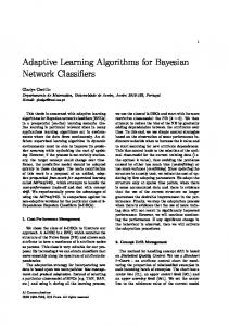
(U) Supervised learning infers a functional relation y = f (x) from a set of training examples D = {(x1 , y1 ), . . . , (xi , yi ), . . . , (xn , yn )}. In what follows the inputs are vectors, e.g. xi = [xi,1 , . . . , xi,j , . . . , xi,d ]T in 0 and yi = −1 if zi ≤ 0. It is straightforward to show that the yi are then independent Bernoulli variables with p(yi = 1) = Φ(β T xi ), i = 1, . . . , n, and we recover the standard probit model. Figure 1 shows the corresponding graphical Markov model using the BUGS plate notation (Spiegelhalter et al., 1999). Specifically, circular vertices in the graph represent random variables whereas sqaure vertices represent constants. The upper rectangle is shorthand for d pairs τj → βj , j = 1, . . . , d with d incoming arrows one into each τj from γ. Similarly in the lower rectangle zi → yi , i = 1, . . . , n is replicated n times. There are arrows from every βj , j = 1, . . . , d to every zi , i = 1, . . . , n. The graph renders the model’s conditional independence assumptions explicitly; each random variable is conditionally independent of its non-descendents given its parents. For example, each yi is conditionally independent of each βj and τj , as well as γ given the corresponding zi . (U) Observe that if z = [z1 , . . . , zi , . . . , zn ] was known, we would have a normal (Gaussian) linear regression, rather than probit regression, problem. Also, if the τ = [τ1 , . . . , τj , . . . , τd ] were known (for any of the hierarchical priors we discuss), we would have a known multivariate Gaussian prior for β, i.e. the same situation as with the nonhierarchical Gaussian prior. Linear regression with a multivariate Gaussian prior on β leads to a closed form (in fact multivariate Gaussian) posterior distribution for β (Gelman et al., 1995). Finding the MAP estimate for β would be easy in this case. (U) The difficulty is that z and τ are latent rather than known. However, given the data yi ˆ for β, the zi have a truncated normal distribution. Similarly, for and a particular choice β all the hierarchical models discussed, the distributions for the τj are known. This situation, where parameters of interest have a tractable distribution when latent variables are known, and latent variables have a tractable distribution when the parameter is known, enables

UNCLASSIFIED

9

Figure 1: (U)Probit Model with Hierarchical Prior and Latent Variables. the use of the Expectation Maximization (EM) algorithm to find the MAP estimate of the parameters. We now describe how the EM algorithm is applied to our models of interest.

3.1

(U) EM for Laplace (Normal-Exponential Hierarchial) Prior

(U) For the latent variable representation for probit under the Laplace prior, both z and τ are latent. The complete data log-posterior is: log p(β|y, τ , z) ∝ log p(z|β) + log p(β|τ ) T

T

(11) T

∝ −β X (Xβ − 2z) − β Γβ,

(12)

where Γ = diag(τ1−1 , . . . , τj−1 , . . . , τd−1 ) is the covariance matrix for the Gaussian prior on β, and X is the design matrix whose rows are x1 T , . . . , xi T , . . . , xn T . Note the complete data log-likelihood is linear in z. (U) The EM algorithm cycles through two steps. The first, or E-step, computes the new expected values for the latent variables given the current estimates of the model parameters. ˆ(t) , y, γ] for each τj , j = On iteration t + 1 of the algorithm, the E-step computes E[τj−1 |β

UNCLASSIFIED

10

ˆ(t) , y, γ] for each zi , i = 1, . . . , n. Here β ˆ(t) is the estimate of β 1, . . . , d, and computes E[zi |β produced at step t of the computation. (U) The distribution of τj is: ˆ(t) , y, γ) = p(τj |βˆj (t) , γ) ∝ p(βˆj (t) |τj )p(τj |γ). p(τj |β

(13)

(U) Defining ωjt+1 to be our desired expected value we then have: ωjt+1

≡

ˆ(t) , y, γ] E[τj−1 |β

= =

R∞

(t) 1 p(βˆj |τj )p(τj |γ)dτj τj R∞ ˆ (t) 0 p(βj |τj )p(τj |γ)dτj (t) γ|βˆj |−1 . 0

(U) The zi have a Gaussian distribution with mean β T xi , but left-truncated at zero if yi = 1 and right-truncated at zero of yi = −1. Defining vi to be the expected value of zi we have: vit+1

   

N (β

T

xi ) if yi = 1 T xi ) ˆ , y, γ] = ≡ E[zi |β T  N (β xi )   β T xi + if yi = −1. T Φ(−β xi ) (t)

β T xi +

1−Φ(−β

(14)

(U) Note that the class labels y affect the result through the expected value of z. The E-step of the EM algorithm computes the above conditional expectations, which lead then to these conditional expectations for the covariance matrix Γ and latent variables z: (t)

ˆ , y, γ] = Ωt+1 = diag(ω1t+1 , . . . , ω t+1 ) E[Γ|β d (t) t+1 t+1 t+1 T ˆ = (v1 , . . . , vn ) E[z|β , y, γ] = v

(15) (16)

(U) The M-step plugs the conditional expectations Ωt+1 and v t+1 into the expression for the ˆt+1 that maximizes this posterior probability of β (Equation 8). It then finds the value β posteriori probability. The optimal value can be written in closed form as: ˆ(t+1) = (Ωt+1 + X T X)−1 X T v t+1 . β

(17)

ˆt (U) The E- and M-steps are repeated until convergence, e.g. until successive values of β differ by less than a specified tolerance. The convexity of the posterior distribution ensures that the algorithm converges to the posterior mode (McLachlan and Krishnan, 1996).

UNCLASSIFIED

3.2

11

(U) EM for Jeffreys (Normal-Jeffreys Hierarchical) Prior

(U) The above EM procedure can be used with the Jeffreys prior (Equation 9) as well. The steps are identical to those for the Laplace prior, except that:

ˆ(t) |−2 , . . . , |β ˆ(t) |−2 ). Ω = diag(ω1 , . . . , ωd ) = diag(|β 1 d

(18)

(U) However, because the posterior distribution of β under the Jeffreys prior is not convex, the EM procedure is gauranteed only to converge to a local optimum of the posterior distribution, not necessarily to the mode.

3.3

(U) EM for Nonhierarchical Gaussian Prior

(U) The above EM procedure can also be used with a simple nonhierarchical Gaussian prior on the probit model. In this case τj = σj2 and is known, not estimated. At all steps ωjt+1 is simply set to τj .

4

(U) Methods

(U) We conducted a set of experiments to compare the effectiveness of the Bayesian probit models with a range of standard supervised learning approaches to text classification. In this section we describe the data sets, effectiveness measures, text representations, feature selection, classifiers, and learning algorithms used in our experiments.

4.1

(U) Data Sets

(U) Our experiments used two standard text categorization test collections. One was the ModApte subset of the Reuters−21578 collection of news stories (Lewis, 1997). This data set is available at: http://www.daviddlewis.com/resources/testcollections/reuters21578/

UNCLASSIFIED

12

The ModApte data set contains 7, 769 documents in the training set and 3, 019 in the test set. Documents in the ModApte data set belong to 0 or more of a set of 135 Topic categories. We used only the 10 most frequent categories in our experiments. (U) The second data set is the RCV1-v2 version of Reuters Corpus Version 1, another collection of news stories recently released by Reuters, Inc. The raw Reuters Corpus Version 1 data is available as described at: http://about.reuters.com/researchandstandards/corpus/ The RCV1-v2 version of the data will be made available as an online appendix to a paper (Lewis, et al, 2003) to appear in the Journal of Machine Learning Research (www.jmlr.org). (U) The RCV1-v2 data set contains 804, 414 news stories. We used the LYRL2003 training/test split (Lewis, etal, 2003), which gives 23,149 training documents and 781,265 test documents. (U) There are 103 Topic categories assigned to RCV1-v2 documents. Our experiments used the 101 Topic categories with one or more positive training examples on our training set. Each RCV1-v2 document belongs to one or more of these categories.

4.2

(U) Effectiveness Measure

(U) We measured effectiveness of our classifier using the so-called “F1-measure,” the harmonic mean of precision and recall (Lewis, 1995). Precision and recall are standard measures used in the text categorization literature:

precision =

recall =

true positive × 100, true positive + false positive

true positive × 100. true positive + false negative

(19)

(20)

UNCLASSIFIED

4.3

13

(U) Text Representation

(U) Text representation refers to the process of converting the raw document text to feature vectors appropriate for a supervised learning algorithm.

4.3.1

(U) ModApte

(U) For the ModApte data set we discarded punctuation marks from the text, then broke the text into indexing terms at whitespace boundaries. After discarding stop words (low content words) from a standard list there were a total of 21,989 unique terms for the ModApte data set. (U) The number of occurrences of each unique term in a document was totaled and became the value of the feature for that document. We refer to feature values computed in this fashion as TF (term frequency) values. A document was therefore represented as a vector of 21,989 integer feature values. Of course, most of the values were 0 for any given document, since any given document contains only a small fraction of the total number of terms. We therefore used sparse storage methods to avoid explicitly representing these 0 values. (U) We also experimented with an alternate method of computing feature values, Log TF weighting. The log TF weights of a term is 0 when the TF is 0, and is equal to 1 + loge (T F ) when TF is greater than 0. Log TF weights take into account the informal notion that the second and subsequent appearances of a word in a document are less informative than the first appearance. Log TF weights tend to improve effectiveness whenever documents are more than a paragraph or two in length. (U) In the next section we compare our results in some places with published results for other learning algorithms on the ModApte data set. The published results have been produced using different text representations than ours, and thus the comparisons are not purely of the learning algorithms.

UNCLASSIFIED 4.3.2

14

(U) RCV1-v2

(U) Text representation for RCV1-v2 used the stemmed token files distributed with the online version of the RCV1-v2 paper (Lewis, et al., 2003). Term weighting was as with the ModApte data set.

4.4

(U) Feature Selection

(U) While our goal in developing the Bayesian algorithms is to eventually eliminate the need for ad hoc feature selection methods, our current implementations of those algorithms are not efficient enough to apply to the full feature sets of the ModApte and RCV1-v2 collections. We there chose for each category a smaller set of features. The features with the largest magnitudes (i.e. highest absolute values) of r, the Pearson product-moment correlation (Diekhoff, 1992) were selected and the others discarded. For feature j this value is: rj = qP

Pn

i=1 (xij

n i=1 (xij

− x(j) )(yi − y)

− x(j) )2

qP n

,

(21)

2 i=1 (yi − y)

where x(j) = [x1,j , . . . , xi,j , . . . , xn,j ]T is the vector of TF or log TF values (see below) for the j-th term. The value x(j) is the mean of xij across the training documents. The yi ’s are the +1/ − 1 class labels for the category being studied, while y is their mean across the training documents. (U) For the experiments reported here, we chose between 300 and 3,000 features for each category depending on the algorithm studied and the data set used. We should note that the Pearson statistic is not widely used for feature selection in text categorization, but our preliminary experiments found it to be more effective than more usual statistics such as chi-square.

4.5

(U) Classifiers and Learning Algorithms

(U) Our main classifiers of interest were probit models with parameters fit under either a Laplace or Jeffreys prior. We also looked at the probit model with a nonhierarchical Gaussian prior. We found the MAP estimate for β for all these models using the EM algorithm described earlier.

UNCLASSIFIED

15

(U) Recall that probit models output not a class label, but an estimate of p(y = 1|β, xi ), the probability that vector xi belongs to the category of interest. To convert the probit model to a classifier, we chose a threshold for each probit model. If p(y = 1|β, xi ) for a test document exceeds the threshold, then a prediction of y = 1 (assign the category) is made. Otherwise a prediction of y = −1 (do not assign the category) is made. (U) We computed a threshold for each category by sorting the training documents on the probit model scores, and finding where this ranking should be separated into two sections to give the smallest number of errors (misclassified training documents). The threshold was set to halfway between the scores of the lowest scoring document in the section assigned to the category and the highest scoring document in the section not assigned to the category. If the smallest number of errors was obtained by putting no documents in the category, then 1.0 plus the score of the highest scoring document was chosen as the threshold. It should be noted that choosing a threshold in this manner is not optimal for the F1 measure, and indeed exactly optimizing F1 requires an approach more complex than thresholding (Lewis, 1995). (U) The other approach we implemented was a logistic regression model with either a (nonhierarchical) Gaussian prior or the (hierarchical) Laplace prior. The MAP estimate of β for the logistic regression model with Gaussian prior was found using our implementation of a published column-relaxation algorithm (Zhang & Oles, 2001). We also modified the Zhang & Oles algorithm to handle the Laplace prior as well. Thresholds for the logistic regression models were chosen in the same fashion as for probit models. (U) We also compare our learning algorithms with published ones on the same data sets, as discussed in the next section.

5

(U) Results

(U) Table 1 and Figure 2 show the performance of the probit model with Laplace prior on the ModApte subset of Reuters-21578. We compare with published results (Zhang & Oles, 2001) for Naive Bayes, logistic regression (with nonhierarchical Gaussian prior), and support vector machines (SVM) on the same data set. (U) Since the algorithms Zhang & Oles tested were particularly efficient, they were able

UNCLASSIFIED

16 Topic

Naive Bayes

SVM

96.6 91.7 70.0 76.7 84.1 52.3 68.2 58.1 76.4 52.4

Logistic (Gaussian) 98.4 95.2 75.2 88.4 85.9 72.9 78.2 88.2 81.9 88.7

98.1 95.3 74.4 89.6 84.8 73.4 75.9 88.9 82.4 86.2

Probit (Laplace) 96.9 90.3 65.9 91.7 81.3 76.7 51.8 89.6 78.8 90.9

earn acq money-fx grain crude trade interest wheat ship corn macro-average micro-average

72.6 85.2

85.3 91.4

84.9 91.1

81.4 88.6

Table 1: (U)F1 Performance results for the ModApte version of Reuters-21578. The Naive Bayes, logistic regression, and SVM results are Zhang & Oles’ published results, using 10,000 features and their text processing. The Probit results use our text processing, log TF weighting, and 300 features selected by Pearson’s correlation. Bold-face indicates the top performer for each category. to do minimal feature selection, keeping 10,000 features. We were able to use only 1,000 features per category for our results, potentially placing the probit model at a disadvantage. Nonetheless, the probit model is competitive for all categories except the interest catgeory. This may be related to the large number of low frequency digit strings (e.g. 3.37 in the context 3.37 pct) that are useful predictors for this category. (U) We conducted a variety of experiments to explore different tunable aspects of the sparse Bayesian algorithm. (U) Table 2 compares raw TF and log TF text representations for probit models with Jeffreys and Laplace (with γ = 10) priors. The log TF is preferable in almost all cases. (U) Table 3 compares Laplace and Jeffreys priors for the probit model. While the Laplace prior requires choosing a hyperparameter (γ) not needed with the Jeffreys prior, the ef-

17

80 70 50

60

F1 Measure

90

100

UNCLASSIFIED

Log.Reg.

NB

Sparse Bayes

SVM

Classifier

Figure 2: (U)Boxplots of Table 1’s results. Each boxplot shows, from top to bottom, the maximum, 75th percentile, median, 25th percentile, and minumum F1 measure across the 10 categories.

UNCLASSIFIED

18

Topic

Jeffreys raw TF

Jeffreys log TF

Laplace γ = 10 Laplace γ = 10 raw TF log TF

earn acq money-fx grain crude trade interest wheat ship corn

96.6 87.7 55.0 89.9 77.7 67.5 49.0 89.7 68.9 88.2

97.1 89.1 59.7 92.3 81.1 71.6 43.9 89.7 67.1 90.3

96.9 89.3 59.3 88.4 82.4 65.4 49.5 87.9 73.0 83.6

96.9 90.3 65.9 91.7 81.3 76.7 51.8 89.6 78.8 90.9

macro-average micro-average

77.0 86.0

78.2 87.4

77.6 87.1

81.4 88.6

Table 2: (U)Comparison of TF and log TF text representations for the probit model with Jeffreys prior and with Laplace prior (γ = 10). Results are shown (and averaged) for the 10 most frequent categories on the ModApte version of Reuters-21578.

UNCLASSIFIED

19

Topic

Jeffreys

Laplace γ = 0.1

Laplace γ = 0.3

Laplace γ=1

Laplace γ=3

Laplace γ = 10

Laplace γ = 30

earn acq money-fx grain crude trade interest wheat ship corn

97.1 89.1 59.7 92.3 81.1 71.6 43.9 89.7 67.1 90.3

97.4 90.5 59.3 88.9 78.9 66.1 56.7 84.0 59.7 83.9

97.5 90.0 60.4 88.1 82.3 67.2 53.1 83.8 65.3 84.9

97.5 90.4 64.3 90.6 80.1 70.5 62.7 86.3 71.9 87.3

97.4 91.7 61.8 90.7 82.2 73.8 50.3 87.2 75.8 91.4

96.9 90.3 65.9 91.7 81.3 76.7 51.8 89.6 78.8 90.9

96.6 89.0 56.8 90.0 76.0 69.5 54.2 89.6 76.3 90.2

macro-average micro-average

78.2 87.4

76.5 87.0

77.3 87.2

80.2 88.2

80.2 88.7

81.4 88.6

78.8 87.0

Table 3: (U)Role of priors. Jeffreys prior compared with Laplace priors with different values of γ. Results for the ModApte version of Reuters-21578. Bold-face indicates the top performer(s) in each row. fectiveness of the resulting classifier is not terribly sensitive to the exact value chosen. In particular, values of γ in the range from 1 to 10 produce competitive results for all categories. (U) Table 4 shows the sparsity achieved with different priors. Choosing, for example, γ = 10 results in substantial sparsity; anywhere from 27% (earn) to 86% (wheat) of the estimated regression co-efficients are zero. Nonetheless, the predictive effectiveness remains competitive. Given the nature of sparsifying priors, it is likely that very similar numbers of features would have been retained even if all 21,989 features had been used as inputs. (U) The data in Table 5 is relevant to two questions. First, is the ad hoc feature selection we did for efficiency in these experiments causing us to substantially underestimate the effectiveness of the probit model? With the Jeffreys prior, this is clearly not the case, since making more features decreases effectiveness more often than it increases it. For the Laplace prior going to 1,000 features increases effectiveness for 8 of 10 categories, and increases average effectiveness by a small amount. Here it appears that the use of 300 features may be limiting effectiveness by a small amount, though a few categories are seriously affected.

UNCLASSIFIED

20

Topic

Jeffreys

Laplace γ = 0.1

Laplace γ = 0.3

Laplace γ=1

Laplace γ=3

Laplace γ = 10

Laplace γ = 30

earn acq money-fx grain crude trade interest wheat ship corn

55 67 32 15 25 20 22 3 19 6

301 301 200 280 282 291 294 275 275 259

300 299 291 251 266 282 270 203 240 232

288 284 276 192 205 261 249 127 176 170

256 257 235 142 174 214 205 90 134 110

220 226 177 92 90 147 136 41 96 47

186 195 111 46 62 80 85 14 55 17

Table 4: (U)Sparsity achieved depending on type and parameter of prior. With 301 input parameters (300 selected features plus intercept), the table shows the number of parameters remaining (i.e., the number of parameters with non-zero posterior modes). Note that sparsity increases with γ, as expected. Results are for the ModApte version of Reuters-21578. (U) The second, and more fundamental, question is whether the sparsifying priors eliminate the need for feature selection from an effectiveness standpoint. That is, can we achieve the desirable properties that feature selection normally provides solely with the Bayesian approach. Again the data is mixed, with it appearing the Jeffreys prior is benefiting slightly from reducing features from 1,000 to 300, while the Laplace prior does not need, and in fact is hurt by feature selection. The real test would be to fit models using the entire feature set, but this is beyond the capability of our current implementation. (U) Another question is whether by requiring a model to be sparse, for efficiency, we give up effectiveness that would be available with a dense model. Table 6 compares densifying (nonhierarchical Gaussian) and sparsifying (Laplace) priors used with the probit and logistic models. Results are mixed, but certainly do not show a clear penalty from sparse models. (U) Tables 7 and 8 revisit some of the same issues using the larger RCV1-v2 collection. Most observations made on the previous collection still hold here. The Laplace prior outperforms the Jeffreys prior. Effectiveness measures show little decline when moving from non-sparse to sparse models. Logistic regression has an advantage over the probit even when the same

UNCLASSIFIED

21

Topic

Jeffreys 300 features

Jeffreys 1000 features

Laplace γ = 10 Laplace γ = 10 300 features 1000 features

earn acq money-fx grain crude trade interest wheat ship corn

97.1 89.1 59.7 92.3 81.1 71.6 43.9 89.7 67.1 90.3

96.8 90.0 63.7 90.8 76.6 62.9 56.0 89.7 66.7 90.3

96.9 90.3 65.9 91.7 81.3 76.7 51.8 89.6 78.8 90.9

97.2 92.2 70.2 91.7 82.5 72.8 63.6 88.9 79.7 90.0

macro-average micro-average

78.2 87.4

78.4 87.3

81.4 88.6

82.9 89.6

Table 5: (U)Role of the number of features. For each of Jeffreys prior and Laplace prior with γ = 10, two runs are compared: with 300 and 1,000 features selected by Pearson’s correlation coefficient. Results for the ModApte version of Reuters-21578.

UNCLASSIFIED

22

Topic

Probit Gaussian

Probit Laplace

Logistic Gaussian

Logistic Laplace

earn acq money-fx grain crude trade interest wheat ship corn

96.8 89.2 65.1 85.1 82.9 71.1 58.1 89.0 83.3 86.7

96.9 90.3 65.9 91.7 81.3 76.7 51.8 89.6 78.8 90.9

97.6 94.0 74.9 91.8 85.7 67.6 67.9 87.7 79.2 90.4

97.8 92.7 64.2 90.7 85.9 70.5 67.3 85.7 78.0 90.4

macro-average micro-average

80.7 87.9

81.4 88.6

83.7 90.7

82.3 89.8

Table 6: (U)Comparing sparse and non-sparse binary regression with F1 measure. Gaussian priors used variance σ 2 = 0.01; Laplace priors used γ = 10 for probit, γ = 100 for logistic. The text representation used for logistic regression incorporated inverse document frequency weights, so the difference in results is not solely due to choice of model. All runs used 300 features selected by the Pearson correlation. Results for the ModApte version of Reuters21578.

UNCLASSIFIED

23 SVM kNN Rocchio

Macro-average Micro-average

61.9 81.6

56.0 76.5

Probit Jeffreys

Probit Logistic Laplace Laplace γ = 25 γ = 625 300 features 300 features 3,000 features

50.4 69.3

39.4 72.5

47.7 74.4

53.0 78.9

Table 7: (U)Effectiveness of sparse Bayesian models compared with that of standard text categorization approaches. The results for SVM (support vector machine), kNN (k-nearest neighbor), and Rocchio classifiers are as reported by Lewis, et al (2003). They use a different text representation than our experiments and so the comparison is not purely of learning algorithms. F1 values are averages over 101 “Topics” categories on the RCV1-v2 collection.

Method Priors

Probit Jeffreys

Features

300

Probit Laplace γ = 25 300

Macro-average Micro-average

39.4 72.5

47.7 74.4

Probit Logistic Logistic Gaussian Laplace Laplace σ 2 = 0.001 γ = 625 γ = 625 300 300 3,000 45.3 74.9

48.0 75.5

53.0 78.9

Logistic Gaussian σ 2 = 0.01 3,000 51.8 79.7

Table 8: (U)Effectiveness of sparse and non-sparse binary regression methods. F1 values are averages over 101 “Topics” categories on the RCV1-v2 collection. number of features is used by both methods. Notice that in contrast with the sparse probit model, logistic regression performance improves significantly as the number of features increases. (U) One substantial difference between the RCV1-v2 and ModApte results is that macroaveraged effectiveness for the sparse models lags that of SVMs by a larger margin on RCV1-v2. The many differences (text representation, feature selection, thresholding) between the published RCV1-v2 experiments and ours mean, however, that no definitive conclusion can be drawn without further experimentation.

UNCLASSIFIED

6

24

(U) Discussion and Future Work

(U) Our experiments indicate that the sparse Bayesian approach is competitive with stateof-the-art techniques for text categorization. The logistic version of the model seems to outperform the probit version. Further, there is some evidence that using a Laplace prior may eliminate the need for ad hoc feature selection. More experimentation is necessary, but initial results are promising. (U) We are currently investigating several topics related to this work. We are developing a block-EM algorithm (Meng and Rubin, 1993) that sequentially updates sub-vectors of β. Note that Equation 17 requires inversion of a d × d matrix, a prohibitively expensive operation for large d. The block-EM algorithm instead requires inversion of several smaller matrices and can provide significant computational savings. Eventually we hope to be able to use the sparse Bayesian models with no feature selection. (U) In many applications, labeled documents arrive sequentially. This creates a need for algorithms that learn in an online fashion. The goal of online learning in the sparse Bayesian classification context is to sequentially update the posterior distribution of the model parameters as each new labeled example arrives. The Bayesian paradigm supports this operation in a natural fashion; starting from the prior, the first example produces a posterior distribution incorporating the evidence from the first example. This then becomes the prior distribution awaiting the arrival of the second example, and so on. In practice, however, except in those cases where the posterior distribution has the same mathematical form as the prior distribution, some form of approximation is required to carry out the sequential updating. We are currently investigating a number of approaches. Other related research topics include automated hyperparameter selection, embedding the logisitic and probit link functions in a general family, and incorporation of external knowledge via prior distributions.

UNCLASSIFIED

25

Appendix A: Convexity of Posterior Distributions (U) The posterior probability for β and its logarithm are given by

p(y|β)p(β) p(y) log p(β|y) = log p(y|β) + log p(β) − log p(y) p(β|y) =

(U) To investigate convexity, we need to calculate first and second partial derivatives with respect to β. The last term on the right-hand side will have zero derivatives and the second one will vary for different prior settings we are going to consider. We start with the first term. log p(y|β) = log Πni=1 Φ(xTi β)yi Φ(−xTi β)1−yi =

n X

{yi log(Φ(xTi β)) + (1 − yi ) log(Φ(−xTi β))}

i=1

(U) Let wi = xTi β and g(wi ) = log Φ(wi ). Then

n X ∂ log p(y|β) = xij {yi g 0 (wi ) − (1 − yi )g 0 (−wi )} ∂βj i=1 n X ∂ 2 log p(y|β) = xij xik {yi g 00 (wi ) + (1 − yi )g 00 (−wi )} ∂βj ∂βk i=1

or, using matrix notation, ∇2 log p(y|β) = X T GX, where G = Diag(..., yi g 00 (wi ) + (1 − yi )g 00 (−wi ), ...) is a n × n diagonal matrix. Now the concavity of log p(y|β) will follow immediately if we show that diagonal elements of G are all negative, so that ∇2 log p(y|β) is negative-semidefinite. For that purpose we calculate

g 00 (wi ) =

φ0 (wi )Φ(wi ) − φ2 (wi ) . Φ2 (wi )

(22)

UNCLASSIFIED

26

(U) This function is always negative; Figure 1 shows its graph. So obviously all diagonal elements of G are negative as well. (U) Consider now the first setting for the prior: βj ∼ N (0, σ 2 ) j = 1, ..., d (U) The corresponding term in the log posterior and its derivatives take the form −

e log Πdj=1 √

log p(β) =

β2 j 2σ 2

βj2 d =− − log 2πσ 2 2 2 2 2πσ j=1 2σ d X

∂ 2 log p(β) 1 = − 2 2 ∂βj σ 2 ∂ log p(β) = 0, ∂βj ∂βk so that the matrix of second partial derivatives is negative definite, and the log posterior is strictly concave. (U) Next we consider the hierarchical model where βj |τj ∼ N (0, τj ) j = 1, ..., d τj ∼ 1/τj j = 1, ..., d. (U) Then the marginal distribution for β is given by p(β) =

Z

∞

p(β|τ )p(τ )dτ = 0

= Πdj=1

Z

∞ 0

Z

∞ 0

Πdj=1 p(βj |τj )p(τj )dτj

p(βj |τj )p(τj )dτj = Πdj=1

1 |βj |

and its log partial first and second order derivatives are given by log p(β) = −

d X j=1

1 ∂ log p(β) = − ∂βj βj 2 ∂ log p(β) 1 = 2 ∂βj βj2 ∂ 2 log(p(β|y)) = 0. ∂βj ∂βk

log(|βj |)

27

−1.0

−0.8

−0.6

f1(x)

−0.4

−0.2

0.0

UNCLASSIFIED

−10

−5

0

5

10

x

Figure 3: (U)Plot of the f function.

UNCLASSIFIED

28

(U) Note that the partial derivatives can only be evaluated for those β ∈ 0) + γI(βj < 0) ∂βj 2 ∂ log p(β) = 0 ∂βj ∂βk (U) Here again derivatives cannot be evaluated when any of βj equals zero. However concavity is not violated.

Acknowledgements (U) We are grateful to Bill DuMouchel, Colin Mallows, and Ilya Muchnik for helpful discussions. The work of Genkin, Lewis and Madigan was partially supported under funds provided by the KD-D group for a project at DIMACS on Monitoring Message Streams, funded through National Science Foundation grant EIA-0087022 to Rutgers University. The NSF also partially supported Madigan and Lewis’s work through ITR grant DMS-0113236.

UNCLASSIFIED

29

References Albert, J.H. and Chib, S. (1993). Bayesian analysis of binary and polychotomous response data. Journal of the American Statistical Association, 88, 669–679. Chai, K.M.A., Chieu, K.L., and Ng, H.T. (2002). Bayesian online classifiers for text classification and filtering ages. In: Proceedings of the 25th Annual International ACM SIGIR Conference on Research and Development in Information Retrieval, 97 - 104. Chambers, E.A. and Cox, D.R. (1967). Discrimination between alternative binary response models. Biometrika, 54, 573–578. Dempster, A.P., Laird, N.M., and Rubin, D.B. (1977). Maximum lilelihood from incomplete data via the EM algorithm (with discussion). Journal of the Royal Statistical Society (Series B), 39, 1–38. Diekhoff, G. (1992). Statistics for the Social and Behavioral Sciences: Univariate, Bivariate, Multivariate. WCB Publishers, Dubuque. Efron, B., Hastie, T., Johnstone, I. and Tibshirani, R. (2003). Least angle regression. Annals of Statistics, to appear. Figueiredo, M.A.T. (2001). Adaptive sparseness using Jeffreys prior. Neural Information Processing Systems, Vancouver, December 2001. Figueiredo, M.A.T. and Jain, A.K. (2001). Bayesian learning of sparse classifiers. IEEE Computer Society Conference on Computer Vision and Pattern Recognition, Hawaii, December 2001. Fu, W.J. (1988). Penalized Regressions: The Bridge Versus the Lasso. Journal of Computational and Graphical Statistics, 7, 397–418. Gelman, A., Carlin, J.B., Stern, H.S., and Rubin, D.B. (1995). Bayesian Data Analysis. Chapman and Hall, London. Girosi, F. (1998). An equivlance between sparse approximation and support vector machines. Neural Computation, 10, 1445–1480.

UNCLASSIFIED

30

Hoerl, A.E. and Kennard, R.W. (1970). Ridge regression: Biased estimation for nonorthogonal problems. Technometrics, 12, 55–67. Joachims, T. (1998). Text Categorization with Support Vector Machines: Learning with Many Relevant Features Proceedings of ECML-98, 10th European Conference on Machine Learning, 137–142. Ju, W., Madigan, D., and Scott, S. (2002). On sparse Bayesian classifiers. DIMACS Technical Report xxx, http://www.stat.rutgers.edu/ madigan/PAPERS/sparse3.pdf Lewis, D.D. (1997). Reuters-21578 text Categorization test collection. Distribution 1.0. README file (v 1.2). Manuscript, 26 September 1997. URL: http://www.daviddlewis.com/resources/testcollections/reuters21578/readme.txt Lewis, D.D. (1998). Naive (Bayes) at forty: The independence assumption in information retrieval. In: ECML’98, The Tenth European Conference on Machine Learning, 4–15. Lewis, D.D. (2002). Applying support vector machines to the TREC-2001 batch filtering and routing tasks. In The Tenth Text REtrieval Conference (TREC 2001), 286–292. Lewis, D. D., Yang, Y., Rose, T., Li, F. (2003). RCV1: A new benchmark collection for text categorization research. Journal of Machine Learning Research, to appear. McLachlan, G.J. and Krishnan, T. (1996). The EM algorithm and extensions, Wiley. Neal, R.M. and Hinton, G.E. (1998). A new view of the EM algorithm that justifies incremental, sparse and other variants. In: Learning in Graphical Models, M.I. Jordan (Editor). Kluwer Academic Publishers, 355–368. Opper, M. (1998). A Bayesian approach to online learning. In: On-Line Learning in Neural Networks, D. Saad (Editor, Cambridge University Press. Osborne, M.R., Presnell, B., and Turlach, B.A. (2000). On the LASSO and its Dual. Journal of Computational and Graphical Statistics, 9,319–338. Ridgeway, G. and Madigan, D. (2003). A sequential Monte Carlo Method for Bayesian analysis of massive datasets. In Journal of Data Mining and Knowledge Discovery, to appear.

UNCLASSIFIED

31

Rocchio, J. (1971). Relevance feedback information retrieval. In: Gerard Salton, editor, The Smart Retrieval System-Experiments in Automatic Document Processing. PrenticeHall, 313–323. Sato, M. and Ishii, S. (2000). On-line EM algorithm for the normalized gaussian network. Neural Computation, 12, 407–432. Sebastiani, F. (2002). Machine learning in automated text categorization. ACM Computing Surveys, 34, 1–47. Smith, A.F.M. and Makov, U. (1978). A quasi-Bayes sequential procedure for mixtures. Journal of the Royal Statistical Society (Series B), 40, 106–112. Smith, R.L. (1999). Bayesian and frequentist approaches to parametric predictive inference (with discussion). In: Bayesian Statistics 6, edited by J.M. Bernardo, J.O. Berger, A.P. Dawid and A.F.M. Smith. Oxford University Press, pp. 589-612. Spiegelhalter, D.J., Thomas, A., and Best, N.G. (1999). WinBUGS Version 1.2 User Manual. MRC Biostatistics Unit. Tibshirani, R. (1995). Regression shrinkage and selection via the lasso. Journal of the Royal Statistical Society (Series B), 58, 267-288. Tipping, M.E. (2001). Sparse Bayesian learning and the relevance vector machine. Journal of Machine Learning Research, 1, 211-244. Titterington, D.M. (1984). Recursive parameter estimation using incomplete data, Journal of the Royal Statistical Society (Series B), 46, 257–267. Yang, Y. (1999). An evaluation of statistical approaches to text categorization and retrieval. Information Retrieval Journal, 1, 69–90. Zhang, T. and Oles, F. (2001). Text categorization based on regularized linear classifiers. Information Retrieval, 4, 5–31.