Sparse Directional Image Representations using the Discrete Shearlet Transform
Glenn Easley System Planning Corporation, Arlington, VA 22209, USA
Demetrio Labate ∗,1 Department of Mathematics, North Carolina State University, Campus Box 8205, Raleigh, NC 27695, USA
Wang–Q Lim Department of Mathematics, Washington University, St. Louis, Missouri 63130, USA
Abstract In spite of their remarkable success in signal processing applications, it is now widely acknowledged that traditional wavelets are not very effective in dealing multidimensional signals containing distributed discontinuities such as edges. To overcome this limitation, one has to use basis elements with much higher directional sensitivity and of various shapes, to be able to capture the intrinsic geometrical features of multidimensional phenomena. This paper introduces a new discrete multiscale directional representation called the Discrete Shearlet Transform. This approach, which is based on the shearlet transform, combines the power of multiscale methods with a unique ability to capture the geometry of multidimensional data and is optimally efficient in representing images containing edges. We describe two different methods of implementing the shearlet transform. The numerical experiments presented in this paper demonstrate that the Discrete Shearlet Transform is very competitive in denoising applications both in terms of performance and computational efficiency. Key words: Curvelets, denoising, image processing, shearlets, sparse representation, wavelets 1991 MSC: 42C15, 42C40
Preprint submitted to Elsevier
on June 12, 2006; revised on August 4, 2007
1
Introduction
One of the most useful features of wavelets is their ability to efficiently approximate signals containing pointwise singularities. Consider a one-dimensional signal s(t) which is smooth away from point discontinuities. If s(t) is approximated using the best M -term wavelet expansion, then the rate of decay of the approximation error, as a function of M , is optimal. In particular, it is significantly better than the corresponding Fourier approximation error [14,32]. However, it is now widely acknowledged that traditional wavelet methods do not perform as well with multidimensional data. Indeed wavelets are very efficient in dealing with pointwise singularities only. In higher dimensions, other types of singularities are usually present or even dominant, and wavelets are unable to handle them very efficiently. Images, for example, typically contain sharp transitions such as edges, and these interact extensively with the elements of the wavelet basis. As a result, “many” terms in the wavelet representation are needed to accurately represent these objects. In order to overcome this limitation of traditional wavelets, one has to increase their directional sensitivity and a variety of methods for addressing this task have been proposed in recent years. They include several schemes of “directional wavelets” (such as [1,3]), contourlets [12,31], complex wavelets [25,34] brushlets [9], ridgelets [6], curvelets [7], bandelets [29] and shearlets [20,18], introduced by the authors and their collaborators. To make this discussion more rigorous, it will be useful to examine this problem from the point of view of approximation theory. If F = {ψµ : µ ∈ I} is a basis or, more generally, a tight frame for L2 (R2 ), then an image f can be (nonlinearly) approximated by the partial sums fM =
X
hf, ψµ i ψµ ,
µ∈IM
where IM is the index set of the M largest inner products |hf, ψµ i|. The resulting approximation error is εM = kf − fM k2 =
X
|hf, ψµ i|2 ,
µ∈I / M
and this quantity approaches asymptotically zero as M increases. For many signal processing applications, the goal is to design the representation system ∗ Corresponding author Email addresses:
[email protected] (Glenn Easley),
[email protected] (Demetrio Labate),
[email protected] (Wang–Q Lim). 1 Partially supported by National Science Foundation grant DMS 0604561.
2
F that achieves the best asymptotic decay rate for this error. For example, for compression applications it has been shown that the distortion rate is proportional εM [17]. Similarly, the efficiency of noise removal algorithms that use thresholding estimators have been shown to depend upon εM [15]. Let C 2 be the space of functions that are twice continuously differentiable. If the image f is C 2 , then the approximation fM obtained from the M largest wavelet coefficients satisfies εM ≤ C M −2 . However, images typically contain edges. If f is C 2 everywhere away from edge curves that are piecewise C 2 , then the discontinuity creates many wavelet coefficients of large amplitude. As a result (see [32]), the asymptotic approximation error obtained using wavelets only decays as: εM ≤ C M −1 . This is better than Fourier approximations (in which case the error decays as M −1/2 ), but far from the theoretical optimal approximation, where εM decays as M −2 [13]. This shows that one can improve upon the wavelet representation by appropriately exploiting the geometric regularity of the edges. Indeed, Cand`es and Donoho have recently introduced the curvelet representation, a tight frame of elongated oscillatory functions at various scales, that produce an essentially optimal approximation rate [7]. Namely, it satisfies εM ≤ C (log M )3 M −2 .
(1.1)
However, curvelets are not generated from the action of a finite family of operators on a single function, as is the case with wavelets. This means their construction is not associated with a multiresolution analysis. This and other issues make the discrete implementation of curvelets very challenging as is evident by the fact that two different implementations of it have been suggested by the originators (see [35] and [5]). In an attempt to provide a better discrete implementation of the curvelets, the contourlet representation has been recently introduced [11,31,33]. This is a discrete time-domain construction, which is designed to achieve essentially the same frequency tiling as the curvelet representation (observe however that the contourlets are not a ‘discretization’ of curvelets). The authors of this paper and their collaborators have recently introduced the shearlet representation [18–22], which yields the same optimal approximation properties (1.1). This new representation is based on a simple and rigorous mathematical framework which not only provides a more flexible theoretical 3
tool for the geometric representation of multidimensional data, but is also more natural for implementation. In addition, the shearlet approach can be associated to a multiresolution analysis [22,27]. In this paper, we will develop discrete implementations of the shearlet transform to obtain the Discrete Shearlet Transform. We will show that the mathematical framework of the shearlet transform allows us to develop a simple and faithful transition from the continuous to the discrete representation. It will become clear from our constructions that the shearlet approach can be viewed as a simplifying theoretical justification for the contourlet transform. The shearlet transform, however, offers a much more flexible approach, and allows one to develop a variety of alternative implementations, with complete control over the mathematical properties of the transform, and features that can be adapted to specific applications. The paper is organized as follows. In Section 2 we describe the mathematical theory of shearlets and its connection with the theory of affine systems with composite dilations. In Section 3 we introduce the Discrete Shearlet Transform. Finally, in Section 4, we present several demonstrations of the Discrete Shearlet Transform for noise removal applications. Concluding remarks are made in Section 5.
2
Shearlets
The theory of composite wavelets, recently introduced by the authors and their collaborators [20–22], provides an especially effective approach for combining geometry and multiscale analysis by taking advantage of the classical theory of affine systems. In dimension n = 2, the affine systems with composite dilations are the collections of the form: AAB (ψ) = {ψj,`,k (x) = | det A|j/2 ψ(B ` Aj x − k) : j, ` ∈ Z, k ∈ Z2 },
(2.2)
where ψ ∈ L2 (R2 ), A, B are 2 × 2 invertible matrices and | det B| = 1. The elements of this system are called composite wavelets if AAB (ψ) forms a Parseval frame (also called tight frame) for L2 (R2 ); that is, X
|hf, ψj,`,k i|2 = kf k2 ,
j,`,k
for all f ∈ L2 (R2 ). In this approach, the dilations matrices Aj are associated with scale transformations, while the matrices B ` are associated to area-preserving geometrical transformations, such as rotations and shear. This framework allows one to construct Parseval frames whose elements range not only at various scales and locations, like wavelets, but also at various orientations. 4
In this paper, we will consider a special example of composite wavelets in L2 (R2 ), called shearlets. These are collections of the form (2.2) where A = A0 is the anisotropic dilation matrix and B = B0 is the shear matrix, which are given by 4 0 A0 = , 02
1 1 B0 = . 01
b 2 , ξ 6= 0, let ψ (0) be given by For any ξ = (ξ1 , ξ2 ) ∈ R 1 Ã
ˆ(0)
ˆ(0)
ψ (ξ) = ψ (ξ1 , ξ2 ) = ψˆ1 (ξ1 ) ψˆ2
!
ξ2 , ξ1
(2.3)
b supp ψ ˆ1 ⊂ [− 1 , − 1 ] ∪ [ 1 , 1 ] and supp ψˆ2 ⊂ [−1, 1]. where ψˆ1 , ψˆ2 ∈ C ∞ (R), 2 16 16 2 This implies that ψˆ(0) is C ∞ and compactly supported with supp ψˆ(0) ⊂ [− 21 , 12 ]2 . In addition, we assume that X
|ψˆ1 (2−2j ω)|2 = 1
j≥0
1 for |ω| ≥ , 8
(2.4)
and, for each j ≥ 0, j −1 2X
|ψˆ2 (2j ω − `)|2 = 1
for |ω| ≤ 1.
(2.5)
`=−2j
From the conditions on the support of ψˆ1 and ψˆ2 one can easily observe that the functions ψj,`,k have frequency support: (0) supp ψˆj,`,k ⊂ {(ξ1 , ξ2 ) : ξ1 ∈ [−22j−1 , −22j−4 ]∪[22j−4 , 22j−1 ], | ξξ12 +` 2−j | ≤ 2−j }.
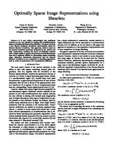
That is, each element ψˆj,`,k is supported on a pair of trapezoids, of approximate size 22j × 2j , oriented along lines of slope ` 2−j (see Figure 1(b)). There are several examples of functions ψ1 , ψ2 satisfying the properties described above (see Appendix A.1). The equations (2.4) and (2.5) imply that j −1 X 2X
j≥0 `=−2j
−` 2 |ψˆ(0) (ξ A−j 0 B0 )| =
j −1 X 2X
ξ2 |ψˆ1 (2−2j ξ1 )|2 |ψˆ2 (2j − `)|2 = 1 ξ1 j≥0 `=−2j
b 2 : |ξ | ≥ 1 , | ξ2 | ≤ 1}. That for (ξ1 , ξ2 ) ∈ D0 , where D0 = {(ξ1 , ξ2 ) ∈ R 1 8 ξ1 −j −` (0) ˆ is, the functions {ψ (ξ A0 B0 )} form a tiling of D0 . This is illustrated in Figure 1(a).
This property, together with the fact that ψˆ(0) is supported inside [− 12 , 12 ]2 , 5
ξ2
6
∼ 2j
ξ1
? ¾
2j
∼2
(a)
(b)
b 2 induced by the shearlets. The tiling Fig. 1. (a) The tiling of the frequency plane R of D0 is illustrated in solid line, the tiling of D1 is in dashed line. (b) The frequency support of a shearlet ψj,`,k satisfies parabolic scaling. The figure shows only the support for ξ1 > 0; the other half of the support, for ξ1 < 0, is symmetrical.
implies that the collection: (0)
3j
{ψj,`,k (x) = 2 2 ψ (0) (B0` Aj0 x − k) : j ≥ 0, −2j ≤ ` ≤ 2j − 1, k ∈ Z2 },
(2.6)
is a Parseval frame for L2 (D0 )∨ = {f ∈ L2 (R2 ) : supp fˆ ⊂ D0 }. Details about this can be found in [22]. Similarly we can construct a Parseval frame for L2 (D1 )∨ , where D1 is the b 2 : |ξ | ≥ 1 , | ξ1 | ≤ 1}. Let vertical cone D1 = {(ξ1 , ξ2 ) ∈ R 2 8 ξ2
2 0 A1 = , 04
1 0 B1 = , 11
and ψ (1) be given by Ã
ψˆ(1) (ξ) = ψˆ(1) (ξ1 , ξ2 ) = ψˆ1 (ξ2 ) ψˆ2
!
ξ1 , ξ2
where ψˆ1 , ψˆ2 are defined as above. Then the collection (1)
3j
{ψj,`,k (x) = 2 2 ψ (1) (B1` Aj1 x − k) : j ≥ 0, −2j ≤ ` ≤ 2j − 1, k ∈ Z2 }
(2.7)
is a Parseval frame for L2 (D1 )∨ . Finally, let ϕˆ ∈ C0∞ (R2 ) be chosen to satisfy 6
2
G(ξ) = |ϕ(ξ)| ˆ +
j −1 X 2X
−` 2 |ψˆ(0) (ξA−j 0 B0 )| χD0 (ξ)
j≥0 `=−2j
+
j −1 X 2X
−` 2 |ψˆ(1) (ξA−j 1 B1 )| χD1 (ξ) = 1,
b 2, for ξ ∈ R
j≥0 `=−2j
where χD denotes the indicator function of the set D. This implies that 1 1 2 supp ϕˆ ⊂ [− 81 , 81 ]2 , with |ϕ(ξ)| ˆ = 1 for ξ ∈ [− 16 , 16 ] , and the set {ϕ(x − k) : 1 1 2 ∨ 2 2 k ∈ Z } is a Parseval frame for L ([− 16 , 16 ] ) . Observe that, by the properties of ψ (d) , d = 0, 1, it follows that the function G(ξ) = G(ξ1 , ξ2 ) is continuous b 2 ). and regular along the lines ξ2 /ξ1 = ±1 (as well as for any other ξ ∈ R Thus, we have the following: (d)
3j
Theorem 2.1 Let ϕk (x) = ϕ(x − k) and ψj,`,k (x) = 2 2 ψ (d) (Bd` Ajd x − k), where ϕ, ψ are given as above. Then the collection of shearlets: [
(d)
{ϕk : k ∈ Z2 } {ψj,`,k (x) : j ≥ 0, −2j + 1 ≤ ` ≤ 2j − 2, k ∈ Z2 , d = 0, 1} [ (d) {ψ˜j,`,k (x) : j ≥ 0, ` = −2j , 2j − 1, k ∈ Z2 , d = 0, 1}, (d)
b (d) where ψ˜j,`,k (ξ) = ψbj,`,k (ξ) χDd (ξ), is a Parseval frame for L2 (R2 ). (d) As shown above, the “corner” elements ψ˜j,`,k (x), ` = −2j , 2j − 1, are simply obtained by truncation on the cones χDd in the frequency domain. As mentioned above, the corner elements in the horizontal cone D0 match nicely with those in the vertical cone D1 .
For d = 0, 1, the shearlet transform is mapping f ∈ L2 (R2 ) into the elements (d) hf, ψj,`,k i, where j ≥ 0, −2j ≤ ` ≤ 2j − 1, k ∈ Z2 . Let us summarize the mathematical properties of shearlets: • Shearlets are well localized. In fact, they are compactly supported in the frequency domain and have fast decay in the spatial domain. • Shearlets satisfy parabolic scaling. Each element ψˆj,`,k is supported on a pair of trapezoids, each one contained in a box of size approximately 2j × 22j (see Figure 1(b)). Because the shearlets are well localized, in the spatial domain each ψj,`,k is essentially supported on a box of size 2−j × 2−2j . Their supports become increasingly thin as j → ∞. • Shearlets exhibit highly directional sensitivity. The elements ψˆj,`,k are oriented along lines with slope given by −` 2−j . As a consequence, the corresponding elements ψj,`,k are oriented along lines with slope ` 2−j . The number of orientations doubles at each finer scale. 7
• Shearlets are spatially localized. For any fixed scale and orientation, the shearlets are obtained by translations on the lattice Z2 . • Shearlets are optimally sparse. The following is proved in [19, Thm. 1.1]) : Theorem. Let f be C 2 away from piecewise C 2 curves, and fNS be the approximation to f obtained using the N largest coefficients in the shearlet expansion. Then we have: kf − fNS k22 ≤ C N −2 (log N )3 . Thus the shearlets form a tight frame of well localized waveforms, at various scales and directions, and are optimally sparse in representing images with edges. Only the curvelets of Cand`es and Donoho are known to satisfy similar sparsity properties 2 . With respect to the curvelets, however, our construction has some fundamental differences. Indeed, the shearlets are generated from the action of a family of operators on a single function, while this is not true for the curvelets (they are not of the form (2.2)). In particular, unlike the shearlets, the curvelets are not associated with a fixed translation lattice. Concerning the directional sensitivity, the number of orientations in our construction doubles at each scale, while in the curvelet case it doubles at each other scale. This is consistent with the fact that our √ dilations factors in the dilation matrix A are 4 and 2 rather than 2 and 2, as in the case of curvelets. In addition, the shearlets are defined on the Cartesian domain and the various directions are obtained from the action of shearing transformations. By contrast, the curvelets are constructed in the polar domain and the orientations are obtained by applying rotations. Finally, thanks to their mathematical structure, the shearlets are associated to a multiresolution analysis (see [27,30]). Also the discrete construction of the contourlets introduced by Do and Vetterli [12] has the intent to provide a partition of the frequency plane very similar to the one represented in Figure 1. In this sense, the theory of shearlets can be seen as a theoretical justification for the contourlets. Observe, however, that the shearlets are band-limited functions, while the contourlets are a discretetime construction implemented using filter banks. Indeed, the framework of composite wavelets from which the shearlets are derived allows one to consider directional multiscale representations with compact support [26]. It is an open problem whether one can construct a directional multiscale Parseval frame of functions that are both compactly supported and smooth.
2
Also the contourlets are claimed in [12] to satisfy the same sparsity property. The argument used in [12] assumes that there exist smooth compactly supported functions approximating a frequency partition similar to Figure 1. However, the existence of functions with such properties is an open and nontrivial problem.
8
3
The Discrete Shearlet Transform
It will be convenient to describe the collection of shearlets presented above in a way which is more suitable to derive its numerical implementation. For b 2 , j ≥ 0, and ` = −2j , . . . , 2j − 1, let ξ = (ξ1 , ξ2 ) ∈ R ψˆ (2j ξξ12 − `) χD0 (ξ) + ψˆ2 (2j ξξ21 − ` + 1) χD1 (ξ) 2
Wj,` (ξ) = ψˆ2 (2j ˆ2 (2j ψ (0)
ξ2 ξ1 ξ2 ξ1
− `) χD0 (ξ) + ψˆ2 (2j − `)
ξ1 ξ2
− ` − 1) χD1 (ξ)
if ` = −2j if ` = 2j − 1 otherwise
and
(1) Wj,` (ξ)
=
ψˆ (2j ξξ21 − ` + 1) χD0 (ξ) + ψˆ2 (2j ξξ21 − `) χD1 (ξ) 2
ψˆ2 (2j ξ12 − ` − 1) χD0 (ξ) + ψˆ2 (2j ξ12 − `) χD1 (ξ) ˆ2 (2j ξ1 − `) ψ ξ ξ
ξ
2
if ` = −2j if ` = 2j − 1 otherwise,
where ψ2 , D0 , D1 are defined in Section 2. For 1 − 2j ≤ ` ≤ 2j − 2, each term (d) Wj,` (ξ) is a window function localized on a pair of trapezoids, as illustrated in Figure 1(a). When ` = −2j or ` = 2j − 1, at the junction of the horizontal (d) cone D0 and the vertical cone D1 , Wj,` (ξ) is the superposition of two such functions. Using this notation, for j ≥ 0, −2j ≤ ` ≤ 2j − 1, k ∈ Z2 , d = 0, 1, we can write the Fourier transform of the shearlets in the compact form 3j
−j −` (d) (d) ψˆj,`,k (ξ) = 2 2 V (2−2j ξ) Wj,` (ξ) e−2πiξAd Bd k ,
where V (ξ1 , ξ2 ) = ψˆ1 (ξ1 ) χD0 (ξ1 , ξ2 )+ ψˆ1 (ξ2 ) χD1 (ξ1 , ξ2 ). The shearlet transform of f ∈ L2 (R2 ) can be computed by (d) hf, ψj,`,k i
=
3j 22
Z R2
−j −` (d) fˆ(ξ) V (2−2j ξ) Wj,` (ξ) e2πiξAd Bd k dξ.
(3.8)
Indeed, one can easily verify that j −1 1 2X X
(d)
|Wj,` (ξ1 , ξ2 )|2 = 1,
d=0 `=−2j
and from this it follows that 2
|ϕ(ξ ˆ 1 , ξ2 )| +
j −1 1 X 2X X
(d)
b 2. |V (22j ξ1 , 22j ξ2 )| |Wj,` (ξ1 , ξ2 )|2 = 1 for (ξ1 , ξ2 ) ∈ R
d=0 j≥0 `=−2j
9
3.1 A Frequency-Domain Implementation We will now derive an algorithmic procedure for computing (3.8) in frequency domain which is faithful to the mathematical transformation described above. −1,N −1 An N × N image consists of a finite sequence of values, {x[n1 , n2 ]}N n1 ,n2 =0 where N ∈ N. Identifying the domain with the finite group Z2N , the inner product of images x, y : Z2N → C is defined as
hx, yi =
N −1 N −1 X X
x(u, v)y(u, v).
u=0 v=0
Thus the discrete analog of L2 (R2 ) is `2 (Z2N ). Given an image f ∈ `2 (Z2N ), let fˆ[k1 , k2 ] denote its 2D Discrete Fourier Transform (DFT): 1 fˆ[k1 , k2 ] = N
N −1 X
n1
n1
f [n1 , n2 ] e−2πi( N k1 + N k2 ) ,
n1 ,n2 =0
− N2 ≤ k1 , k2
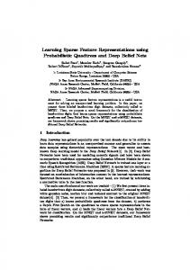
0 so that the decay rate of the nonlinear approximation curve is at least arbitrarily close to 1. Our numerical experiment (see Figure 6(b)) shows that the decay rate of the nonlinear approximation curve for the shearlet transform is close to 1 for our test image shown in Figure 5(a). In this numerical experiment, we compare the non-linear approximation curve for our shearlet 15
0.035
0.03
L2 Error
0.025
Estimated curve: point FST: solid line
0.02
0.015
0.01
0.005
0
(a)
0
0.5
1 1.5 Number of coefficients
2
2.5 6
x 10
(b)
Fig. 6. (a) Original image. (b)Partial reconstruction error kf − fM k/kf k and the numerically estimated curve.
representation and the numerically estimated curve of the form CM −α . For this estimated curve, we obtained α ' 0.9634 which is close to 1. Although there is a redundancy in the number of retained coefficients, the asymptotic decay rate demonstrated above indicates that this discrete implementation should perform well as a denoising routine. An analogous situation occurs for the wavelet transform and its implementation. The success of the wavelet transform for denoising is based on its non-linear approximation error rate and yet their most successful implementations for estimation purposes are typically done by using the highly redundant nonsubsampled version (see, for example, [8,28]).
3.3 A Time-Domain Implementation In order to improve the algorithm performance for applications such as denoising, we need to implement a local variant of the shearlet transform. This will reduce the Gibbs type ringing present when filters of large support sizes are used. Note that the concept of localizing the transform is not new. For example, a localization has been applied to the ridgelet transform in order to implement the discrete curvelet transform [35]. In order to obtain a local variant similar to the one used for ridgelets, we would need to apply the shearlet transforms to small sized image blocks (e.g., blocks of sizes 8 by 8, or 16 by 16). In order to avoid blocking artifacts, we would need to introduce an overcomplete decomposition of the image and then synthesize by a lapped window scheme such as in [35]. Indeed, the added redundancy in the number of shearlet coefficients makes this a cumbersome approach. But a much simpler, faster, and time-domain solution is possible. 16
Recall that in the implementation there is a large flexibility in the choice ˜ of windowing to be applied. Consider a frequency-based window function W P2j −1 ˜ j such that `=−2j W [2 n2 − `] = 1. Denote by ϕP the mapping function from the Cartesian grid to the pseudo-polar grid. The shearlet coefficients in the ˜ j discrete Fourier domain were earlier calculated as ϕ−1 P (gj [n1 , n2 ]W [2 n2 − `]), where gj represents fˆdj in the pseudo-polar domain. We suggest to calculate the shearlet coefficients in the frequency domain as −1 ˆ ˜ j ϕ−1 P (gj [n1 , n2 ])ϕP (δP [n1 , n2 ]W [2 n2 − `]),
where δˆP represents the discrete Fourier transform of the delta function in the pseudo-polar grid. This is possible because the map ϕP can be described as a selection matrix S with the property that its elements si,j satisfy the property s2i,j = si,j (see [10] for more details). In this way, we can calculate the shearlet s coefficients in the discrete Fourier domain as fˆdj [n1 , n2 ]wˆj,` [n1 , n2 ] where s ˆ ˜ j wˆj,` [n1 , n2 ] = ϕ−1 P (δP [n1 , n2 ]W [2 n2 − `]).
The subtle but very important point here is that the new form of the filters are not found by a simple change of variables. They are found by applying the specific discrete re-sampling transformation converting from the pseudopolar to Cartesian coordinate system. This discrete transformation requires a re-sampling, where many points in the pseudo-polar coordinate systems may be mapped into a single point in the Cartesian system. s An illustration of such filters w ˆj,` found by using a Meyer window are shown Figure 7.
1
1
0
0
s constructed using a Meyer wavelet as Fig. 7. Examples of the shearing filters w ˆj,` the window function W . s such that As a result of this conversion we now have filters w ˆj,` j −1 2X
s wˆj,` (ξ1 , ξ2 ) = 1.
`=−2j
17
Because this construction is independent of the image f , we can now construct shearing filters for any size coordinate system. By taking the inverse discrete Fourier transform, we thus have the following theorem: s Theorem 3.1 Let w`s denote the shearing filter w0,` with support size L × L. 2 2 Given any function f ∈ ` (ZN ),
j −1 2X
f ∗ w`s = f.
`=−2j
Although these filters are not compactly supported in the traditional sense, they can be implemented with a matrix representation that is smaller in size than the given image. These observations show that we can perform the shearing filtering “directly” in the time-domain using a convolution. In our implementation, we will restrict the convolution to be of the same size as the given image. In addition, the small support sizes of the filters reduce the Gibbs-type ringing phenomenon and improve the computational efficiency of the algorithm. In fact, the small sized filters allows us to use a fast overlap-add method to compute the convolutions [32]. The gain in speed for the directional filtering combined with the performance of the Laplacian pyramid algorithm used in our routine yields an overall performance of O(N 2 log N ) operations. Another benefit of this implementation is that we can apply a nonsubsampled Laplacian pyramid decomposition which has been shown to be very effective in denoising applications [11]. Although this is a highly redundant decomposition (e.g. the number of retained coefficients for a three-level decomposition would be (2j + 2j−1 + 1)N 2 when 2j directional subbands are chosen at the first decomposition level when applied to an N × N image), this version will be shown to be highly effective for the purpose of denoising. On the other hand, it is useful to observe that the frequency–domain implementation discussed in the previous section allows for a much broader class of wavelet filtering (windowing) to be implemented. This can be useful for other types of applications. Displays of various basis functions for the time-domain implemented shearlet transform are shown in Figure 8. The second level decomposition was divided into 16 directional subbands and the third level decomposition was divided into 8 directional subbands. 18
Fig. 8. Examples of basis functions of the time-domain implemented shearlet transform. The top row corresponds to the basis functions of the second decomposition level. The bottom row corresponds to the basis functions of the third decomposition level.
3.3.1 Comparison with the Contourlets The time-domain shearlet transform that we described above has similarities with the contourlet transform [11,31,33]. Recall that the contourlet transform consists of an application of the Laplacian pyramid followed by directional filtering. However the directional filtering is obtained using a different approach from the shearlets. Indeed, the directional filtering of the contourlet transform is achieved by introducing a directional filter bank that combines critically sampled fan filter banks and pre/post re-sampling operations. An important advantage of the shearlet transform over the contourlet transform is that there are no restrictions on the number of directions for the shearing. That is, we could express the formulation of the windowing W with a non-dyadic spacing as well. This flexibility is not possible using a fan filter implementation. In addition, in the shearlet approach, there are no constraints on the size of the supports for the shearing, unlike the construction of the directional filter banks in [33]. Finally, we wish to point out that the inversion of this discrete shearlet transform only requires a summation of the shearing filters rather than inverting a directional filter bank. This results in an implementation that is most efficient computationally. In addition, this efficient inversion may have advantages for applications such as compression routines where the complexity of the decompression algorithm needs to be minimal.
3.4 Computational Efficiency and Accuracy To give an indication of how computationally efficient the shearlet transform is, we have compared CPU times for computing the shear filtered coefficients 19
(SFC) and its inversion processes (iSFC) to those of the nonsubsampled directional filter bank (DFB) and its inversion process (iDFB) used as part of the nonsubsampled contourlet transform. Our test was based on using a laptop with a 1.73GHz Centrino processor and 1GB of ram. The routines were tested in MATLAB with only one routine of the DFB codes compiled from C. The DFB codes were provided by the authors of the nonsubsampled contourlet transform papers. The sizes of the shearing filters used were 16 × 16. We measured the following CPU times averaged over 10 iterations:
directions
image size
cpu time
SFC
8
512
1.4641 × 100 sec
iSFC
8
512
2.9687 × 10⁻² sec
SFC
16
512
2.9266 × 100 sec
iSFC
16
512
1.0938 × 10⁻¹ sec
DFB
8
512
1.0850 × 10² sec
iDFB
8
512
1.0867 × 10² sec
DFB
16
512
2.7685 × 10² sec
iDFB
16
512
2.7865 × 10² sec
Notice that doubling the number of directions for the shearing processes only marginally increases the computational time, whereas it more than doubles the time for the directional filter bank process. Also, it can be seen that the time to invert the shearing is practically negligible for an image of size 512 × 512. Below are the results for the frequency-domain shearing. directions image size
CPU time
Freq-SFC
8
512
3.8898 × 101 sec
Freq-iSFC
8
512
2.8125 × 10⁻¹ sec
Freq-SFC
16
512
1.2950 × 10² sec
Freq-iSFC
16
512
5.8203 × 10⁻¹ sec
The average CPU time to decompose an image of size 512 via the LP algorithm used in the frequency-domain implementation for the shearlet transform was 3.2656 × 10⁻¹ . The average CPU time to recompose via the LP algorithm was 20
3.2969 × 10⁻¹ . For the nonsubsampled LP algorithm used in the time-domain shearlet transform, the average CPU time was 4.7656 × 10⁻¹ . The average CPU time to recompose was 4.8281 × 10⁻¹ . The relative error in the reconstruction of the frequency-domain implementation for an image of size 512 (Lena) was 3.8842×10⁻¹³ . For the nonsubsampled time-domain shearlet transform, the relative errors were 7.8228×10⁻¹⁶ using a Meyer wavelet-based window and 7.8249×10⁻¹⁶ using a characteristic function based window. These results are acceptable and expected when implemented in a finite precision machine. The frequency-domain implementation only suffers from a slight performance degradation due to the limits on the discretization of the one-dimensional Meyer wavelet being used. The degradation is more visible when used on a signal of length 1024 than for a signal of length 32 or 64. Alternative discretizations of the Meyer wavelet could be used to mitigate this issue.
4
Numerical Experiments
The highly directional sensitivity of the shearlet transform and its optimal approximation properties will lead to improvements in many image processing applications. To illustrate one of its potential uses, we have used the shearlet transform to remove noise from images. Specifically, suppose that for a given image f , we have u=f +² (4.13) where ² is Gaussian white noise with zero mean and standard deviation σ; that is, ² ∈ N (0, σ 2 ). We attempt to recover the image f from the noisy data u by computing an approximation f˜ of f obtained by applying a thresholding scheme in the subbands of the shearlet decomposition. First, we demonstrate the performance in estimation by applying hard thresholding to the subbands of the shearlet decomposition using the frequencybased routine. The decomposition tested is the same as that shown in Figure 3. The result is shown in Figure 9. The performance measure used was the peak signal-to-noise ratio (PSNR) in decibels (dB) defined as P SN R = 20 log10
255N . kf − f˜kF
where k · kF is the Frobenius norm, the given image f is of size N × N , and f˜ denotes the estimated image. Included in this experiment are the estimates found by applying hard thresholding to the discrete wavelet transform defined in terms of the Daubechies-Antonini 7/9 filters and the contourlet transform using a decomposition compatible with the shearlet decomposition. We also 21
(a)
(b)
(c)
(d)
(e)
(f)
Fig. 9. (a) The original cameraman image. (b) The noisy image (PSNR=22.09dB). (c) The result of wavelet denoising using the 7/9 filters (PSNR=26.18dB). (d) The result of contourlet denoising (PSNR=25.82dB). (e) The result of the frequency-based shearlet denoising (PSNR=27.21dB). (f) The result of the time-domain shearlet denoising (PSNR=28.01dB).
22
include the performance when hard thresholding is applied to the time-domain based shearlet transform. The decomposition is the same as for the frequencybased transform but with the shearing filters used to obtain the 8 and 4 directional subbands constructed using filters of size 16 and 32, respectively. This experiment suggests a better performance in using the time-domain shearlet transform for denoising and hence we provide a more complete set of comparisons using this implementation. Taking note of the great performance of the nonsubsampled contourlet transform for image denoising [11], we use a time-domain shearlet transform and choose the threshold parameters 2 τi,j = σ²2i,j /σi,j,n
(4.14)
2 as in [11] where σi,j,n denotes the variance of the n-th coefficient at the ith shearing direction subband in the jth scale, and σ²2i,j is the noise variance at scale j and shearing direction i. Various experiments indicate the shearlet coefficients can be modeled by generalized Gaussian distributions so that these thresholds should yield a risk close to the optimal Bayes risk, specifically within 5 percent of it. To estimate the signal variances in each subband locally, the neighboring coefficients contained in a square window and a maximum likelihood estimator are used. The variances σ²2i,j are estimated by using a Monte-Carlo technique in which the variances are computed for several normalized noise images and then the estimates are averaged.
The particular form of the time-domain based shearlet transform we tested was to use the nonsubsampled Laplacian pyramid transform with several different combinations of the shearing filters. This will be simply referred to as the Nonsubsampled Shearlet Transform (NSST). We use the abbreviation of NSST1 (L1 ,L2 ) and NSST2 (L1 ,L2 ) to indicate the type of windowing used and the support sizes of the shearing filters w`s . In particular, we implemented the shearing on 4 of the 5 scales of the Laplacian pyramid transform decomposition. The shearing filters of sizes L1 × L1 , L1 × L1 , L2 × L2 , and L2 × L2 from finer to coarser were used with the number of shearing directions chosen to be 16, 16, 8, and 8. Note that the only restriction on the construction of the shearing filters is that the maximum number of directional subbands is less than or equal to the size of the filter. NSST1 refers to the case where the shearing was done by using a Meyer wavelet window and NSST2 to the case where the shearing was done with a simple characteristic window function. For example, NSST1 (16,32) indicates that a Meyer-based shearing filter of size 16 with 16 directions was applied to the first and second decomposition level and a Meyer-based shearing filter of size 32 with 8 directions was applied to the third and fourth decomposition level. We tested the denoising schemes using the images shown in Figure 10 for various standard deviation values of the noise. For a baseline comparison, we 23
Fig. 10. Test images. From top left, clockwise: Lena, Peppers, Elaine, and Goldhill.
tested the performance of the standard Discrete Wavelet Transform (DWT) and the Stationary Wavelet Transform (SWT) both defined in terms of the Daubechies-Antonini 7/9 filters using hard thresholding. For brevity, the performance of these transforms using soft thresholding are not presented since they performed significantly less than the results obtained by hard thresholding. For more competitive comparisons, we tested the Bivariate Shrinkage algorithm (BivShrink), a thresholding technique based on taking into account the statistical dependencies among wavelet coefficients, using the discrete wavelet transform and using the Dual-tree Discrete Wavelet Transform (DDWT)[34]. We also compared the scheme against the Curvelet based denoising scheme of [35] and the Nonsubsampled Contourlet Transform (NSCT) denoising scheme of [11] using 16, 16, 8, and 8 directions from finer to coarser scales. The performance of the shearlet approach relative to other transforms is shown in Tables I and II. It shows that the shearlet algorithm consistently outperforms all the algorithms mentioned above. NSST1 (16,32) shows a fraction of a dB in improvement in terms of PSNR over the BivShrink and NSCT algorithms. The improvement over curvelets and wavelets is in many cases 1 dB or more. The improvement over close-ups of some of the best performing estimates are shown in Figures 11 and 12 where it can be seen that these 24
TABLE I
Noisy
BivShrink
DDWT
Curvelet
NSCT
NSST1 (16,32)
σ = 10
28.14 dB
34.36 dB
35.36 dB
33.71 dB
35.29 dB
35.38 dB
σ = 15
24.61 dB
32.48 dB
33.63 dB
32.52 dB
33.57 dB
33.71 dB
σ = 20
22.12 dB
31.16 dB
32.37 dB
31.54 dB
32.33 dB
32.47 dB
σ = 25
20.18 dB
30.16 dB
31.38 dB
30.66 dB
31.33 dB
31.46 dB
σ = 10
28.14 dB
33.51 dB
34.20 dB
32.81 dB
34.22 dB
34.35 dB
σ = 15
24.61 dB
31.98 dB
32.74 dB
31.72 dB
32.78 dB
32.97 dB
σ = 20
22.12 dB
30.80 dB
31.64 dB
30.84 dB
31.67 dB
31.90 dB
σ = 25
20.18 dB
29.87 dB
30.74 dB
30.01 dB
30.75 dB
30.99 dB
σ = 10
28.14 dB
32.28 dB
32.86 dB
30.98 dB
32.87 dB
32.91 dB
σ = 15
24.61 dB
30.46 dB
31.17 dB
29.90 dB
31.14 dB
31.21 dB
σ = 20
22.12 dB
29.24 dB
30.00 dB
29.08 dB
29.97 dB
30.05 dB
σ = 25
20.18 dB
28.35 dB
29.13 dB
28.41 dB
29.09 dB
29.17 dB
σ = 10
28.14 dB
31.91 dB
32.83 dB
32.11 dB
32.86 dB
33.06 dB
σ = 15
24.61 dB
31.50 dB
31.79 dB
31.43 dB
31.84 dB
31.93 dB
σ = 20
22.12 dB
30.38 dB
31.09 dB
30.81 dB
31.15 dB
31.20 dB
σ = 25
20.18 dB
29.79 dB
30.51 dB
30.24 dB
30.55 dB
30.59 dB
Lena
Peppers
Goldhill
Elaine
slight improvements are visually noticeable. The shearlet transform results exhibits less Gibbs-type residual artifacts than the other denoising methods. We attribute this to the small support sizes of the shearing filters.
25
TABLE II DWT
SWT
NSST1 (8,16)
NSST2 (16,32)
NSST2 (8,16)
σ = 10
31.91 dB
33.73 dB
35.22 dB
35.23 dB
35.08 dB
σ = 15
30.10 dB
31.90 dB
33.56 dB
33.60 dB
33.47 dB
σ = 20
28.79 dB
30.55 dB
32.34 dB
32.39 dB
32.26 dB
σ = 25
27.79 dB
29.51 dB
31.35 dB
31.41 dB
31.28 dB
σ = 10
31.73 dB
33.30 dB
34.21 dB
34.24 dB
34.13 dB
σ = 15
29.96 dB
31.76 dB
32.83 dB
32.91 dB
32.77 dB
σ = 20
28.70 dB
30.57 dB
31.76 dB
31.86 dB
31.72 dB
σ = 25
27.70 dB
29.53 dB
30.87 dB
30.97 dB
30.83 dB
σ = 10
29.67 dB
31.26 dB
32.76 dB
32.69 dB
32.56 dB
σ = 15
28.01 dB
29.53 dB
31.09 dB
31.08 dB
30.92 dB
σ = 20
26.95 dB
28.35 dB
29.94 dB
29.95 dB
29.81 dB
σ = 25
26.18 dB
27.48 dB
29.08 dB
29.10 dB
28.97 dB
σ = 10
30.72 dB
31.75 dB
32.67 dB
32.67 dB
32.56 dB
σ = 15
29.66 dB
30.75 dB
31.76 dB
31.79 dB
31.73 dB
σ = 20
28.78 dB
29.96 dB
31.11 dB
31.15 dB
31.09 dB
σ = 25
28.08 dB
29.30 dB
30.53 dB
30.58 dB
30.52 dB
Lena
Peppers
Goldhill
Elaine
5
Conclusion
We have developed both a frequency and time-domain based implementation of the discrete shearlet transform. These two different versions (although there is some commonality between them) were created for greater flexibility with future applications in mind. The frequency-based implementation gives much greater flexibility in the type of windowing that can be utilized and allows for the possibility of incorporating subsampling. This can be useful for compression-type applications. For the time-domain based or finitely supported filtering implementation, the discrete shearlet transform becomes suitable for applications requiring translation invariance such as denoising and computational efficiency. 26
Fig. 11. Close–up of images. From top left, clockwise: Noisy image (PSNR= 22.12 dB), Bivshrink DDWT (PSNR= 31.09 dB), NSST1 (16,32) (PSNR=31.20 dB), and NSCT (PSNR= 31.15 dB).
These discrete shearlet implementations are related to the discrete curvelet and contourlet transforms. All of these have a similar idealized frequency decomposition but differ in their implementation and construction. In fact, we noticed in various denoising experiments that the residual artifacts after reconstructions are very similar in nature. The features of each particular representation will have various advantages for specific applications. Take, for example, the use of the curvelet transform for image deconvolution to reduce computational complexity as demonstrated in [16]. In this paper, we have succeeded in demonstrating that the shearlet transform can be very competitive in performance for denoising images. The main advantages are that the shearing filters can have smaller support sizes than the directional filters used in the contourlet transform and can be implemented much more efficiently. We believe the small support sizes of the shearing filters may have been the reason for the slight improvement over the contourlet transform for the results tested as can be seen in the close up of the images shown. An additional appealing point to make in favor of the shearlets approach is that theoretically they transition very nicely from a continuous perspective 27
Fig. 12. Close–up of images. From top left, clockwise: Noisy image (PSNR= 22.12 dB), Bivshrink DDWT (PSNR= 31.64 dB), NSST1 (16,32) (PSNR=31.90 dB), and NSCT (PSNR= 31.67 dB).
to a discrete perspective. In addition, the proposed framework is suitable to many variations and generalizations. In light of our developments in this work, other image and multidimensional data applications will benefit greatly with the use of the discrete shearlet transform. We intend to study some of these uses in future research endeavors.
A
Appendix
A.1 Construction of ψ1 , ψ2 In this section we show how to construct examples of functions ψ1 , ψ2 satisfying the properties described in Section 2. Some ideas of these constructions are adapted from [19]. In order to construct ψ1 , let h(t) be an even C0∞ function, with support in 28
1.2
1.2
b2 (2ω)
b2 (ω)
¡ ¡ ª
1
ª ¡
0.8
¡ 0.8
|ψˆ1 (ω)|2
0.6
0.6
0.4
0.4
0.2
0.2
0
0
0.1
0.2
0.3
ψˆ2 (ω)
1
0.4
0.5
0.6
(a)
0 −1
ω
−0.5
0
0.5
1
1.5
(b)
2
2.5
3
ω
Fig. A.1. (a) The function |ψˆ1 (ω)|2 (solid line), for ω > 0; the negative side is symmetrical. This function is obtained, after rescaling, from the sum of the window functions b2 (ω) + b2 (2ω) (dashed lines). (b) The function ψˆ2 (ω). R
(− 61 , 16 ), satisfying R h(t) dt = π2 , and define θ(ω) = construct a smooth bell function as ´´ ³ ³ 1 sin θ |ω| − ³ 2 ´´ ³
b(ω) = sin 0
π 2
−θ
|ω| 2
−
if
1 2
if
1 3 2 3
Rω
−∞
h(t) dt. Then one can
≤ |ω| ≤ 23 , < |ω| ≤ 43 ,
otherwise.
It follows from the assumptions we made (cf. [23, Sec.1.4]) that ∞ X
1 b2 (2−j ω) = 1 for |ω| ≥ . 3 j=−1 Now letting u2 (ω) = b2 (2ω) + b2 (ω), it follows that ∞ X j≥0
2
u (2
−2j
ω) =
∞ X
1 b2 (2−j ω) = 1 for |ω| ≥ . 3 j=−1
1 1 1 ]∪[ 16 , 2] Finally, let ψ1 be defined by ψˆ1 (ω) = u( 83 ω). Then supp ψˆ1 ⊂ [− 21 , − 16 and equation (2.4) is satisfied. This construction is illustrated in Figure A.1(a).
For the construction of ψ2 , we start by considering a smooth bump function f1 ∈ C0∞ (−2, 2) such that 0 ≤ f1 ≤ q 1 on (−2, 2) and f1 = 1 on [−1, 1] 1
(cf. [24, Sec. 1.4]). Next, let f2 (t) = 1 − e t . Then (in the left-limit sense) (k) f2 (0) = 1, f2 (0) = 0, for k ≥ 1 and 0 < f2 < 1 on (−1, 0). Define f (t) = f1 (t − 1)f2 (t − 1), for t ∈ [−1, 1]. It is then easy to see q that f (k) (−1) = 0 for k ≥ 0, f (1) = 1, and f (k) (1) = 0 for k ≥ 1. Let g(t) = 1 − f 2 (t − 2). Since 1
g(t) = e 2(t−3) , for t ∈ (2, 3), it follows that limt→3− g (k) (t) = 0, for k ≥ 0. 29
Finally, we define ψˆ2 (ω) =
f (ω)
g(ω) 0
if ω ∈ [−1, 1), if ω ∈ [1, 3], otherwise.
Then ψˆ2 ∈ C0∞ (R), with supp ψˆ2 ⊂ [−1, 3], and 2 2 ψˆ2 (ω) + ψˆ2 (ω + 1) = 1,
ω ∈ [−1, 1].
(A.1)
From (A.1), it follows that, for any j ≥ 0, j −1 2X
|ψˆ2 (2j ω − `)|2 = 1
for |ω| ≤ 1.
`=−2j
The function ψˆ2 is illustrated in Figure A.1(b). Acknowledgments. The authors thank K. Guo for useful discussions. They also thank J. Benedetto and E. Tadmore for the invitation to the workshop on Sparse Representation in Redundant System at the University of Maryland, College Park, May 2005, where the collaboration among the authors was initiated. References [1] J. P. Antoine, R. Murenzi, P. Vandergheynst, Directional wavelets revisited: Cauchy wavelets and symmetry detection in patterns, Appl. Computat. Harmon. Anal. 6 (1999) 314-345. [2] A. Averbuch, R. Coifman, D. Donoho, M. Israeli, Y. Shkolnisky, Fast Slant Stack: A notion of Radon transform for data in a Cartesian grid which is rapidly computible, algebraically exact, geometrically faithful and invertible, to appear in SIAM J. Scientific Computing (2007). [3] R. H. Bamberger, and M. J. T. Smith, A filter bank for directional decomposition of images: theory and design, IEEE Trans. Signal Process. 40 (1992) 882–893. [4] P. J. Burt, E. H. Adelson, The Laplacian pyramid as a compact image code, IEEE Trans. Commun. 31(4) (1983) 532-540. [5] E. J. Cand`es, L. Demanet, D. L. Donoho, L. Ying, Fast Discrete Curvelet Transforms, SIAM Multiscale Model. Simul. 5(3) (2006), 861–899. [6] E. J. Cand`es, D. L. Donoho, Ridgelets: a key to higher–dimensional intermittency?, Phil. Trans. Royal Soc. London A 357 (1999), 2495–2509.
30
[7] E. J. Cand`es, D. L. Donoho, New tight frames of curvelets and optimal representations of objects with piecewise C 2 singularities, Comm. Pure and Appl. Math. 56 (2004) 216–266. [8] R. R.Coifman, D. L.Donoho, Translation invariant de-noising, in: Wavelets and Statistics, A. Antoniadis and G. Oppenheim (eds.), pp. 125–150, SpringerVerlag, New York, 1995. [9] R. R. Coifman, F. G. Meyer, Brushlets: a tool for directional image analysis and image compression, Appl. Comp. Harmonic Anal. 5 (1997) 147–187. [10] F. Colonna, G. R. Easley, Generalized discrete Radon transforms and their use in the ridgelet transform, Journal of Mathematical Imaging and Vision, 23 (2005) 145–165. [11] A. L. Cunha, J. Zhou, M. N. Do, The nonsubsampled contourlet transform: Theory, design, and applications, IEEE Trans. Image Processing 15 (2006), 3089–3101. [12] M. N. Do, M. Vetterli, The contourlet transform: an efficient directional multiresolution image representation, IEEE Trans. Image Proc. 14 (2005) 2091– 2106. [13] D. L. Donoho, Sparse components of images and optimal atomic decomposition, Constr. Approx. 17 (2001) 353–382. [14] D. L. Donoho, M. Vetterli, R. A. DeVore, I. Daubechies, Data compression and harmonic analysis, IEEE Trans. Inform. Th. 44 (1998) 2435–2476. [15] D. L. Donoho, I. Johnstone, Ideal spatial adaptation via wavelet shrinkage, Biometr. 81 (1994) 425-455. [16] G. R. Easley, C. A. Berenstein, D. M. Healy, Jr., Deconvolution in a Ridgelet and Curvelet domain, Proc. of SPIE Independent Component Analysis, Wavelets, Unsupervised Smart Sensors, and Neural Networks III 5818, 2005. [17] F. Falzon, S. Mallat, Analysis of low bit rate image transform coding, IEEE Trans. Image Process. 46(4) (1998) 1027-1042. [18] K. Guo, G. Kutyniok, and D. Labate Sparse Multidimensional Representations using Anisotropic Dilation and Shear Operators in: Wavelets and Splines: Athens 2005 (Proceedings of the International Conference on the Interactions between Wavelets and Splines. Athens, GA, May 16-19, 2005), G. Chen and M. Lai (eds.). [19] K. Guo, D. Labate, Optimally Sparse Multidimensional Representation using Shearlets, SIAM J. Math. Anal., 39 (2007), 298–318 [20] K. Guo, W. Lim, D. Labate, G. Weiss, E. Wilson, Wavelets with composite dilations, Electr. Res. Announc. of AMS 10 (2004) 78–87. [21] K. Guo, W. Lim, D. Labate, G. Weiss, E. Wilson, The theory of wavelets with composite dilations, in: Harmonic Analysis and Applications, C. Heil (ed.), pp. 231–249, Birk¨auser, Boston, 2006.
31
[22] K. Guo, W. Lim, D. Labate, G. Weiss, E. Wilson, Wavelets with composite dilations and their MRA properties, Appl. Computat. Harmon. Anal. 20 (2006) 231–249. [23] E. Hern´andez, G. Weiss, A first course on wavelets, CRC Press, Boca Raton, FL, 1996. [24] L. H¨ormander, The analysis of linear partial differential operators. I. Distribution theory and Fourier analysis. Springer-Verlag, Berlin, 2003. [25] N. Kingsbury, Complex wavelets for shift invariant analysis and filtering of signals, Appl. Computat. Harmon. Anal. 10 (2001) 234-253. [26] I. Kryshtal, B. Robinson, G. Weiss, and E. Wilson, Compactly supported wavelets with composite dilations, J. Geom. Anal. 17 (2006), 87–96. [27] D. Labate, W. Lim, G. Kutyniok, G. Weiss, Sparse multidimensional representation using shearlets, Wavelets XI (San Diego, CA, 2005), SPIE Proc., 5914, SPIE, Bellingham, WA, 2005. [28] M. Lang, H. Guo, J. E. Odegard, C. S. Burrus, R. O. Wells Jr., Noise reduction using an undecimated discrete wavelet transform, Signal Processing Newsletters 3 (1996), 10-13. [29] E. Le Pennec, and S. Mallat, Sparse geometric image representations with bandelets, IEEE Trans. Image Process. 14 (2005) 423–438. [30] W. Lim, Wavelets with Composite Dilations, Ph.D. Thesis, Dept. Mathematics, Washington University in St. Louis, St. Louis, MO, 2006. [31] Y. Lu, and M. N. Do, Multidimensional directional filter banks and surfacelets, IEEE Trans. Image Processing 16 (2007), 918–931. [32] S. Mallat, A Wavelet Tour of Signal Processing, Academic Press, San Diego, CA, 1998. [33] D. D. Po, M. N. Do, Directional multiscale modeling of images using the contourlet transform, IEEE Transactions Image on Processing 15 (2006), 1610– 1620. [34] L. Sendur, I. W. Selesnick, Bivariance shrinkage with local variance estimator, IEEE Signal Proc. Letters 9(12) (2002) 438–441. [35] J. L. Starck, E. J. Cand`es, D. L. Donoho, The curvelet transform for image denoising, IEEE Trans. Im. Proc., 11 (2002) 670-684.
32