Herbon, E. Khmelnitsky, and O. Maimon, âEffective informa- tion horizon length in measuring offline performance of stochastic dy- namic systems,â Eur. J. Oper.
IEEE TRANSACTIONS ON AUTOMATIC CONTROL, VOL. 48, NO. 6, JUNE 2003
complex models for predicting future information. Being generally unreliable, such prediction models consume time and resources, since a large amount of data must be gathered. REFERENCES [1] S. X. Bai, Y. K. Tsai, M. Hafsi, and K. Deng, “Production scheduling in a price competition,” Comput. Math. Applicat., vol. 33, no. 5, pp. 5–19, 1997. [2] V. V. Filippov, “Note on continuity of dependence of solutions of differential inclusion y 2 F (t; y ) on the right hand side,” Moscow Univ. Math. Bull., vol. 50, no. 3, pp. 13–18, 1995. [3] R. F. Hartl, S. P. Sethi, and R. G. Vickson, “A survey of the maximum principles for optimal control problems with state constraints,” SIAM Rev., vol. 37, no. 2, pp. 181–218, 1995. [4] 2003A. Herbon, E. Khmelnitsky, and O. Maimon, “Effective information horizon length in measuring offline performance of stochastic dynamic systems,” Eur. J. Oper. Res., to be published. [5] O. Maimon, E. Khmelnitsky, and K. Kogan, Optimal Flow Control in Manufacturing Systems: Production Planning and Scheduling. Norwell, MA: Kluwer, 1998. [6] A. Mehrez, M. S. Hung, and B. H. Ahn, “An industrial ocean-cargo shipping problem,” Dec. Sci., vol. 26, no. 3, pp. 395–423, 1995. [7] R. Neck, “Stochastic control theory and operational research,” Eur. J. Oper. Res., vol. 17, pp. 283–301, 1984.
Sparse Kernel Regression Modeling Using Combined Locally Regularized Orthogonal Least Squares and D-Optimality Experimental Design S. Chen, X. Hong, and C. J. Harris
Abstract—The note proposes an efficient nonlinear identification algorithm by combining a locally regularized orthogonal least squares (LROLS) model selection with a D-optimality experimental design. The proposed algorithm aims to achieve maximized model robustness and sparsity via two effective and complementary approaches. The LROLS method alone is capable of producing a very parsimonious model with excellent generalization performance. The D-optimality design criterion further enhances the model efficiency and robustness. An added advantage is that the user only needs to specify a weighting for the D-optimality cost in the combined model selecting criterion and the entire model construction procedure becomes automatic. The value of this weighting does not influence the model selection procedure critically and it can be chosen with ease from a wide range of values. Index Terms—Bayesian learning, D-optimality, optimal experimental design, orthogonal least squares, regularization, sparse modeling.
1029
[5] is an efficient learning procedure for constructing sparse regression models. If data are highly noisy, however, the parsimonious principle alone may not be entirely immune to over fitting, and small models constructed may still fit into noise. A useful technique for overcoming over fitting is regularization [6]–[8]. From the powerful Bayesian learning viewpoint, a regularization parameter is equivalent to the ratio of the related hyperparameter to the noise parameter and an effective Bayesian learning method is an evidence procedure which iteratively optimizes model parameters and associated hyperparameters [9]. Adopting this Bayesian learning method to regression models, the locally regularized orthogonal least squares (LROLS) algorithm [10]–[12] has recently been proposed, which introduces an individual regularizer for each weight. This LROLS algorithm provides an efficient procedure for constructing sparse models from noisy data that generalize well. Optimal experimental designs [13] have been used to construct smooth model response surfaces based on the setting of the experimental variables under well controlled experimental conditions. In optimal design, model adequacy is evaluated by design criteria that are statistical measures of goodness of experimental designs by virtue of design efficiency and experimental effort. For kernel regression models, quantitatively, model adequacy is measured as function of the eigenvalues of the design matrix, as it is known that the eigenvalues of the design matrix are linked to the covariance matrix of the least squares parameter estimate. There are a variety of optimal design criteria based on different aspects of experimental design [13]. The D-optimality criterion is most effective in optimizing the parameter efficiency and model robustness via the maximization of the determinant of the design matrix. The traditional nonlinear model structure determination based on optimal experimental designs is however inherent inefficient and computationally prohibitive, incurring the curse of dimensionality. In [14] and [15], this computational difficulty is overcome and an efficient model construction algorithm has been proposed based on the OLS algorithm coupled with the D-optimality experimental design. This note shows that further advantages can be gained by combining the LROLS algorithm with the D-optimality experimental design. Computational efficiency of the resulting algorithm as usual is ensured by the orthogonal forward selection procedure. The local regularization enforces model sparsity and avoids over-fitting in model parameters while the D-optimality design also optimizes model efficiency and parameter robustness. The coupling effects of these two approaches in the combined algorithm further enhance each other. Moreover, the model construction process becomes fully automatic, and there is only one user specified quantity which has no critical influence on the model selection procedure. Some illustrative examples are included to demonstrate the efficiency of this approach. II. KERNEL REGRESSION MODEL
I. INTRODUCTION A basic principle in practical nonlinear data modeling is the parsimonious principle that ensures the smallest possible model that explains the data. A large class of nonlinear models and neural networks can be classified as a kernel regression model [1]–[3]. For this class of nonlinear models, the orthogonal least squares (OLS) algorithm [4],
Consider the general discrete-time nonlinear system represented by the nonlinear model [1] y (k )
= f (y (k u(k
0
0 1)
;
n
...;
= f (x(k )) + e(k )
Manuscript received June 20, 2002; revised October 28, 2002 and January 22, 2003. Recommended by Associate Editor E. Bai. S. Chen and C. J. Harris are with the Department of Electronics and Computer Science, University of Southampton, Southampton SO17 1BJ, U.K. X. Hong is with the Department of Cybernetics, University of Reading, Reading RG6 6AY, U.K. Digital Object Identifier 10.1109/TAC.2003.812790
y (k
0
n
y ); u(k
0 1)
;
...;
u )) + e(k)
(1)
where u(k) and y (k) are the system input and output variables, respectively, nu and ny are positive integers representing the lags in u(k ) and y (k ), respectively, e(k ) is the system white noise, x(k ) = T [y (k 0 1); . . . ; y (k 0 ny )u(k 0 1); . . . ; u(k 0 nu )] denotes the system “input” vector, and f (�) is the unknown system mapping. The system
0018-9286/03$17.00 © 2003 IEEE
1030
IEEE TRANSACTIONS ON AUTOMATIC CONTROL, VOL. 48, NO. 6, JUNE 2003
model (1) is to be identified from an N -sample observation data set fx(k); y(k)gNk=1 using some suitable functional which can approximate f (�) with arbitrary accuracy. One class of such functionals is the kernel regression model of the form n
y (k) = y^(k) + e(k) = i=1
�i �i (x(k)) + e(k)
(2)
where y^(k) denotes the model output, �i are the model weights, �i (x(k)) are the regressors, and nM is the total number of candidate regressors or model terms. By letting �i = [�i (x(1)); . . . ; �i (x(N ))]T , for 1 i nM , and defining
� �
y (1)
y=
8 = [�1 1 1 1 �
.. .
�=
]
n
�1 .. .
3
g g p(yjg; h; ")p(gjh; ") p(gjy; h; ") = (10) p(yjh; ") where p(gjh; ") is the prior with h = [h1 ; . . . ; h ] denoting the vector of hyperparameters and " a noise parameter [the inverse of the variance of e(k)], p(yjg; h; ") is the likelihood, and p(yjh; ") is the evidence that does not depend on g explicitly. Under the assumption
that e(k) is white and has a Gaussian distribution, the likelihood is expressed as
yjg; h; ") =
N=2
" 2�
p(
.. .
:
(11)
8 be
..
. .
0
1
.. .
..
.
..
0
111
0
a1; n
.. . an
T
(6)
hi ; "
1
T
j
y = Wg + e where the orthogonal weight vector g = [g1 ; . . . ; g triangular system A� = g.
T
]
satisfy the
T
Before describing this combined model construction algorithm, we briefly discuss its two components.
Normalizing (15) by
:
(14)
T
w w T i
i=1
i
+ �i
gi2 :
(15)
T
e e + g 3g =y y = 1 0 T
n
y y yields n
T
ww T i
i=1
+ �i
i
y y:
gi2 =
T
(16)
As in the case of the OLS algorithm [4], the regularized error reduction ratio due to i is defined by
w
The LROLS algorithm [10]–[12] adopts the following regularized error criterion:
e e + g 3g T
(9)
ww T i
i
+ �i
y y:
gi2 =
T
(17)
Based on this ratio, significant regressors can be selected in a forward regression procedure, and the selection process is terminated at the ns th stage when 1
A. The Locally Regularized OLS Algorithm
T
M
T
[rerr]i =
III. LOCALLY REGULARIZED OLS ALGORITHM WITH D-OPTIMALITY DESIGN
�i gi2 =
�i�n
(8)
n
i=1
(13)
g
e e + g 3g = y y 0
(4) can alternatively be expressed as
n
g is equivalent to min-
T
g
1
n
T
(12)
It can readily be shown [12] that with set to its optimal values, i.e., dJR =d = 0, the criterion (9) can be expressed as (also see Appendix A)
01; n
W = [w1 1 1 1 w ] (7) with columns satisfying w w = 0, if i 6= j . The regression model
e e+
2
i
where = diagfh1 ; . . . ; hn g. It is easily seen that the criterion (9) is equivalent to the criterion (13) with the relationship
and
T i
i
H
(5)
�i =
111
2�
JB ( ;
where a1; 2
i=1
0 h 2g
exp
g h; ") = "e e + g Hg
(4)
8 = WA 1
p ph
i
p(
gy h
y = 8� + e:
g
T
maximizing log(p( j ; ; ")) with respect to imizing the following Bayesian cost function:
the regression model (2) can be written in the matrix form
Let an orthogonal decomposition of the matrix
n
gjh; ") =
(3)
e(N )
JR ( ; �) =
0 2" e e
exp
If the Gaussian prior is chosen
e(1)
A=
T
n
�n
y (N )
e=
where � = [�1 ; . . . ; �n ]T is the regularization parameter vector, and = diagf�1 ; . . . ; �n g. The criterion (9) has its root in the Bayesian learning framework. In fact, according to the Bayesian learning theory (e.g., [9] and [16]), the optimal is obtained by maximizing the posterior probability of , which is given by
0
n
[rerr]l < �
(18)
l=1
is satisfied, where 0 < � < 1 is a chosen tolerance. This produces a sparse model containing ns (�nM ) significant regressors. The hyperparameters specify the prior distributions of . Since initially we do not know the optimal value of , �i should be initialized to
g
g
IEEE TRANSACTIONS ON AUTOMATIC CONTROL, VOL. 48, NO. 6, JUNE 2003
the same small value, and this corresponds to choose a same flat distribution for each prior of gi in (12). The beauty of Bayesian learning is “let data speak”—it learns not only the model parameters , but also the related hyperparameters . This can be done for example by iteratively optimizing and using an evidence procedure [9], [16]. Applying this evidence procedure leads to the updating formulas for the regularization parameters (see Appendix B)
g
h
new
�i
=
g
h
iold eT e ; N 0 old gi2
1
where
wiT wi
i = �i + wiT wi
� i � nM
n =
i=1
i :
(20)
In experimental design, the matrix T is called the design matrix. T 01 T . AsThe least-square estimate of � is given by �^ = sume that (4) represents the true data generating process and T is nonsingular. Then, the estimate �^ is unbiased and the covariance matrix of the estimate is determined by the design matrix
E �^
=
�
^ = Cov �
1
"
8T 8 01
:
8y 88
(21)
It is well known that the model based on least squares estimate tend to be unsatisfactory for an ill conditioned regression matrix (or design matrix). The condition number of the design matrix is given by
C=
f�i ; 1 � i � nM g f�i ; 1 � i � nM g
max min
88
(22)
with �i , 1 � i � nM , being the eigenvalues of T . Too large a condition number will result in unstable least square parameter estimate while a small condition number improves model robustness. The D-optimality design criterion maximizes the determinant of the design matrix for the constructed model. Specifically, let n be a column subset of representing a constructed ns -term subset model. According to the D-optimality criterion, the selected subset model is the one that T n ). This helps to prevent the selection of an maximizes det( n oversized ill-posed model and the problem of high parameter estimate
8
8
8 8
8 8
W W
W W
8T 8) =
det(
n i=1
�i
(23)
8T 8) = det(AT ) det(WT W) det(A) n T = det(W W) = wiT wi
det(
i=1
B. D-Optimality Experimental Design
88
variances. Thus, the D-optimality design is aimed to optimize model efficiency and parameter robustness. T n ) is It is straightforward to verify that maximizing det( n T identical to maximizing det( n n ) or, equivalently, minimizing 0 log det( nT n ) [14], [15]. Note that
(19)
Usually, a few iterations (typically 10 to 20) are sufficient to find an optimal � . It is worth emphasizing that, for the LROLS algorithm, the choice of � is less critical than the original OLS algorithm. This is because multiple regularizers enforce sparsity. If, for example, � is chosen too small, those unnecessarily added terms will have a very large �l associated with each of them, effectively forcing their weights to zero [10]–[12]. Nevertheless, an appropriate value for � is desired. Alternatively, the Akaike information criterion (AIC) [17], [18] can be adopted to terminate the subset model selection process. The AIC can be viewed as a model structure regularization by conditioning the model size using a penalty term to penalize large sized models. However, the use of AIC or other information based criteria in forward regression only affects the stopping point of the model selection, but does not penalizes the regressor that may cause poor model performance (e.g., too large variance of parameter estimate or ill posedness of the regression matrix), if it is selected. Or simply the penalty term in AIC does not determine which regressor should be selected. Optimal experimental design criteria offer better solutions as they are directly linked to model efficiency and parameter robustness.
88
1031
and
0 log
WT W)
det(
n =
i=1
0 log(wiT wi ):
(24)
(25)
The combined algorithm of OLS and D-optimality design given in [14] and [15] is based on the cost function
JC (g; ) = eT e +
n i=1
0 log(wiT wi )
(26)
where is a fixed small positive weighting for the D-optimality cost. The model selection is according to the combined error reduction ratio defined as [cerr]i =
wiT wi gi2 + log(wiT wi ) =yT y:
(27)
Note that at some stage, say the ns th stage, the remaining unselected model terms will have [cerr]l � 0 for ns + 1 � l � nM , and this terminates the model construction process. Obviously, for this model construction algorithm to produce desired sparse models, the value of should be set appropriately. It has been suggested in [14] and [15] that an appropriate value for should be determined using cross validation with two data sets, an estimation set and a validation set. Cross validation in forward model construction is however computationally costly. C. Combined LROLS and D-Optimality Algorithm The proposed combined LROLS and D-optimality algorithm can be viewed as based on the combined criterion
JCR (g; �; ) = JR (g; �) +
n i=1
0 log(wiT wi ):
(28)
In this combined algorithm, the updating of the model weights and regularization parameters is exactly as in the LROLS algorithm, but the selection is according to the combined regularized error reduction ratio defined as [crerr]i =
wiT wi + �i )gi2 + log(wiT wi ) =yT y
(
(29)
and the selection is terminated with an ns term model when [crerr]l
�0
for ns + 1 � l � nM :
(30)
The iterative model selection procedure can now be summarized. Initialization: Set �i , 1 � i � nM , to the same small positive value (e.g., 0.001), and choose a fixed . Set iteration I = 1. Step 1) Given the current � , use the procedure described in Appendix C to select a subset model with nI terms.
1032
IEEE TRANSACTIONS ON AUTOMATIC CONTROL, VOL. 48, NO. 6, JUNE 2003
Step 2) Update � using (19) with nM = nI . If � remains sufficiently unchanged in two successive iterations or a preset maximum iteration number is reached, stop; otherwise, set I + = 1 and go to Step 1). The introduction of the D-optimality cost into the algorithm further enhances the efficiency and robustness of the selected subset model and, as a consequence, the combined algorithm can often produce sparser models with equally good generalization properties, compared with the LROLS algorithm. An additional advantage is that it simplifies the selection procedure. Notice that it is no longer necessary to specify the tolerance � and the algorithm automatically terminates when condition (30) is reached. Unlike the combined OLS and D-optimality algorithm [14], [15], the value of weighting does not critically influence the performance of this combined LROLS and D-optimality algorithm. This is because the LROLS algorithm alone is capable of producing a very sparse model and the selected model terms are most likely to have large values of iT i . Using the OLS algorithm without local regularization, this is not necessarily the case, as model terms with small iT i can have very large gi (overfitted) and consequently will be chosen. Note that with regularization, such overfitting will not occur. The D-optimality design also favors the model terms with large iT i and, therefore, the two component criteria in the combined criterion (28) are not in conflict. Thus, the two methods enhance each other. Consequently, the value of is less critical in arriving a desired sparse model, compared with the combined OLS and D-optimality algorithm, and the suitable weighting can be chosen with ease from a large range of values. This will be demonstrated in the following modeling examples. It should also be emphasized that the computational complexity of this algorithm is not significantly more than that of the OLS algorithm or the combined OLS and D-optimality algorithm. This is simply because, after the first iteration, which has a complexity of the OLS algorithm, the model set contains only n1 (�nM ) terms, and the complexity of the subsequent iteration decreases dramatically. Typically, after a few iterations, the model set will converge to a constant size of very small ns . A few more iterations will ensure the convergence of � .
(a)
ww
ww
ww
IV. MODELING EXAMPLES Example 1: This example used a radial basis function (RBF) network to model the scalar function
f (x) = sin(2�x);
0
� x � 1:
(31)
For a detailed description of the RBF network see, for example, [5]. The RBF model employed Gaussian kernel function with a variance of 0.04. One hundred training data were generated from y = f (x) + e, where the input x was uniformly distributed in (0; 1) and the noise e was Gaussian with zero mean and variance 0.16. The noisy training points y and the underlying function f (x) are plotted in Fig. 1(a). As each training data x was considered as a candidate RBF center, there were nM = 100 regressors in the regression model (2). The training data were extremely noisy. One hundred noise-free data f (x) with equally spaced x were also generated as the testing data set for model validation. In the previous works [10]–[12], it was shown that without regularization the constructed models suffered from a serious over-fitting problem, and the LROLS algorithm was able to overcome this problem and produced a sparse six-term model, with the mean square error (MSE) values over the noisy training set and the noise-free testing set being 0.159 17 and 0.001 81, respectively.
(b) Fig. 1. Simple scalar function modeling problem. (a) Noisy training data y (dots) and underlying function f (x) (curve). (b) Model mapping (curve) produced by the LROLS + D-optimality algorithm with = 10 ; circles indicate the RBF centers.
Table I compares the MSE values over the training and testing sets for the models constructed by the combined LROLS and D-optimality algorithm with those of the combined OLS and D-optimality algorithm [14], [15], given a wide range of values. It can be seen clearly that using the D-optimality alone without regularization the constructed models can still fit into the noise unless the weighting is set to some appropriate value. Combining regularization with D-optimality design, the results obtained are consistent over a wide range of values and, effectively, the value of has no serious influence on the model construction process. It can also be seen that the combined LROLS and D-optimality algorithm was able to produce a sparser five-term model with equally good generalization properties, compared with the result using the LROLS algorithm alone [10]–[12]. The model map of the five-term model produced by the combined LROLS and D-optimality algorithm with = 1005 is shown in Fig. 1(b). Example 2: This was a two-dimensional simulated nonlinear time series given by
y(k) =
0 0:5 exp(0y2 (k 0 1)) y(k 0 1) 0 0:3 + 0:9 exp(0y2 (k 0 1)) y(k 0 2) + 0:1 sin(�y (k 0 1)) + e(k ) 0:8
(32)
where the noise e(k) was Gaussian with zero mean and variance 0.09. One thousand noisy samples were generated given y (0) = y (01) = 0:0. The first 500 data points were used for training, and the other 500 samples were used for model validation. The underlying noise-free system
yd (k) =
0 0:5 exp(0yd2 (k 0 1)) yd(k 0 1) 0 0:3 + 0:9 exp(0yd2 (k 0 1)) yd (k 0 2) + 0:1 sin(�yd (k 0 1)) 0:8
(33)
IEEE TRANSACTIONS ON AUTOMATIC CONTROL, VOL. 48, NO. 6, JUNE 2003
1033
TABLE I COMPARISON OF MODELING ACCURACY FOR SIMPLE SCALAR FUNCTION MODELING
bined LROLS and D-optimality algorithm with = 1004 was used to iteratively generate the time series according to
y^d (k) = f^RBF (xd (k)) with xd (k) = [^ yd (k 0 1)^ yd (k 0 2)]T (35)
given xd (0) = [0:10:1]T . The resulting phase plot is shown in Fig. 2(b). Example 3: This example constructed a model representing the relationship between the fuel rack position (input) and the engine speed (output) for a Leyland TL11 turbocharged, direct injection diesel engine operated at low engine speed. It is known that at low engine speed, the relationship between the input and output is nonlinear [19]. Detailed system description and experimental setup can be found in [19]. The data set contained 410 samples. The first 210 data points were used in modeling and the last 200 points in model validation. An RBF model of the form
(a)
y^(k) = f^RBF (x(k)) with
(b) Fig. 2. Two-dimensional time series modeling problem. (a) Phase plot of the noise-free time series (y (0) = y ( 1) = 0:1). (b) Phase plot of the iterative RBF model output (y^ (0) = y^ ( 1) = 0:1), the model was constructed by the LROLS + D-optimality algorithm with = 10 .
0 0
with yd (0) = yd (01) = 0:1 was specified by a limit circle, as shown in Fig. 2(a). A Gaussian RBF model of the form
y^(k) = f^RBF (x(k)) with x(k) = [y(k 0 1)y(k 0 2)]T
(34)
was constructed using the noisy training data. The Gaussian kernel function had a variance of 0.81. As each data point x(k) was considered as a candidate RBF center, there were nM = 500 candidate regressors. The previous study [10]–[12] constructed a sparse 18-term model using the LROLS algorithm, with the MSE values over the training and testing sets being 0.092 64 and 0.096 78, respectively. The modeling accuracies over both the training and testing sets are compared in Table II for the two algorithms, the combined LROLS and D-optimality and the combined OLS and D-optimality, with a range of values. Again, it is seen that, when combining with the D-optimality design, the LROLS was able to produce sparser models with equally good generalization performance, compared with the result obtained using the LROLS algorithm alone. It is also clear that for the combined LROLS and D-optimality algorithm the model construction process is insensitive to the value of . The RBF model produced by the com-
x(k) = [y(k 0 1)u(k 0 1)u(k 0 2)]T
(36)
was used to model the data. The variance of the RBF kernel function was chosen to be 1.69. As each input vector x(k) was considered as a candidate RBF center, there were nM = 210 candidate regressors. Previously, a 34-term model was constructed using the LROLS algorithm [10]–[12], and the resulting MSE values over the training and testing sets were 0.000 435 and 0.000 487, respectively. The MSE values of the models produced by the combined LROLS and D-optimality algorithm and the combined OLS and D-optimality one are compared in Table III, given a range of values. It can be seen again that the former is insensitive to the weighting value for the D-optimality cost. This real-data identification example really demonstrates the power of combining regularization with the D-optimality design: the ability to produce a much sparser model with similar good generalization performance, compared with relying on regularization alone. The constructed RBF model by the combined LROLS and D-optimality algorithm with = 1005 was used to generate the one-step prediction y^(k) of the system output according to (36). The iterative model output y^d (k) was also produced using
y^d (k) = f^RBF (xd (k)) with
xd (k) = [^yd (k 0 1)u(k 0 1)u(k 0 2)]T :
(37)
The one-step model prediction and iterative model output for this 22-term model selected by the combined LROLS and D-optimality algorithm are shown in Fig. 3, in comparison with the system output.
1034
IEEE TRANSACTIONS ON AUTOMATIC CONTROL, VOL. 48, NO. 6, JUNE 2003
TABLE II COMPARISON OF MODELING ACCURACY FOR TWO-DIMENSIONAL SIMULATED TIME SERIES MODELING
TABLE III COMPARISON OF MODELING ACCURACY FOR ENGINE DATA SET
APPENDIX A The regularized least squares solution for = , that is
@JR =@ g
0
g is obtained by setting
WT y = WT W + 3 g:
(38)
yT y 0 2gT 3g = (Wg + e)T (Wg + e) 0 2gT 3g T T T T T = g W Wg + e e + g W e T T + e Wg 0 2g 3g:
(39)
Now
(a)
Noting (38)
gT WT e 0 gT 3g = gT WT (y 0 Wg) 0 gT 3g T T T = g (W y 0 W Wg 0 3g) = 0: (40)
(b)
Similarly, eT Wg 0 gT 3g = 0. Thus, yT y 0 2gT 3g = gT WT Wg + eT e, or eT e + gT 3g = yT y 0 gT WT Wg 0 gT 3g: (41)
Fig. 3. System output y (k ) (solid) superimposed on (a) model one-step prediction y^(k ) (dashed) and (b) model iterative output y^ (k ) (dashed). The model was selected by the LROLS + D-optimality algorithm with = 10 .
APPENDIX B Following [9], it can be shown that the log model evidence for
V. CONCLUSION A locally regularized OLS algorithm with the D-optimality design has been proposed for nonlinear system identification using the kernel regression model. It has been demonstrated that combining regularization with the D-optimality experimental design provides a state-of-art procedure for constructing very sparse models with excellent generalization performance. It has been shown that the performance of the algorithm is insensitive to the D-optimality cost weighting, and the model construction process is fully automated. The computational requirements of this iterative model selection procedure are very simple and its implementation straightforward.
" is approximated as
yjh; ")) �
log (p(
n
1
i 0 n2M log(�)
log(h )
h and
i=1 0 N2 log(2�) + N2 log(") n 0 12 hi gi2 0 12 "eT e 0 12 log (det(B)) i=1 nM + (42) log(2� ) 2
2
IEEE TRANSACTIONS ON AUTOMATIC CONTROL, VOL. 48, NO. 6, JUNE 2003
g
where is set to the maximum a posterior probability solution, and the “Hessian” matrix is diagonal and is given by
B B = H + "WT W T + "w w : (43) = diag h + "w w ; . . . ; h Setting @ log(p(yjh; "))=@" = 0 yields the recalculation formula for " "w w "e e = N 0 : (44) h + "w w Setting @ log(p(yjh; "))=@h = 0 yields the recalculation formula 1
1
1
T n
n
n
T i
T
i=1
i
T i
i
n
i
i
for hi
"wiT wi : gi (hi + "wiT wi )
hi =
(45)
2
Note �i = hi =" and define
"wiT wi hi + "wiT wi
n
i with i
=
=
i=1
=
ww : � +w w T i
i
T i
i
(46)
�i
e e; T
N 0 gi2
=
�i�n
1
M
:
(47)
The modified Gram–Schmidt orthogonalization procedure calculates the matrix row by row and orthogonalizes as follows: at the lth stage make the columns �j , l + 1 � j � nM , orthogonal to the lth column and repeat the operation for 1 � l � nM 0 1. Specifically, denoting �j (0) = �j , 1 � j � nM , then
8
w
=
l
al; j
�l(l01)
w
=
T l
�j(l01)
�j = �j 01) 0 al; j (l)
w w ; l+1�j �n w ; l+1�j �n T l
(l
M
l
M
l
l = 1; 2; . . . ; nM
0 1:
(48)
w y
The last stage of the procedure is simply ments of are computed by transforming
g
wy0 ww y =y 0 0g w gl
(l
T l
=
(l)
(l
1)
T l
1)
l
l
+ �l
=
n
(0)
;
�n(n 01) . The ele-
=
y in a similar way
1
�l�n
M
:
(49)
l
This orthogonalization scheme can be used to derive a simple and efficient algorithm for selecting subset models in a forward-regression manner. First, define
01) =
8
(l
w 111w 0 � 1
l
1
01) 1 1 1 �(l01) : n
(l
l
01)
(50)
If some of the columns �l ; . . . ; �n(l01) in (l01) have been interchanged, this will still be referred to as (l01) for notational convenience. The lth stage of the selection procedure is given as follows. Step 1) For l � j � nM , compute (l
gl(j )
=
�j(l01)
(j )
[crerr]l
=
+ log
T
y
gl(j ) �j(l01)
01)
(l
2
T
8
8
�j(l01)
�j(l01) �j(l01)
T
T
�j(l01) + �j ;
�j(l01) + �j
yy T
(j )
[crerr]l = [crerr]l
= max
(j )
[crerr]l
; l � j � nM :
Then, the jl th column of (l01) is interchanged with the lth column of (l01) , the jl th column of is interchanged with the lth column of up to the (l 0 1)th row, and the jl th element of � is interchanged with the lth element of � . This effectively selects the jl th candidate as the lth regressor in the subset model. Step 3) Perform the orthogonalization as indicated in (48) to derive the lth row of and to transform (l01) into (l) . Calculate gl and update (l01) into (l) in the way shown in (49). The selection is terminated at the ns stage when the criterion (30) is satisfied and this produces a subset model containing ns significant regressors. The algorithm described here is in its standard form. A fast implementation can be adopted, as shown in [20], to reduce complexity.
8
8
A
A
A y
y
8
8
REFERENCES
APPENDIX C
A
Step 2) Find
i
Then, the recalculation formula for �i is
i
1035
:
[1] S. Chen and S. A. Billings, “Representation of nonlinear systems: The NARMAX model,” Int. J. Control, vol. 49, no. 3, pp. 1013–1032, 1989. [2] S. A. Billings and S. Chen, “Extended model set, global data and threshold model identification of severely nonlinear systems,” Int. J. Control, vol. 50, no. 5, pp. 1897–1923, 1989. [3] C. J. Harris, X. Hong, and Q. Gan, Adaptive Modeling, Estimation and Fusion From Data: A Neurofuzzy Approach. New York: SpringerVerlag, 2002. [4] S. Chen, S. A. Billings, and W. Luo, “Orthogonal least squares methods and their application to nonlinear system identification,” Int. J. Control, vol. 50, no. 5, pp. 1873–1896, 1989. [5] S. Chen, C. F. N. Cowan, and P. M. Grant, “Orthogonal least squares learning algorithm for radial basis function networks,” IEEE Trans. Neural Networks, vol. 2, pp. 302–309, Mar. 1991. [6] A. E. Hoerl and R. W. Kennard, “Ridge regression: Biased estimation for nonorthogonal problems,” Technometrics, vol. 12, pp. 55–67, 1970. [7] C. M. Bishop, “Improving the generalization properties of radial basis function neural networks,” Neural Computation, vol. 3, no. 4, pp. 579–588, 1991. [8] S. Chen, E. S. Chng, and K. Alkadhimi, “Regularised orthogonal least squares algorithm for constructing radial basis function networks,” Int. J. Control, vol. 64, no. 5, pp. 829–837, 1996. [9] D. J. C. MacKay, “Bayesian interpolation,” Neural Comput., vol. 4, no. 3, pp. 415–447, 1992. [10] S. Chen, “Kernel-based data modeling using orthogonal least squares selection with local regularization,” in Proc. 7th Annu.Chinese Automation and Computer Science Conf. U.K., Nottingham, U.K., Sept. 22, 2001, pp. 27–30. [11] , “Locally regularised orthogonal least squares algorithm for the construction of sparse kernel regression models,” in Proc. 6th Int. Conf. Signal Processing, vol. 2, Beijing, China, Aug. 26–30, 2002, pp. 1229–1232. [12] , “Local regularization assisted orthogonal least squares regression,” Int. J. Control, 2003, submitted for publication. [13] A. C. Atkinson and A. N. Donev, Optimum Experimental Designs. Oxford, U.K.: Clarendon, 1992. [14] X. Hong and C. J. Harris, “Nonlinear model structure design and construction using orthogonal least squares and D-optimality design,” IEEE Trans. Neural Networks, vol. 13, pp. 1245–1250, Sept. 2002. [15] , “Experimental design and model construction algorithms for radial basis function networks,” Int. J. Syst. Sci., 2003, submitted for publication. [16] M. E. Tipping, “Sparse Bayesian learning and the relevance vector machine,” J. Mach. Learn. Res., vol. 1, pp. 211–244, 2001. [17] H. Akaike, “A new look at the statistical model identification,” IEEE Trans. Automat. Contr., vol. AC-19, pp. 716–723, Dec. 1974. [18] I. J. Leontaritis and S. A. Billings, “Model selection and validation methods for nonlinear systems,” Int. J. Control, vol. 45, no. 1, pp. 311–341, 1987.
1036
IEEE TRANSACTIONS ON AUTOMATIC CONTROL, VOL. 48, NO. 6, JUNE 2003
[19] S. A. Billings, S. Chen, and R. J. Backhouse, “The identification of linear and nonlinear models of a turbocharged automotive diesel engine,” Mech. Syst. Signal Processing, vol. 3, no. 2, pp. 123–142, 1989. [20] S. Chen and J. Wigger, “Fast orthogonal least squares algorithm for efficient subset model selection,” IEEE Trans. Signal Processing, vol. 43, pp. 1713–1715, July 1995.
Stabilization of Nonlinear Systems With Moving Equilibria A. I. Zecevic and D. D. Siljak Abstract—This note provides a new method for the stabilization of nonlinear systems with parametric uncertainty. Unlike traditional techniques, our approach does not assume that the equilibrium remains fixed for all parameter values. The proposed method combines different optimization techniques to produce a robust control that accounts for uncertain parametric variations, and the corresponding equilibrium shifts. Comparisons with analytical gain scheduling are provided. Index Terms—Linear matrix inequalities, moving equilibria, nonlinear optimization, parametric stability, robustness.
With this definition in mind, the main objective of this note will be to develop a strategy for the parametric stabilization of nonlinear systems. Our approach combines two different optimization techniques to produce a robust control that allows for unpredictable equilibrium shifts due to parametric variations. The resulting controller is linear, and the corresponding gain matrix is obtained using linear matrix inequalities (LMIs) [18]–[23]. The reference input values, on the other hand, are computed by a nonlinear constrained optimization procedure that takes into account the sensitivity of the equilibrium to parameter changes. The note is organized as follows. In Section II, we provide a brief overview of the control design using linear matrix inequalities, and extend these concepts to systems with parametrically dependent equilibria. Section III is devoted to the problem of selecting an appropriate reference input, and the effects that this selection may have on the size of the stability region in the parameter space. The proposed control strategy is then compared with analytical gain scheduling in Section IV. II. PARAMETRIC STABILIZATION USING LINEAR MATRIX INEQUALITIES
Let us consider a general nonlinear system described by the differential equations
I. INTRODUCTION In the analysis of nonlinear dynamic systems, it is common practice to separately treat the existence of equilibria and their stability. The traditional approach has been to compute the equilibrium of interest, and then introduce a change of variables that translates the equilibrium to the origin. This methodology has been widely applied to systems that contain parametric uncertainties, and virtually all control schemes developed along these lines implicitly assume that the equilibrium remains fixed for the entire range of parameter values [1]–[5]. It is important to note, however, that there are many practical applications where the fixed equilibrium assumption is not realistic. In fact, it is often the case that variations in the system parameters result in a moving equilibrium, whose stability properties can vary substantially. In some situations, the equilibrium could even disappear altogether, as in the case of heavily stressed electric power systems [6]–[8]. Much of the recent work involving moving equilibria has focused on analytical gain scheduling [9]–[12]. This approach assumes the existence of an exogenous scheduling variable, whose instantaneous value determines the appropriate control law (which may be nonlinear in general). Analytical gain scheduling will be discussed in some detail in Section IV, where it is compared with the method proposed in this note. For our purposes, it is suitable to use the concept of parametric stability, which simultaneously captures the existence and the stability of a moving equilibrium [13]–[17]. This concept has been formulated in [14], where a general nonlinear dynamic system
x_ = f (x; p)
Rl . System (1) is said to be parametrically stable at p3 if there is a neighborhood (p3 ) � Rl such that i) an equilibrium xe (p) 2 Rn exists for any p 2 (p3 ); ii) equilibrium xe (p) is stable for any p 2 (p3 ).
(1)
was considered, with the assumption that a stable equilibrium state
xe (p3 ) 2 Rn corresponds to the nominal parameter value p = p3
2
Manuscript received June 26, 2002; revised October 8, 2002 and December 13, 2002. Recommended by Associate Editor K. Gu. This work was supported by the National Science Foundation under Grant ECS-0099469. The authors are with the Department of Electrical Engineering, Santa Clara University, Santa Clara, CA 95053 USA. Digital Object Identifier 10.1109/TAC.2003.812791
x_ = Ax + h(x) + Bu
(2)
where x 2 Rn is the state of the system, u 2 Rm is the input vector, A and B are constant n 2 n and n 2 m matrices, and h: Rn ! Rn is a piecewise-continuous nonlinear function in x, satisfying h(0) = 0. The term h(x) is assumed to be uncertain, but bounded by a quadratic inequality
hT h � �2 xT H T Hx
(3)
where � > 0 is a scalar parameter and H is a constant matrix. In the following, it will be convenient to rewrite this inequality as:
x h
T
0�2 H T H 0 x � 0: 0 I h
(4)
If we assume a linear feedback control law u = Kx, the closed-loop system takes the form
^ + h(x) x_ = Ax
(5)
where A^ = A + BK . The global asymptotic stability of (5) can then be established using a Lyapunov function
V (x) = xT P x
(6)
where P is a symmetric positive–definite matrix (denoted P > 0). As is well known, a sufficient condition for stability is for the derivative of V (x) to be negative along the solutions of (5). Formally, this condition can be expressed as a pair of inequalities
P > 0;
x h
T
A^T P + P A^ P P 0
x < 0: h
(7)
Defining Y = �P 01 (where � is a positive scalar), L = KY , and = 1=�2 , the control design can now be formulated as an LMI problem in Y , L and [22]:
0018-9286/03$17.00 © 2003 IEEE