Generalized Robust Regression for Jointly Sparse ... - IEEE Xplore

This article has been accepted for publication in a future issue of this journal, but has not been fully edited. Content may change prior to final publication. Citation information: DOI 10.1109/TCSVT.2018.2812802, IEEE Transactions on Circuits and Systems for Video Technology

1

Generalized Robust Regression for Jointly Sparse Subspace Learning Zhihui Lai, Dongmei Mo, Jiajun Wen, Linlin Shen, Waikeung Wong

Abstract—Ridge regression is widely used in multiple variable data analysis. However, in very high-dimensional cases such as image feature extraction and recognition, conventional ridge regression or its extensions have the small-class problem, that is, the number of the projections obtained by ridge regression is limited by the number of the classes. In this paper, we proposed a novel method called Generalized Robust Regression (GRR) for jointly sparse subspace learning which can address the problem. GRR not only imposes L 2 ,1 -norm penalty on both loss function and regularization term to guarantee the joint sparsity and the robustness to outliers for effective feature selection, but also utilizes L 2 ,1 -norm as the measurement to take the intrinsic local geometric structure of the data into consideration to improve the performance. Moreover, by incorporating the elastic factor on the loss function, GRR can enhance the robustness to obtain more projections for feature selection or classification. To obtain the optimal solution of GRR, an iterative algorithm was proposed and the convergence was also proved. Experiments on six well-known data sets demonstrate the merits of the proposed method. The result indicates that GRR is a robust and efficient regression method for face recognition. Index Terms—Ridge regression, face recognition, feature selection, subspace learning, small-class problem.

I.

INTRODUCTION1

As the widely-used statistical analysis technique, Least Squares Regression (LSR) [1] has been utilized in many practical applications, such as face recognition [2], video-based gait recognition [3]. However, in the multicollinearity problem, the estimate of LSR is unbiased, this would possibly make the result far from the true value when their variances are large [4]. Copyright © 20xx IEEE. Personal use of this material is permitted. However, permission to use this material for any other purposes must be obtained from the IEEE by sending an email to [email protected]. 1 The manuscript was received on Nov. 11, 2016. This work was supported in part by the Natural Science Foundation of China (Grant 61573248, Grant 61773328, Grant 61773328 and Grant 61703283), Research Grant of The Hong Kong Polytechnic University (Project Code:G-UA2B), China Postdoctoral Science Foundation (Project 2016M590812 and Project 2017T100645), the Guangdong Natural Science Foundation (Project 2017A030313367 and Project 2017A030310067), and Shenzhen Municipal Science and Technology Innovation Council (No. JCYJ20170302153434048). Z. Lai , D. Mo and J. Wen is with the College of Computer Science and Software Engineering, Shenzhen University, Shenzhen 518060, and also with the Institute of Textiles and Clothing, Hong Kong Polytechnic University, Hong Kong (e-mail: [email protected], [email protected], [email protected]). L. Shen is with the College of Computer Science and Software Engineering,Shenzhen University, Shenzhen 518060, China (e-mail: [email protected]). W.K. Wong is with Institute of Textiles & Clothing, The Hong Kong Polytechnic University, Hong Kong and The Hong Kong Polytechnic University Shenzhen Research Institute (e-mail: [email protected]). Corresponding author: W.K. Wong, [email protected].

The ridge regression (RR) is a regularized least square method which adds a bias term in the conventional LSR to reduce the standard errors to improve the performance of regression estimates [4]. Many extensions based on LSR or RR are applied to dimensionality reduction and feature extraction. The classical dimensionality reduction method is Principle Component Analysis (PCA) which solves the eigen decomposition problem to obtain the optimal vectors for dimensionality reduction [5]. Similar to PCA, Linear Discriminant Analysis (LDA) is another famous dimensionality reduction method. Different from PCA, LDA is a supervised method which uses label information in the computational procedure to learn an optimal projection matrix. The projections learned from LDA not only maximize the between-class distance but also minimize the within-class distance in the feature space so as to improve the performance for pattern recognition [6]. Though PCA and LDA are the famous dimensionality reduction techniques, they still have some disadvantages. Firstly, they just take the global structure of the data set into consideration and ignore the local geometric information. This would affect the performance as the locality is of fundamental importance in dimensionality reduction or feature selection [7]. Secondly, as the L 2 -norm based methods, traditional PCA and LDA are sensitive to outliers because the squared residual in L 2 -norm would lead to the undesirable tendency of over-emphasizing the noise and outliers in computing the projection matrix. In addition, for LDA or the LDA-based methods, the number of the projections is limited by the between-class scatter matrix (i.e. the Small Sample Size (SSS) problem) [8]. This limitation would degrade the performance in feature extraction and classification. To alleviate the first problem mentioned above, many locality (i.e. neighborhood preserving property) based methods were proposed to promote the effectiveness in computer vision and pattern recognition [9]. Among them, the representative nonlinear dimensionality reduction algorithms include Locally Linear Embedding (LLE) [10], Laplacian Eigenmap [11], Isomap [12] and so on. The well-known liner version of locality based methods include Locality Preserving Projection (LPP) [13], Laplacianfaces [14] and linear versions of LLE (i.e. Neighborhood Preserving Projection (NPP) [15], Neighborhood Preserving Embedding (NPE) [16], etc.) and so on. For the second problem mentioned above, since the methods using L 2 -norm on the loss function are sensitive to outliers, an alternative resolution is to use

L1 -norm

to take place of

-norm and lots of experimental results have proved that

L2 L1

1051-8215 (c) 2018 IEEE. Translations and content mining are permitted for academic research only. Personal use is also permitted, but republication/redistribution requires IEEE permission. See http://www.ieee.org/publications_standards/publications/rights/index.html for more information.

This article has been accepted for publication in a future issue of this journal, but has not been fully edited. Content may change prior to final publication. Citation information: DOI 10.1109/TCSVT.2018.2812802, IEEE Transactions on Circuits and Systems for Video Technology

2 -norm is more robust to outliers than

L2

-norm [17][18]. Some

-norm methods based on PCA have been proposed to enhance the robustness to outliers for face recognition. One of the popular methods is Robust Principal Component Analysis (RPCA) [19] which can recover both low-rank and sparse components by solving Principal Component Pursuit problem using an augmented Lagrange multiplier algorithm [20]. Other methods include L1-PCA [21] , R1-PCA [22], PCA-L1 [23], etc. The proposed L1-PCA and R1-PCA are complicated and computationally expensive while PCA-L1 is fast and robust [6]. Motivated by R1-PCA, a LDA-based method called Linear Discriminant Analysis using rotational invariant L1 -norm (LDA-R1) [24] has been proposed to improve the robustness for dimensionality reduction and feature selection. Motivated by the PCA-L1, another LDA-based method called Linear Discriminant Analysis based on L1 -norm maximization (LDA-L1) [6] has been proposed to overcome the drawback in LDA-R1 that it takes too much time to achieve convergence in the high dimension case [6]. Recently, sparse learning methods have attracted much attention in image processing, face recognition [25] [26] and pattern recognition [27]. The L 2 ,1 -norm is recently becoming L1

popular because it is an efficient way to obtain the jointly sparse projection for discriminative feature selection or extraction. By imposing joint L 2 ,1 -norm minimization on both the loss function and the regularization term, Nie et al. proposed a method called efficient and Robust Feature Selection via joint L 2 ,1 -norms minimization (RFS) [28] for jointly sparse feature selection. Motivated by [28], the

L 2 ,1

-norm minimization is

also extended to the study of sparse regression, subspace learning [29] [30]. Another jointly sparse method called L 2 ,1 -norm regularized discriminative feature selection for unsupervised learning (UDFS) [31] has also been proposed to improve the performance for unsupervised learning. Though many L 2 ,1 -norm based methods have been proposed to deal with different cases, their theoretical relationship with the sparse regression and subspace learning is still unclear. In addition, there are still some drawbacks in the current L 2 ,1 -norm based methods. For example, RFS utilizes the

L 2 ,1 -norm

on both loss function and regularization term to obtain joint sparsity for feature selection. However, it just focuses on global structure of the data set and meanwhile ignores the locality of the data. Moreover, the small-class problem in RFS remains unsolved. For some other methods, though they take the local geometric structure of the data into consideration, the learned locality preserving projections are not robust to outliers as the conventional LPP based terms incorporate the L 2 -norm as the measurement on the objective function. Besides, the robustness of these methods is not guaranteed in different cases, especially when the data set is corrupted by strong noise. Therefore, a more robust and efficient method is necessary to be proposed to improve the performance for face recognition or other applications.

In this paper we propose a novel method which integrates the properties of LPP, RR and L 2 ,1 -norm to alleviate the potential problems in RR and its extensions. This method is capable to address the small-class problem in the regression-based methods and simultaneously guarantee the robustness and effectiveness for face recognition. The main contributions of this work are described as below: 1. Unlike the ridge regression based methods, the proposed method can break out the small-class problem that the number of the projections is limited by the number of class. Thus, our method can obtain more projections to perform feature extraction and get higher accuracy than previous methods. 2. The proposed method not only imposes the joint L 2 ,1 -norm minimization on both the locality term and the loss function to guarantee the robustness to outliers, but also use L 2 ,1 -norm as the penalty on the regularization term to ensure the joint sparsity of the learned projection for discriminative feature selection. It makes the proposed model differ from all the existing LPP-based methods, ridge-regression based methods or the previous L 2 ,1 -norm based methods. 3. The proposed method incorporates the elastic factor to the loss function to avoid over-fitting problem and thus can further guarantee the model’s stability. Based on the compact model, the proposed method is able to enhance the robustness while dealing with complicated cases, especially when the data set is corrupted by strong noise. Besides, the convergence of the proposed iterative algorithm is also proved. The rest of the paper is organized as follows. We first present some notations and then propose the novel method and its corresponding iterative algorithm in Section II. Section III shows theoretical analyses, including the convergence of the proposed method and its computational complexity. In Section IV, we perform a series of experiments to evaluate the performance of the proposed method and then draw a conclusion in Section V. II.

GENERALIZED ROBUST REGRESSION

In this section, a model called Generalized Robust Regression (GRR) for jointly sparse subspace learning will be presented and the alternatively iterative algorithm is designed to solve the optimization problem. A. Notations Scalars are denoted as lowercase italic letters, i.e. i , j , n , d , c , m , etc. while vectors are represented as bold lowercase italic letters, i.e. x , y , v , etc.. Matrices are defined as bold uppercase italic letters, i.e. X , Y , A , B , etc. Let X  R n  d denotes the training sample matrix, where n is the number of total training samples and d denotes the feature dimension of each sample, each row of X is a sample nc denotes the label matrix, where c is the x i . Let Y  R total number of classes. The matrix Y is defined as a binary label matrix with Y ij  1 while x i belongs to the j -th class; Y ij  0

, otherwise.

1051-8215 (c) 2018 IEEE. Translations and content mining are permitted for academic research only. Personal use is also permitted, but republication/redistribution requires IEEE permission. See http://www.ieee.org/publications_standards/publications/rights/index.html for more information.

This article has been accepted for publication in a future issue of this journal, but has not been fully edited. Content may change prior to final publication. Citation information: DOI 10.1109/TCSVT.2018.2812802, IEEE Transactions on Circuits and Systems for Video Technology

3 B. The motivations and the novel definitions There are some obvious disadvantages in Least square regression (LSR) [1] and Ridge Regression (RR) [4]. First, they have small-class problem. That is, when the number of the class in the training data is too small, only c projections can be obtained to perform feature extraction and selection. Second, since LSR and RR are the L 2 -norm based methods, the square operation on the objective function will lead to sensitivity to outliers. Third, since the learned projection from traditional ridge regression is not sparse, the projections learned from LSR or RR have no sparse property for feature selection. Thus, a more robust loss function is demanded for feature selection. Nie et al. proposed a method called Efficient and Robust Feature Selection via joint L 2 ,1 -norms minimization (RFS) [28]. The objective function of RFS is m in X P - Y P

By utilizing

2 ,1



P

(1)

2 ,1

-norm on both loss function and

L 2 ,1

regularization term, RFS is able to release the drawback in ridge regression for its sensitivity to outliers. In addition, the regularization term in RFS guarantees the joint sparsity to improve the performance for feature selection and face recognition. But there are still some drawbacks in RFS. Firstly, it still has the small-class problem. Secondly, since the projections learned by RFS are just the liner combinations of the global structure of the data points, the local geometry of the data set is ignored. However, lots of experimental results indicate that preserving the locality tends to improve the performance in feature extraction and classification [14]. Therefore, new technique is needed to deal with these problems. In this paper we propose a generalized robust regression method for jointly sparse subspace learning. This method not only inherits the advantages in RFS, but also integrates the property of LPP, RR to further improve the performance for feature selection. Namely, it utilizes L 2 ,1 -norm on the loss function to minimize the squared operation errors and simultaneously use L 2 ,1 -norm minimization on the regularization term to guarantee the joint sparsity for discriminative feature selection. Moreover, it releases the small-class problem and at the same time takes the local geometric structure into consideration. It also imposes the L 2 ,1 -norm penalty on the locality preserving projection term to ensure the robustness to outliers. In addition, to improve the robustness of the proposed method, the elastic factor is incorporated to the loss function for jointly sparse subspace learning. C.

The objective function of GRR

The objective function of GRR is to minimize the

L 2 ,1 -norm

based optimization problem with some constraints: m in A ,B ,h



  i

XBA

T

j

xiB A

 1h

T

T

 x jBA

  h

Y 2 ,1

s .t . A A  I T

T 2

W ij   B

2 2

2 ,1

(2)

where B  R d  k is the projection matrix, A  R c  k is an orthogonal matrix, d and k is the number of matrix size while c is the number of class. W  R n  n is the similarity matrix as defined in LPP. 1  R n 1 is the vector with all elements equaling to 1. The vector h  R c 1 is the bias term and the three coefficients  ,  and  are parameters to balance different terms. Note that the bias term h was used in some previous semi-supervised algorithms, i.e. LapRLS/L [32], FME [33], etc.. The proposed method extends this bias term as the elastic factor in the generalized regression to improve the robustness for face recognition, especially when the data points are corrupted by strong noise. In (2), the first part  i  j x i B A T  x j B A T W ij aims at 2 locality preserving property [13]. Instead of computing the Euclidean distance between each training sample x i ( i  1, 2 , ..., n ) and x j ( j  1, 2 , ..., n ) which is sensitive to outlier while preserving local information, the proposed method uses L 2 ,1 -norm as the measurement to enhance robustness on the locality preserving ability. By inheriting the locality preserving property, the proposed GRR not only preserves the intrinsic local geometric structure of the data [13], but also guarantees the robustness to outliers. The second part in (2) is the regularization term  B 2 ,1 , which guarantees that the learned projection matrix B is jointly sparse for discriminative feature selection [28] [31]. The joint sparsity ensures that most elements of the learned projections are zero and the important features are selected for feature extraction. In (2), the third part  X B A T  1 h T  Y is the loss 2 ,1

function as in classical RR and the fourth part

 h

2 2

serves

as the bias term to guarantee the stability of the whole model. Comparing with RR, (2) using L 2 ,1 -norm minimization on the loss function makes the model more robust to outliers [28]. Another potential reason of the robustness of GRR is that the elastic factor h on the loss function can avoid the overfitting problem in practice. On the loss function of RFS, the matrix P must always be fitting for Y so as to ensure that the error between the matrix X P and the label matrix Y can be minimized, which would lead to the potential risk of the overfitting problem. However, GRR imposes the elastic factor h as the supplement term on the loss function and the matrix T is not strictly needed to fit the matrix Y so as to XBA release the overfitting problem to guarantee the strong generalization ability for feature selection or extraction, especially in the case when the images are corrupted by block subtraction or noise. Moreover, by using the matrix B A T on the loss function instead of the P in (1), (2) is designed to address the small-class problem in the LSR, RR and RFS. That is, the size of P is d  c while the size of B , A is d  k and c  k respectively, then the size of B A T is d  c (i.e. B A T has the same size with P ). In LSR, RR and RFS, the projection matrix is P and the number of the learned projections is c (i.e. the

1051-8215 (c) 2018 IEEE. Translations and content mining are permitted for academic research only. Personal use is also permitted, but republication/redistribution requires IEEE permission. See http://www.ieee.org/publications_standards/publications/rights/index.html for more information.

This article has been accepted for publication in a future issue of this journal, but has not been fully edited. Content may change prior to final publication. Citation information: DOI 10.1109/TCSVT.2018.2812802, IEEE Transactions on Circuits and Systems for Video Technology

4 number of the class). However, in GRR, the learned projection matrix is B with the size d  k and k can be set as any integer to obtain enough projections to perform face recognition. Therefore, the number of the projection in the proposed GRR is not limited by the number of class and the small-class problem in RR can be addressed. D.

The optimal solution

According to the definition of the

L 2 ,1

matrix B , a diagonal matrix element can be defined as [28]:

with the

D

-norm on projection i

-th diagonal

2 B

(3)

i

B

. Thus the

 tr ( B D B ) T

(4)

Similarly, the third part in (2) is rewritten as XBA

 1h

T

T

 1h

T

(5)

T T T  Y ) Dˆ ( X B A  1 h  Y ))

T

where Dˆ is also a diagonal matrix with the element as 1

Dˆ ii  2 (XBA

T

 1h

Y )

T

i

-th diagonal (6)

i

For the first part in (2), since we change the square of Euclidean norm to be the L 2 ,1 -norm, thus in order to utilize the property of LPP, we reformulate it as follow: i



j

  i

xiB A

 x jBA

T

where

  i

G ij  x i B A

T

xiB A

T

 x jBA

T

T

 x jBA

T

 x jBA

  i

j

xi B A

 tr ( B X T

T

W ij

T

j

j

2

 x jBA

xiB A 

T

T

xiB A

T

2 2

W ij

(7)

2 2 2

W ij / G ij

. Thus, we have 2

T

 x jBA

T 2

W ij

(8)

(D  W  G )XB )

where  is the element-wise deviation of matrices and D is a diagonal matrix and its elements are row (or column) sum of W  G , namely, D ii  （ W  G ）ij . i

From (4), (5) and (8), the objective function (2) is equal to the following function: T

m in [ tr ( B X

T

( D  W  G ) X B )   tr ( B D B ) T

A , B ,h

  tr (( X B A

T

 1h

T

Dˆ 1 )

(10)

T 1 T T B   [  D  X (( D  W  G )   Dˆ ) X ] X Dˆ (Y  1 h ) A

In (9), when the two variables B and following maximization problem about optimal solution. m ax A (h1

T

Y

T

h A

(11) are fixed, the provides the

) Dˆ X B

(12)

A

The optimal solution in (12) can be obtained from the following theorem: Theorem 1. [5] Let S and Z be c  k matrices and Z has rank k . Given the following optimization problem

T T T T  Y ) Dˆ ( X B A  1 h  Y ))   tr ( h h )]

s .t . A A  I T

(9) In order to obtain the local optimal solution of GRR, we fix the two variables A , B and set the derivatives of (9) with respect to h equaling to zero, then we have

s .t . S S  I k T

S

Suppose the SVD of Z is Z  U D V T , then Sˆ  U V T . From Theorem 1, we can know that for given B and h in T T (12), suppose the SVD of is ( h 1  Y ) Dˆ X B T T ( h 1  Y ) Dˆ X B  U D V

T

, then A  UV

2

 

T

where s  1 T Dˆ 1   I . Similarly, for fixed A and h , we set the derivatives of (9) with respect to B equaling to zero, then (9) is minimized by

T Sˆ  arg m ax T r ( S Z )

Y 2 ,1

 tr (( X B A

T Dˆ 1 - A B X

T

where B i denotes the i -th row of matrix second part in (2) is rewritten as 2 ,1

T

s .t . A A  I

2

B

(Y

s

T

1

D ii 

1

h 

T

(13) To obtain the local optimal solution of the objective function, details of the iterative algorithm are represented in Table I. The convergence of the proposed algorithm will be proved in the next section. E. Comparison and discussion From the above subsections, we can conclude the main differences between GRR and previous methods. Comparing with the conventional ridge regression or the ridge-regression-based methods, the proposed method can easily address the small-class problem to obtain enough projections to perform feature selection and extraction. Yang et al. proposed UDFS [31] by imposing the L 2 ,1 -norm minimization on the regularization term to obtain discriminative feature subset from the whole feature set for unsupervised learning [31]. Nie et al. proposed RFS [28] by imposing L 2 ,1 -norm minimization on both the loss function and the regularization term to guarantee the joint feature selection function and the robustness to outliers. All these previous L 2 ,1 -norm based methods have obtained the favorable performance in some degree. However, most of these methods do not take the local geometric structure into consideration for feature selection. In contrast, the proposed method not only uses the joint L 2 ,1 -norm minimization on loss function and regularization term as the basic measurement to guarantee the joint sparsity and robustness, but also takes the local geometric structure of the intrinsic data into consideration by incorporating the locality preserving property on the objective function. Additionally, by replacing the L 2 -norm on the locality term with the L 2 ,1 -norm, GRR is

1051-8215 (c) 2018 IEEE. Translations and content mining are permitted for academic research only. Personal use is also permitted, but republication/redistribution requires IEEE permission. See http://www.ieee.org/publications_standards/publications/rights/index.html for more information.

This article has been accepted for publication in a future issue of this journal, but has not been fully edited. Content may change prior to final publication. Citation information: DOI 10.1109/TCSVT.2018.2812802, IEEE Transactions on Circuits and Systems for Video Technology

5 TABLE I GRR ALGORITHM

Input: The training data X  R n  d , the training data labels Y  R n  c , the symmetric matrix W  R n  n , the objective dimension k ( k  1, 2 , ..., d ), the parameters  ,  and  , the maximum number of the iteration: m a x S te p . Output: Low-dimensional discriminative subspace

B R

d k

, k  1, 2 , ..., d

1: Initialize A  R , B  R , D  R , Dˆ  R , h  R c 1 randomly, initialize Compute G  R n  n , D  R n  n respectively. Set ste p =1, c o n v e r g e d =false. ck

d k

2: While ~ c o n v e r g e d - Compute

n n

n 1

1 R

with each element integer 1.

step   m a xS tep

&&

h 

using

h

d d

1

(Y

T

T Dˆ 1 - A B X

T

Dˆ 1 )

, where

T s  1 Dˆ 1   I

.

s

- Compute

B

- Compute - Update

A

G

- Update

D

using

B   [ D  X

using

A  UV

using using

T

G ij  x i B A D ii 

T

1 (( D  Z )   Dˆ ) X ] X

T

T Dˆ ( Y  1 h ) A

.

in (13). T

（ W

 x jBA  G ）ij

T

. 2

.

i

- Update

D

using

D ii 

1 2 B

.

i 2

- Update

Dˆ

using

1

Dˆ ii  2 (XBA

T

 1h

T

Y )

.

i 2

- Set

ste p

= ste p +1.

- Update c o n v e r g e d = true when B is approximately changeless. End 3: Standardize the matrix B to a final normalized matrix and return it for feature selection. more robust to outliers than the conventional LPP-based methods. Some other LPP-based methods replace the L 2 -norm with L1 -norm on the objective function and also obtain good performance in face recognition. Both LPP-L1 [7] and DLPP-L1 [34] use L1 -norm instead of L 2 -norm in the locality term based on LPP [13] and DLPP [35] respectively. Low-Rank Preserving Projections (LRPP) utilizes L 2 ,1 -norm as a sparse constraint on the noise matrix to perform dimensionality reduction [36]. Comparing with these methods, the advantage of GRR is that it utilizes L 2 ,1 -norm minimization on both loss function and regularization term to guarantee the joint feature selection function and at the same time enhance the robustness to outliers. Another contribution of GRR is that it incorporates the elastic factor to the loss function to improve the robustness when the data sets are corrupted by noise or outliers. In short, GRR is a novel and generalized robust regression method for jointly sparse subspace learning. By incorporating the L 2 ,1 -norm penalty on the loss function, regularization term and the locality term, GRR can easily obtain the joint sparsity for discriminative feature selection and meanwhile improve the robustness to outliers. Additionally, GRR also addresses the small-class problem in the conventional regression-based methods. Moreover, GRR improves the robustness for jointly sparse subspace learning by incorporating the elastic factor on the loss function to decrease the negative influence when the

data is corrupted by strong noise. Experiments will be presented in section IV to show these advantages. III. THEORETICAL ANALYSIS In this section, we will further analyze the convergence of the proposed algorithm and its computational complexity. A. The convergence We begin with the following Lemmas to verify the convergences of the proposed iterative algorithm in Table I: Lemma 1. [28] For any two non-zero constants a and b , we have the following inequality: a

a  2



b

b 

b

2

(14) b

Lemma 2. [28] Denoted V as any nonzero matrix, V the following inequality holds: i

 i

|| v t || 2  i

 i

2

|| v t || 2 i

2 || v t  1 || 2

i



 i

|| v t  1 || 2  i

 i

R

,

2

|| v t  1 || 2 i

(15)

2 || v t  1 || 2

where v ti , v ti  1 denote the i -th row of matrix V t and V t  1 . With the above Lemma 1 and Lemma 2, we have the following theorem: Theorem 2. Given all the parameters on the objective function except B , h , A , G , D , D , Dˆ the iterative approach shown in Table I will monotonically decrease the objective function value of (2) in each iteration and provide a local optimal solution of the objective function.

1051-8215 (c) 2018 IEEE. Translations and content mining are permitted for academic research only. Personal use is also permitted, but republication/redistribution requires IEEE permission. See http://www.ieee.org/publications_standards/publications/rights/index.html for more information.

This article has been accepted for publication in a future issue of this journal, but has not been fully edited. Content may change prior to final publication. Citation information: DOI 10.1109/TCSVT.2018.2812802, IEEE Transactions on Circuits and Systems for Video Technology

6 Proof: For simplicity, we denote the objective function of (9) as

= F ( B , h , A , G , D , D , Dˆ ) . Suppose for the

F ( B , h , A ,G , D )

( t  1)

 tr ( B

-th iteration,

B t 1

,

,

ht 1

,

At 1

G t 1

,

D t 1

,

D t 1

were obtained. Then we have the following inequality from (10) and (11):



,

( D ii ) t 

,

Dt

T

and

,

Bt



T



T

in (9), it goes

( D  W  G ) X B )   tr ( B D B )

T

tr ( B X

Y

T

T

  tr (( X B A  tr ( B X T

 1h

T

 Y ) Dˆ ( X B A

T

T

T

 1h

T

 Y ))   tr ( h h ) T

( D  W  G ) X B )   tr ( B D B )

T

T

T   tr ( Q Dˆ Q )   tr ( h h ) T

Since we have obtained B t , the following inequality holds tr ( B

T

T

X

t

,

ht

At

,

Gt

,

(19) for (19), then

Dt

t 1

T

X



 i

 tr ( B



 i

2 B T

B

T

(D

t 1

W  G t 1 ) X B

2

i t



2

i

 i

t 1

X

Q

)   tr ( B t  1 D t  1 B t  1 ) T

t 1

T



2 Q

(D 2

t 1

t



2

i

 i

t 1

2

i t 1

(21)

2

W  G t 1 ) X B t 1 Q

X

2

)   tr ( h t  1 h t  1 ) t 1 T

t 1

|| 2

i t 1

)

|| 2

i t

|| 2  

 || Q

i

|| 2

t

t 1

T

 || B

X

T

i t 1

(D

t 1

|| 2  

W  G t 1 ) X B

 || Q

i t 1

)   tr ( h t  1 h t  1 ) T

t 1

|| 2

i

L 2 ,1 -norm,

we finally arrive at (24)

Computing

h

in (10) is up to

. The matrix

A

2

O (4d )

and

B

in (11) is up to

is obtained from the SVD of

t

 || Q

2

|| 2   (  || B

i t

|| 2 



i

i t

|| 2   (  || Q i

O (d ) O (nK (k

at 2

, then its computational complexity is also

most.

 k d ))

Computing

the

variable

G

costs

, where K denotes the number of neighbors.

The computational complexity of the variable D , same, i.e. while computing O (Kd ) D

Dˆ

is the needs

. To sum up, the total computational

complexity of the proposed algorithm is O ( T d 3 ) by ignoring some constants since these constant are small compared with the dimension of the training data, where T is the iteration steps. IV. EXPERIMENTS

2

t 1

T

i

T

i

( D t  W  G t ) X B t )   tr ( h t h t )

T

 || B

i

2 || Q

2

t 1

2

i

2 Q

i



i

i

2

Then, we have t

i

|| Q

T

O (ndK  nK c  nc )

2

i

2

T

i

2 B

tr ( B



)

|| 2

t 1

B. Computational complexity analysis For simplicity, we suppose that the dimension of the training data X is d . The proposed algorithm aims to obtain the local optimal projection matrix B for further feature selection or classification. During the computing procedure, the algorithm needs to compute seven variables (i.e. B , h , A , G , D , D , Dˆ ).

3

T

B

t 1

 || B

( h 1  Y ) Dˆ X B

( D t  W  G t ) X B t )   tr ( h t h t )

T

X

|| 2 

i

It is easy to draw the conclusion from (24) that according to the updating rule in Table I, the proposed objective function monotonically decreases and the corresponding iterative algorithm will finally converges to the local optimal solution. .

T

This is T

2 || B

T

(20) t

t 1

2

|| 2

t 1

 F ( B t  1 , h t  1 , A t  1 , G t  1 , D t  1 , D t  1 , Dˆ t  1 )

O (d )

( D t  W  G t ) X B t )   tr ( B t D t  1 B t )

T T   tr ( Q t  1 Dˆ t  1 Q t  1 )   tr ( h t  1 h t  1 )

tr ( B

i

i

F ( B t , h t , A t , G t , D t , D t , Dˆ t )

3

T T   tr ( Q t Dˆ t  1 Q t )   tr ( h t h t )

 tr ( B

|| B



(23)

,

(18)

 F ( B t  1 , h t  1 , A t  1 , G t  1 , D t  1 , D t  1 , Dˆ t  1 )

 1h

t 1

( D t  W  G t ) X B t )   tr ( h t h t )

T

X

i

2

F ( B t , h t , A t , G t , D t , D t  1 , Dˆ t  1 )

T

t 1

With the definition of

then we further have the following inequality:

Q  XBA

T t

 tr ( B

i

For simplicity, let

|| 2 

i

i

|| 2   (  || Q

i

i

were both obtained,

At

t 1

i

(17)

( G ij ) t  x i B t A t  x j B t A t

since

 （( W  G ）i j ) t

 || Q

T

 F ( B t  1 , h t  1 , A t  1 , G t  1 , D t  1 , D t  1 , Dˆ t  1 )

Gt

|| 2   (  || B

i

)   tr ( h t  1 h t  1 ) T

t 1

i

tr ( B

F ( B t , h t , A t , G t  1 , D t  1 , D t  1 , Dˆ t  1 )

For

W  G t 1 ) X B

From Lemma 2, we further have

decomposition value of ( h t 1  Y ) Dˆ t  1 X B t , that will further decrease the objective function, we have T

t 1

i

, as its optimal value comes from the SVD

At

(D

(22) (16)

 F ( B t  1 , h t  1 , A t  1 , G t  1 , D t  1 , D t  1 , Dˆ t  1 )

For

T

X

i

Dˆ t  1

F ( B t , h t , A t  1 , G t  1 , D t  1 , D t  1 , Dˆ t  1 )

T

 || B



and

t 1

i

i t

|| 2 

 i

|| B

i

2 || Q

|| 2

i

2 || B || Q

2

t

t 1

i

) || 2

2

t

|| 2

i t 1

) || 2

In this section, a set of experiments are presented to evaluate the performance of the proposed Generalized Robust Regression for jointly sparse subspace learning (GRR) for face recognition. For comparison, several different methods were also tested on the six databases. The methods include the dimensionality reduction methods, i.e. Sparse Principal Component Analysis (SPCA) [5], Locality Preserving Projections (LPP) [13], the traditional Ridge regression (RR)

1051-8215 (c) 2018 IEEE. Translations and content mining are permitted for academic research only. Personal use is also permitted, but republication/redistribution requires IEEE permission. See http://www.ieee.org/publications_standards/publications/rights/index.html for more information.

This article has been accepted for publication in a future issue of this journal, but has not been fully edited. Content may change prior to final publication. Citation information: DOI 10.1109/TCSVT.2018.2812802, IEEE Transactions on Circuits and Systems for Video Technology

7 TABLE II THE PERFORMANCE (RECOGNITION RATE, STANDARD DEVIATION AND DIMENSION) OF DIFFERENT METHODS ON FERET FACE DATABASE Training samples

SPCA

LPP

RR

PCA-L1

LDA-L1

LPP-L1

UDFS

KPCA

SRC-L1LS

GRR

4

58.47±7.76 150

52.47±7.59 150

63.17±9.50 150

58.48±7.94 150

31.12±6.99 30

36.85±6.12 150

58.62±8.08 140

59.28±9.49 145

73.18±4.31 150

70.45±11.33 135

5

61.58±9.64 140

55.50±7.24 150

69.47±6.76 150

61.52±9.62 150

33.17±10.08 30

39.58±9.81 150

61.73±9.96 145

65.63±6.95 145

74.95±5.48 130

74.20±15.33 100

6

68.85±9.20 150

63.40±5.36 150

70.90±7.81 150

68.95±9.28 130

45.50±9.50 50

49.15±8.00 150

69.95±10.31 110

68.80±7.41 145

74.45±11.90 125

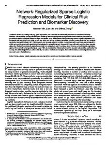
90.20±6.11 140

Fig.1. Sample images of one person on FERET face database

(a) (b) Fig.2. (a) The recognition rate versus the parameters  and  on the FERET face database. (b) The recognition rate versus the parameters  on the FERET, ORL, Yale, AR, Char74K_15 database, respectively. [4], the

L1 -norm

based dimensionality reduction methods, i.e.

Principal Component Analysis based on L1 -norm maximization (PCA-L1) [23], Linear Discriminant Analysis based on L1 -norm maximization (LDA-L1) [6] and Outlier-resisting graph embedding (LPP-L1) [7], the -norm regularization method (i.e.

L 2 ,1

L 2 ,1

-norm regularized

discriminative feature selection for unsupervised learning (UDFS) [31]), the nonlinear kernel-based method (KPCA) and the classical sparse learning method (i.e. robust face recognition via sparse representation (SRC-L1LS) [25]) . The Yale face database was used to evaluate the performance of GRR while there are variations in facial expression and lighting conditions. The AR database was used to explore the robustness of GRR in frontal views of faces with variational facial expressions, illumination and occlusions. The FERET and ORL databases were used to explore robustness of GRR with the variations of face images in facial expression and pose. Besides, the Char74K_15 database was used to test the performance of GRR in the English character images with excessive occlusion, low resolution or noise. The LFW database was used to evaluate the effectiveness of the proposed GRR and other competing methods based on deep learning situation.

In addition, the AR database was also used to test the robustness of the proposed GRR against the compared methods in three challenging situations (when training images are with random block corruption, disguise and illumination variation). A. Experiments on FERET face database The FERET face database is a result of the FERET program, which was sponsored by the USD department of Defense through the DARPA Program [37]. It has become a standard database for testing and evaluating state-of-the-art face recognition algorithms. The proposed method was tested on a subset of the FERET database. This subset included 1,400 images of 200 individuals (each individual has seven images) and involved variations in facial expression, illumination, and pose. In the experiment, the facial portion of each original image was automatically cropped based on the location of the eyes, and the cropped images were resized to 40×40 pixels. The sample images of one person are shown in Fig.1. Experimental setting: The performance of the feature selection methods (i.e. the proposed GRR and SPCA, LPP, RR, PCA-L1, LDA-L1, LPP-L1, UDFS, SRC-L1LS, KPCA) are measured by the recognition rate with selected features on the testing data set. PCA was first used as the pre-processing to reduce the dimensionality of the original data. The experiments were independently performed 10 times on the six databases. The nearest neighbor classifier is used for

1051-8215 (c) 2018 IEEE. Translations and content mining are permitted for academic research only. Personal use is also permitted, but republication/redistribution requires IEEE permission. See http://www.ieee.org/publications_standards/publications/rights/index.html for more information.

This article has been accepted for publication in a future issue of this journal, but has not been fully edited. Content may change prior to final publication. Citation information: DOI 10.1109/TCSVT.2018.2812802, IEEE Transactions on Circuits and Systems for Video Technology

8 TABLE III THE PERFORMANCE (RECOGNITION RATE, STANDARD DEVIATION AND DIMENSION) OF DIFFERENT METHODS ON THE ORL FACE DATABASE Training samples 3

4

5

SPCA

LPP

RR

PCA-L1

LDA-L1

LPP-L1

UDFS

KPCA

SRC-L1LS

GRR

89.46±1.76

76.82±1.72

87.32±1.88

89.46±1.62

71.46±3.59

83.50±3.10

90.14±1.88

85.64±2.91

90.89±1.79

99.64±0.00

95

60

40

95

15

100

55

95

100

25

92.79±1.73

85.79±2.30

90.87±1.75

92.83±1.88

82.00±1.74

88.00±2.49

92.92±1.64

90.58±2.16

93.42±1.79

99.58±0.00

100

90

40

100

25

90

60

95

75

35

94.80±1.46

90.00±1.59

92.50±1.37

94.70±1.41

87.30±2.74

90.85±1.67

95.00±1.56

92.55±2.54

95.10±1.73

100.00±0.00

55

65

40

85

50

100

60

95

60

10

Fig.3. Sample images of one person on ORL face database

(a) (b) Fig.4. (a) The recognition rates (%) versus the dimensions of different methods on the FERET face database. (b) The recognition rates (%) versus the dimensions of different methods on the ORL face database. classification. The average recognition rates and the corresponding dimensions and the standard deviations of each method were listed on the tables. Besides, the comparison results were also shown in the figures when several images of each individual were randomly selected for training while the remaining images were used for testing. The real dimension used in the experiment is the same with the number marked on the horizontal axis on the six data sets and all the images are cropped and aligned automatically. Usually, the initial value of the proposed algorithm has little effect on its performance, therefore the variables in GRR are randomly initialized in our experiments. Exploration of the performance of the parameters: Since the value of the three parameters  ,  and  affect the performance of the proposed GRR in some degree, thus we need to explore the optimal parameter values of GRR. For the other methods, since UDFS was introduced with the parameter lying on the area of [1 0  3 ,1 0 3 ] , then we used this area for UDFS to perform feature selection and presented the corresponding experimental results. The parameters of other methods were selected according to the related introduction in the original paper. In FERET database, we first analyze the optimal values of  ,  ,  and then use the values to obtain the best

performance for GRR. Table II shows the best average recognition rates, the corresponding dimensions and the standard deviations of different methods with different dimensions form 5 to 150 based on 10 times experiments. Fig. 2 (a) shows the recognition rates when the two parameters  and  change from 1 0  9 to 1 0 9 . Fig. 2 (b) presents the performance of the parameters  varies in the area of 9 9 [1 0 , 1 0 ] on all databases. It is obvious that, the value of  does not affect the performance when it lies in the area of 9 0 9 0 [1 0 , 1 0 ] . For simplicity, we choose   [1 0 , 1 0 ] in all experiments. Fig. 4 (a) shows the average recognition rates versus various dimensions of different methods when 6 images were selected for the training while the remaining images were used for testing. From the result showed in Fig. 2 (a), we obtain the optimal and are area for parameters   and [1 0  8 ,1 0  7 ,1 0  6 ,1 0  5 ,1 0  4 ] respectively. Namely, GRR obtains the best performance when the two parameters lie on these areas. Otherwise, other parameter values would cause the large decline of the face recognition rate of GRR. Table II shows that SRC-L1LS and GRR perform better than other methods. Fig. 4 (a) indicates when 6 images of each person are used for training, GRR [1 0

11

,1 0

10

,1 0

9

,1 0

8

,1 0

7

]

1051-8215 (c) 2018 IEEE. Translations and content mining are permitted for academic research only. Personal use is also permitted, but republication/redistribution requires IEEE permission. See http://www.ieee.org/publications_standards/publications/rights/index.html for more information.

This article has been accepted for publication in a future issue of this journal, but has not been fully edited. Content may change prior to final publication. Citation information: DOI 10.1109/TCSVT.2018.2812802, IEEE Transactions on Circuits and Systems for Video Technology

9 TABLE IV THE PERFORMANCE (RECOGNITION RATE, STANDARD DEVIATION AND DIMENSION) OF DIFFERENT METHODS ON THE YALE FACE DATABASE Training samples 4

5

6

SPCA

LPP

RR

PCA-L1

LDA-L1

LPP-L1

UDFS

KPCA

SRC-L1LS

GRR

92.95±4.00

86.86±4.38

91.43±4.60

92.67±3.79

82.67±7.25

60.67±6.91

92.10±4.29

91.90±3.98

97.24±1.57

97.14±0.00

25

38

15

36

38

6

35

39

8

13

93.00±4.29

89.89±3.56

93.00±4.91

93.22±4.66

83.44±7.98

64.00±8.20

92.67±4.87

92.56±5.08

97.67±1.33

98.89±0.00

30

27

15

26

28

7

36

39

7

12

94.13±4.83

94.13±4.09

94.67±5.01

94.13±5.16

84.53±7.03

85.73±9.80

92.93±5.79

93.33±5.50

97.47±2.33

100.00±0.00

23

31

15

20

23

36

37

39

8

8

Fig.5. Sample images of one person on Yale face database

(a) (b) Fig.6. (a) The recognition rates (%) versus the dimensions of different methods on the Yale face database. (b) The recognition rates (%) versus the dimensions of different methods on the AR face database. gives full play to its advantages and outperforms other methods with about 15.75% to 41.05% of the recognition rate. Moreover, GRR keeps going up smoothly and quickly achieves the best performance for feature selection. B. Experiments on ORL face database The ORL dataset consists of 10 face images from 40 subjects for a total of 400 images, with some variation in pose, facial expression and details. The resolution of the images is 112×92, with 256 gray-levels. Before the experiments, we scale the pixel gray level to the range [0, 1]. Fig. 3 depicts some sample images of a typical subset in the ORL dataset. In this experiment, l ( l  3, 4 , 5 ) images of each individual were randomly selected for training, and the rest of the images in the data set were used for testing. The optimal areas of parameter  and  were set in [1 0 6 ,1 0 7 ,1 0 8 ] and 5

4

3

2

[1 0 ,1 0 ,1 0 ,1 0 ] respectively. Fig. 4 (b) shows the average testing recognition rates. Table III listed the performance of different methods. It is obvious that GRR outperforms other methods again.

C. Experiments on Yale face database The Yale face database [43] was constructed at the Yale Center

for Computational Vision and Control. It contains 165 grayscale images of 15 individuals. The images demonstrate variations in lighting condition (left-light, center-light, right-light), facial expression (normal, happy, sad, sleepy, surprised, and wink), and with/without glasses. Fig. 5 shows the sample images from this database. In this experiment, l ( l  4 , 5, 6 ) images of each individual were randomly selected for training, and the rest of the images in the data set were used for testing. The optimal areas of parameter  and  were [1 0 7 ,1 0 8 ,1 0 9 ] and [1 0  7 ,1 0  6 ] , respectively. The performances of different methods are shown in Table IV. Fig. 6 (a) shows the average testing recognition rates when 6 images of each people were used for training. It clearly indicates that GRR obtains outstanding results. D. Experiments on AR face database The AR face database [38] contains over 4,000 color face images of 126 people (70 men and 56 women), including frontal views of faces with different facial expressions, lighting conditions, and occlusions. The pictures of 120 individuals (65 men and 55 women) were selected and divided into two sessions (separated by two weeks) and each session contains 13 color images. 20 images of these 120 individuals were selected

1051-8215 (c) 2018 IEEE. Translations and content mining are permitted for academic research only. Personal use is also permitted, but republication/redistribution requires IEEE permission. See http://www.ieee.org/publications_standards/publications/rights/index.html for more information.

This article has been accepted for publication in a future issue of this journal, but has not been fully edited. Content may change prior to final publication. Citation information: DOI 10.1109/TCSVT.2018.2812802, IEEE Transactions on Circuits and Systems for Video Technology

10 TABLE V THE PERFORMANCE (RECOGNITION RATE, STANDARD DEVIATION AND DIMENSION) OF DIFFERENT METHODS ON THE AR FACE DATABASE Training samples 4

5

6

SPCA

LPP

RR

PCA-L1

LDA-L1

LPP-L1

UDFS

KPCA

SRC-L1LS

GRR

81.92±4.73

86.90±4.97

75.67±6.61

81.93±4.74

51.20±11.94

57.48±11.40

81.93±4.79

81.85±6.12

87.75±2.37

92.21±4.03

150

150

105

150

20

145

150

145

150

110

84.62±4.07

89.83±3.84

81.49±4.62

84.62±4.02

54.23±9.22

59.72±8.32

84.62±4.04

86.07±6.85

89.08±2.87

93.47±3.32

150

150

105

150

55

150

150

145

150

75

85.08±4.89

91.60±3.65

83.95±4.44

85.08±4.93

58.56±7.47

58.83±8.33

85.08±4.89

86.72±4.20

89.62±3.13

93.87±3.00

150

150

105

150

45

150

150

140

150

80

(a)

(b) Fig.7. (a) The sample images of one person form the AR face database. (b) The sample images with block noise of one person in our experiment on the AR face database. and used in our experiments. The face portion of each image was manually cropped and then normalized to 50×40 pixels. The sample images of one person are shown in Fig. 7 (a). These images vary as follows: neutral expression, smiling, angry, screaming, left light on, right light on, all sides light on, wearing sun glasses, wearing sun glasses and left light on, wearing sun glasses and right light on. In this experiment, we randomly selected l ( l  4 , 5, 6 ) images of each individual for training, and the rest of the images in the data set were used for testing. The optimal areas of parameter  and  were in [1 0 7 ,1 0 8 ,1 0 9 ,1 0 1 0 ] and 2

1

respectively. Fig. 6 (b) shows the average testing recognition rates with 4 images of each object used as training set. Table V lists the performance of different methods. We can know from both Fig. 6 (b) and Table V that GRR outperforms the other methods. [1 0

,1 0

]

E. Experiments on Char74K_15 database The character images of the Char74K dataset [39] are mostly photographed from sign boards, hoardings and advertisements and a few images of products are in supermarkets and shops. Fig. 8. (a) depicts sample images of English scene characters from Char74k. As for the Char74K dataset, we only use the English character images cropped from the natural scene images. The English dataset has 12503 characters, of which 4798 were labeled as bad images due to excessive occlusion, low resolution or noise. It contains 62 character classes. A small subset with a standard partition is used in our experiments, i.e. Char74K-15, which contains 15 training samples per class and 15 test samples per class.

The optimal areas of 1

2

3

4

5



and



are

1

2

3

4

5

[1 0 ,1 0 ,1 0 ,1 0 ,1 0 ]

,

respectively. Fig.8 (b) demonstrates the average testing recognition rates versus the dimensions of different methods while Table VI shows the best average recognition rates and the corresponding dimensions and the standard deviations of each method. From the result, we can find that in this dataset, GRR outperforms other methods again. [1 0

,1 0

,1 0

,1 0

,1 0

]

F.

Robustness evaluation on AR face database To evaluate the performance of the proposed GRR and other compared methods in the case when there are various noises corrupted in the images, we conducted series of experiment including random block corruption and disguise as well as illumination variation. 1) Images With Random block Corruption To evaluate the robustness of the proposed GRR, the noise was added in the face images in our experiments and the samples image with block noise of one person are shown in Fig.7 (b). Table VII lists the best average recognition rates, the corresponding dimensions and the standard deviations of different methods based on 10 times experiments on AR database with block size 5*5, 10*10, 15*15, respectively. Fig.9 (a) shows the average recognition rates versus the dimensions of different methods in the case when 4 images of each individual were randomly selected for training from the images that are corrupted by a block size 10*10. All of the results prove the robustness and effectiveness of the proposed GRR. 2) Images With Disguise

1051-8215 (c) 2018 IEEE. Translations and content mining are permitted for academic research only. Personal use is also permitted, but republication/redistribution requires IEEE permission. See http://www.ieee.org/publications_standards/publications/rights/index.html for more information.

This article has been accepted for publication in a future issue of this journal, but has not been fully edited. Content may change prior to final publication. Citation information: DOI 10.1109/TCSVT.2018.2812802, IEEE Transactions on Circuits and Systems for Video Technology

11

TABLE VI THE PERFORMANCE (RECOGNITION RATE, STANDARD DEVIATION AND DIMENSION) OF DIFFERENT METHODS ON THE CHAR74K_15 FACE DATABASE Method Recognition rate

SPCA

LPP

RR

PCA-L1

LDA-L1

LPP-L1

UDFS

KPCA

SRC-L1LS

GRR

59.03±0.00

60.22±0.00

37.42±0.00

58.68±0.14

50.45±0.61

47.91±1.01

18.71±0.00

59.14±0.00

65.27±0.00

65.41±0.36

64

48

62

66

48

80

76

70

62

72

(a)

(b)

Fig.8. (a) Sample images of English scene characters from Char74k. (b) The recognition rates (%) versus the dimensions of different methods on the Char74K_15 face databases.

(a) (b) Fig.9. (a) The recognition rates (%) versus the dimensions of different methods on the AR face databases with noise. (b) An example of the convergence curve of GRR. To investigate the proposed GRR and other compared methods in the case when training set is corrupted by varying percentage of occlusion in face images, two protocols are conducted as similar in [40] [41]. That is, occlusion in training set due to (1) sunglasses, (2) scarf, respectively. Note that scarf accounts for occlusion of about 40% of each face image while the occlusion of sunglasses amounts to about 20%. Fig.10. shows the sample image of session 1 on AR database in our experiment. Sunglasses: For each individual, n c neutral images and no 

{0, 1, 2, 3} occluded image(s) from Session 1 are used

for training, where n c  n o  7 . Session 2 including 7 neutral images plus 3 occluded image (sunglasses) are used for testing.

Scarf: The setup of training set and testing set are the same with sunglasses case except using scarf instead of sunglasses as occlusion of the images. The results of the above two occlusion cases are presented in table VIII. It is obvious that the proposed GRR and SRC always perform better than other methods in these situations. For the sunglasses case, SRC performs a little better than GRR as a whole, yet GRR definitely outperforms SRC under the scarf case. The reason is as follow. SRC assumes the testing image is approximately reconstructed by the training image. However, if the training set include few or even no occluded images, the reconstructed error as classification criteria is not so effective since it varies in large range. In these two occluded cases, especially the scarf case (since the occlusion percentage is much higher), SRC generates large reconstruction errors which bring negative impact on face

1051-8215 (c) 2018 IEEE. Translations and content mining are permitted for academic research only. Personal use is also permitted, but republication/redistribution requires IEEE permission. See http://www.ieee.org/publications_standards/publications/rights/index.html for more information.

This article has been accepted for publication in a future issue of this journal, but has not been fully edited. Content may change prior to final publication. Citation information: DOI 10.1109/TCSVT.2018.2812802, IEEE Transactions on Circuits and Systems for Video Technology

12 TABLE VII THE PERFORMANCE (RECOGNITION RATE, STANDARD DEVIATION AND DIMENSION) OF DIFFERENT METHODS ON THE AR FACE DATABASE WITH NOISE

Block size

5*5

10*10

15*15

Training samples

SPCA

LPP

RR

PCA-L1

LDA-L1

LPP-L1

UDFS

KPCA

SRC-L1LS

GRR

4

80.47±4.73 150

83.46±5.46 150

73.70±6.16 105

80.22±4.97 150

47.41±10.88 40

53.81±10.58 150

80.64±4.86 150

83.50±5.45 145

86.12±2.40 150

90.83±4.37 120

5

83.39±3.91 150

87.49±4.01 150

79.19±4.20 105

83.28±4.10 150

51.38±8.04 50

58.78±7.80 150

83.38±3.95 145

83.08±5.19 145

87.65±2.92 150

92.42±4.00 110

6

83.76±4.69 150

89.47±4.42 150

81.82±4.21 105

83.94±4.78 150

55.32±8.34 50

58.21±6.31 150

84.10±4.65 135

86.55±4.61 145

88.26±3.22 150

93.01±3.52 120

4

69.74±5.45 150

75.78±6.52 150

60.64±4.93 100

70.85±5.15 145

35.56±8.43 35

45.52±10.32 150

69.92±5.44 150

67.89±7.70 145

74.96±2.65 150

85.73±4.82 120

5

73.11±3.55 150

80.45±5.78 150

66.28±3.24 100

74.09±3.90 150

41.16±4.72 50

48.97±6.27 145

73.20±3.83 150

69.63±5.80 145

77.32±2.79 150

88.55±3.65 130

6

73.99±4.21 145

82.91±6.11 150

69.21±3.77 105

75.11±4.43 150

44.76±5.33 75

49.81±5.83 150

74.14±4.59 145

72.12±6.31 145

78.36±2.83 150

89.36±3.36 115

4

50.82±4.17 150

56.36±5.86 150

45.95±3.59 105

50.66±4.80 150

25.92±5.18 35

32.34±6.46 150

51.06±4.24 135

50.63±3.61 145

55.79±2.45 150

73.34±5.29 120

5

54.26±2.83 150

61.83±6.55 150

51.97±2.22 105

54.26±3.46 150

30.11±3.99 40

34.39±4.06 150

54.31±2.86 140

56.83±2.90 140

58.76±2.36 150

78.22±2.66 120

6

56.24±2.82 145

65.81±6.08 150

55.96±2.96 105

56.08±3.50 150

32.36±5.43 55

36.05±4.92 150

56.24±2.85 150

58.45±3.48 140

60.48±2.82 150

80.13±2.99 120

Fig.10 Example images from Session 1 of the AR database. recognition task. On the contrary, the proposed GRR can guarantee the robustness by designing a more compact and effective model. On one hand, it utilizes L 2 ,1 -norm minimization instead of L 2 -norm to alleviate the sensitiveness to outliers. On the other hand, it uses the elastic factor h to avoid the overfitting problem in this case. 3) Images With Illumination variation In this part, the first 7 images of each person on the AR database are used to form the training set and testing set. For each individual, the first 4 images varying on facial expression plus n il  {0, 1, 2, 3} image(s) varying on illumination in Session 1 are used to form the training set and the images in Session 2 are used as the testing set. That is, n n i  {4, 5, 6, 7} images of each person are used for training. Table IX shows the corresponding experimental results. It is obvious that SRC and GRR are comparative and they always outperform other compared methods. Although GRR seems to be a little inferior to SRC at first, it finally catches up and even outperforms SRC. G.

Reconstruction and Subspace Learning This subsection further performs a set of experiments to explore the learned subspace properties of the proposed GRR and some classical methods, i.e. PCA, RPCA, RR and LPP. In this part, we consider two versions of experiments. For the first version, 7 neutral images of each individual from AR database are trained by LPP, RR, PCA, RPCA and GRR, respectively and the corresponding results are plotted as

images. Fig.11 (a) shows the original image of one person in our experiment. Fig.11 (b)-(d) show reconstruction images obtained by RPCA, PCA, GRR, respectively. Note that for RPCA, the learned low-rank approximation is presented in this experiment. For PCA, 50 principle components are used for reconstruction. To explore the properties of the subspaces learned by GRR and other subspace learning methods (i.e. LPP, RR, PCA), we also present the images of the first 2 projections learned by these methods. Fig.11 (e)-(h) show the first 2 projections of the subspace obtained by LPP, RR, PCA, GRR, respectively. In the second version, all the training images are corrupted by random block noise with 50*50 pixels and the results are shown in Fig. 12. According to these experimental results, we have the following interesting conclusion: RPCA is good at recovering low-rank components of the original data. It can get rid of the corrupted noise in some degree, which can be seen from Fig.12 (b). PCA is an effective method for reconstructing the original images. However, GRR does not tend to reconstruct the original images since it focus on discriminant information instead of reconstruction. That is, GRR finds the most discriminative projections to obtain an optimal subspace for efficient feature selection or extraction. As it can be seen from Fig.12 (d) and Fig.12 (h), the block noise on the face image is not evident. On the contrary, Fig.12 (g) shows that the block noise on PCA-based images is quite obvious. This indicates that GRR can avoid the noise impact more effectively than PCA. Both

1051-8215 (c) 2018 IEEE. Translations and content mining are permitted for academic research only. Personal use is also permitted, but republication/redistribution requires IEEE permission. See http://www.ieee.org/publications_standards/publications/rights/index.html for more information.

This article has been accepted for publication in a future issue of this journal, but has not been fully edited. Content may change prior to final publication. Citation information: DOI 10.1109/TCSVT.2018.2812802, IEEE Transactions on Circuits and Systems for Video Technology

13 TABLE VIII COMPARISONS (RECOGNITION RATE STANDARD DEVIATION AND DIMNSION) WTH DIFFEENT PERCENTAGES OF OCCLUDED IMAGES ( n o / 7 ) PRESENTED IN THE TRAINING SET. THE FEATURE DIMENSION IS SET AS 150 FOR ALL METHODS.

Method

Sunglasses

Scarf

Sunglasses

0% = 0/7

Scarf

14.29% = 1/7

Sunglasses

Scarf

28.57% = 2/7

Sunglasses

Scarf

42.86% = 3/7

SPCA

54.70±0.00 145

50.90±0.00 145

55.59±2.76 150

51.18±2.20 150

57.03±3.27 150

49.69±2.44 150

56.63±2.51 150

48.50±2.97 150

LPP

55.00±0.00 140

51.60±0.00 140

58.35±1.86 150

50.66±1.99 150

59.19±2.02 150

51.32±1.74 150

58.71±2.55 150

47.36±2.30 150

RR

51.40±0.00 75

44.50±0.00 100

56.91±1.01 70

49.99±1.64 100

57.52±1.17 70

51.32±2.47 100

57.56±0.41 70

52.85±0.81 100

PCA-L1

54.83±0.11 145

50.94±0.13 145

55.59±2.75 150

51.24±2.22 150

57.10±3.30 150

49.71±2.45 150

56.64±2.58 150

48.52±2.94 150

LDA-L1

34.87±0.79 110

33.49±0.70 75

34.85±3.22 80

33.53±2.03 90

38.15±2.36 90

31.34±3.05 110

38.95±2.57 75

29.64±2.90 95

LPP-L1

7.61±0.85 5

7.39±1.19 5

8.74±2.55 5

9.28±1.44 10

9.20±3.37 5

8.84±0.48 10

10.02±1.91 5

7.71±0.90 5

UDFS

55.00±0.00 125

51.10±0.00 140

55.69±2.77 135

51.38±2.20 125

57.13±3.34 130

49.87±2.51 105

56.74±2.52 135

48.99±3.10 110

KPCA

56.54±1.01 145

51.14±1.07 145

57.56±3.28 145

52.93±3.35 145

58.42±4.12 145

53.42±2.77 145

59.10±2.83 145

51.74±4.39 145

SRC_L1LS

59.40±0.00 150

51.90±0.00 150

60.00±1.73 150

54.67±1.50 150

60.85±1.87 150

55.28±1.83 150

60.01±1.71 150

53.67±1.24 150

GRR

57.24±0.58 150

52.65±0.53 145

58.24±2.51 145

56.30±1.59 145

60.33±2.99 150

57.26±2.49 140

61.48±2.96 150

55.14±3.42 145

TABLE IX THE PERFORMANCE (RECOGNITION RATE, STANDARD DEVIATION AND DIMENSION) OF DIFFERENT METHODS ON AR DATABASE WITH VARIOUS ILLUMINATION. THE FEATURE DIMENSION IS SET AS 150 FOR ALL METHODS. Illumination

Illumination

Illumination

Illumination

0% = 0/4

20% = 1/5

33.33% = 2/6

42.86% = 3/7

SPCA

40.86±0.00 145

52.19±0.48 150

61.89±0.87 145

70.57±0.00 145

LPP

44.43±0.00 130

54.51±3.14 145

65.14±3.62 145

68.71±0.00 140

RR

44.29±0.00 65

52.77±1.55 75

61.27±0.92 70

64.14±0.00 70

PCA-L1

40.86±0.10 150

52.27±0.46 145

61.89±0.77 145

70.59±0.12 145

LDA-L1

19.61±0.88 85

29.81±0.98 45

35.09±2.04 70

42.89±1.71 85

LPP-L1

13.26±0.78 5

10.86±1.24 5

37.53±3.02 150

43.77±2.46 150

UDFS

41.14±0.00 140

52.51±0.52 140

62.29±0.60 130

70.71±0.00 125

KPCA

45.14±3.76 145

53.41±2.64 145

64.47±4.07 145

70.54±1.42 145

SRC_L1LS

53.71±0.00 150

60.71±2.39 150

65.34±0.44 150

71.14±0.00 150

GRR

44.83±0.71 85

57.86±0.85 145

65.93±0.72 135

73.29±0.30 125

Method

LPP and RR can obtain the face-like images, but LPP’s projections are affected seriously by the block noise. H.

Experiments on LFW database based on deep learning The LFW database [42] is a very challenging dataset which contains images of 5,749 subjects in the uncontrolled environment. The LFW-a dataset is the aligned version of LFW after performing the face alignment. In our experiment, 4324 images of 158 subjects (each subject has more than 10

images) are selected from LFW-a dataset. Note that all images are aligned as well as cropped and resized to 112*96 pixels. Fig.13 shows the sample images in our experiment. The LFW database were used to evaluate the performance of the proposed GRR and other competing methods based on the deep learning techniques. Similar to [43], the deep convolutional neural network (CNN) was used as the feature extractor to obtain the deep features of all samples (the number of the features is 1024). After the deep features were obtained,

1051-8215 (c) 2018 IEEE. Translations and content mining are permitted for academic research only. Personal use is also permitted, but republication/redistribution requires IEEE permission. See http://www.ieee.org/publications_standards/publications/rights/index.html for more information.

This article has been accepted for publication in a future issue of this journal, but has not been fully edited. Content may change prior to final publication. Citation information: DOI 10.1109/TCSVT.2018.2812802, IEEE Transactions on Circuits and Systems for Video Technology

14

(a) (b) (c) (d) (e) (f) (g) (h) Fig.11. (a) is original sample images, (b), (c), (d) is reconstruction images obtained by RPCA, PCA, GRR, respectively; (e), (f), (g), (h) is 2 images of the first 2 projections from subspace obtained by LPP, RR, PCA, GRR, respectively.

(a) (b) (c) (d) (e) (f) (g) (h) Fig.12. (a) is corrupted images by block noise with size 50*50, (b), (c), (d) is reconstruction images obtained by RPCA, PCA, GRR, respectively; (e), (f), (g), (h) is 2 images of the first 2 projections from subspace obtained by LPP, RR, PCA, GRR, respectively.

Fig.13 Example images from LFW database TABLE X THE PERFORMANCE OF DIFFERENT METHODS ON THE LFW FACE DATABASE Training samples

SPCA

LPP

RR

PCA-L1

LDA-L1

LPP-L1

UDFS

KPCA

SRC-L1LS

GRR

4

95.29

64.68

93.40

95.35

61.16

86.29

94.86

95.83

94.53

95.88

5

95.42

72.38

94.04

95.59

69.20

90.78

94.93

96.13

95.45

96.87

6

95.79

78.94

94.48

95.82

76.82

87.80

95.34

96.49

95.96

97.01

7

95.82

64.14

94.80

95.85

83.19

87.60

95.38

96.48

96.10

97.58

we further used the subspace learning methods (i.e. SPCA, LPP, RR, PCA-L1, LDA-L1, LPP-L1, UDFS, KPCA, SRC-L1LS and the proposed GRR) to perform feature extraction, and then the nearest neighbor classifier was used for classification. In this experiment, we randomly selected l ( l  4 , 5, 6 , 7 ) images of each subject to form the gallery set and the rest are used as probe set. The optimal areas of parameter  and  are [1 0 7 ,1 0 8 ,1 0 9 ,1 0 1 0 ] and [1 0  2 ,1 0  1 ] , respectively. The best recognitions rates of deep feature plus the subspace learning methods are shown in Table X. The results indicate the performance of the proposed GRR is still better than other methods. Fig.9 (b) shows an example of the convergence curve of GRR. I. Experimental results and discussions From the experimental results listed in Tables and the figures presented in previous subsections, we can draw the following interesting points: 1. All the experimental results indicate that GRR outperforms the other methods. This is because GRR integrates multiple robust factors and locality based on the combination of RR, LPP and the L 2 ,1 -norm minimization. Thus, with these advantages, GRR is capable to outperform the conventional RR and LPP as well as the L1 -norm based methods. 2. From Fig. 4 (b), 6 and 8 (b), we can know that the projection learned from the traditional ridge regression RR is no more than the number of the class in training data while

GRR can learn any number of projections and preserve high and stable recognition rate. Especially, Table VI showed that when RR obtained the best recognition rate on the dimension of 62 (i.e. the number of class), GRR broke out this number and obtained the best recognition rate on the dimension of 72. This is because RR has the small-class problem which makes the number of the projections limited by the number of the class in training data. However, GRR can break out this limitation to obtain enough projections to obtain high recognition rate for face recognition, character recognition or other practical applications. 3. GRR obtains quite good performance on these databases when there are variations on pose and face expressions. The reason is that GRR not only uses the L 2 ,1 - norm on both the loss function and regularization term, but also takes the local geometric structure into consideration. These techniques guarantee the joint sparsity and local information for GRR to obtain effective features to increase the recognition rates. 4. As demonstrated in Subsection IV-F, when training images are with random block corruption, disguise or illumination variation, GRR still outperforms the other methods and obtains the better recognition rate in most cases. Comparing with the other methods, another potential reason for the good performance of GRR is that the elastic factor h on the loss function is capable to decrease the negative influence caused by the block subtraction, noise or disguise.

1051-8215 (c) 2018 IEEE. Translations and content mining are permitted for academic research only. Personal use is also permitted, but republication/redistribution requires IEEE permission. See http://www.ieee.org/publications_standards/publications/rights/index.html for more information.

This article has been accepted for publication in a future issue of this journal, but has not been fully edited. Content may change prior to final publication. Citation information: DOI 10.1109/TCSVT.2018.2812802, IEEE Transactions on Circuits and Systems for Video Technology

15 5. In most cases, the

L 2 ,1 -norm based

methods (i.e. GRR and

UDFS) obtain the better performance than the L1 -norm based methods (i.e. PCA-L1, LPP-L1, LDA-L1). The main reason is that using L 2 ,1 -norm on the regularization term can improve the recognition rates since it performs the joint sparse feature selection in extraction step. 6. The state-of-the-art recognition rate on FERET, ORL, Yale, AR and LFW database is 71.25%, 98.90%, 98.80%, 91.23% and 53.39% when 4, 5, 5, 5, 6 images of each subject are used as training, respectively [44] [45] [46]. The newest maximum recognition rate on Char74K_15 is 67.00% [47]. From the experimental results, we can find that the recognition rates of the proposed GRR are higher than the state-of-the-art recognition rates on ORL, Yale and AR database and also competitive on other databases. This indicates that GRR is an effective method for feature extraction and classification. V.

CONCLUSION

Motivated by the robustness and

L 2 ,1 -norm

minimization on

loss function and regularization term, a novel method called Generalized Robust Regression (GRR) is proposed for jointly sparse subspace learning. GRR integrates the advantages of locality preserving projections and L 2 ,1 -norm minimization to select informative features and at the same time guarantee the robustness in the learning procedure by introducing an elastic factor. GRR also breaks out the small-class problem which exists in the traditional ridge regression or its derivatives so as to obtain enough projections to perform efficient feature extraction or selection. To optimize the problem of GRR, an iterative algorithm is proposed and the convergence is also proved in this paper. Moreover, we also analyze the computational complexity of the proposed algorithm. The favorable performance of GRR on six well-known databases indicates that GRR outperforms the conventional Sparse Principal Component Analysis (SPCA), Locality Preserving Projections (LPP), the traditional Ridge regression (RR), the L1 -norm based methods PCA-L1, LDA-L1, LPP-L1, the L 2 ,1 -norm regularized discriminative feature selection method UDFS, the nonlinear kernel-based method (KPCA) and the classical sparse learning method (i.e. SRC-L1LS). Since the proposed GRR is an iteration algorithm, its computational complexity is more than the traditional LPP-based methods. Also, the case of imbalanced data is not taken into consideration in this paper. Therefore, how to reduce the computation cost as well as how to extend the regression method to deal with the imbalanced data is an interesting research in the near future. REFERENCE [1] S. Xiang, F. Nie, G. Meng, C. Pan, and C. Zhang, “Discriminative least squares regression for multiclass classification and feature selection,” IEEE Trans. Neural Networks Learn. Syst., vol. 23, no. 11, pp. 1738–1754, 2012. [2] Y. Xu, D. Zhang, J. Yang, and J. Yang, “A two-phase test sample sparse representation method for use with face recognition,” IEEE Trans. Circuits Syst. Video Technol., vol. 21, no. 9, pp. 1255 – 1262, 2011.

[3] Y. Huang, D. Xu, and F. Nie, “Patch distribution compatible semisupervised dimension reduction for face and human gait recognition,” IEEE Trans. Circuits Syst. Video Technol., vol. 22, no. 3, pp. 479–488, 2012. [4] N. R. Draper and R. C. Van Nostrand, “Ridge regression,” Quality, vol. 21, no. 4, pp. 451–466, 2011. [5] H. Zou, T. Hastie, and R. Tibshirani, “Sparse principal component analysis,” J. Comput. Graph. Stat., vol. 15, no. 2, pp. 1–30, 2004. [6] L. Maximization, “Linear Discriminant Analysis based on L1-norm maximization,” IEEE Trans. Image Process., vol. 22, no. 8, pp. 3018– 3027, 2013. [7] Y. Pang and Y. Yuan, “Outlier-resisting graph embedding,” Neurocomputing, vol. 73, no. 4–6, pp. 968–974, 2010. [8] Y. Xu, Z. Zhang, G. Lu, and J. Yang, “Approximately symmetrical face images for image preprocessing in face recognition and sparse representation based classification,” Pattern Recognit., vol. 54, pp. 68–82, 2016. [9] X. Huang, Z. Lei, M. Fan, X. Wang, and S. Z. Li, “Regularized discriminative spectral regression method for heterogeneous face matching,” IEEE Trans. Image Process., vol. 22, no. 1, pp. 353–362, 2013. [10] S. T. Roweis and L. K. Saul, “Nonlinear dimensionality reduction by locally linear embedding.,” Science, vol. 290, no. 5500, pp. 2323–2326, 2000. [11] M. Belkin and P. Niyogi, “Laplacian eigenmaps for dimensionality reduction and data representation,” Neural Comput., vol. 15, no. 6, pp. 1373–1396, 2003. [12] J. B. Tenenbaum, V. de Silva, and J. C. Langford, “A global geometric framework for nonlinear dimensionality reduction.,” Science, vol. 290, no. 5500, pp. 2319–23, 2000. [13] X. He and P. Niyogi, “Locality preserving projections,” Neural Inf. Process. Syst., vol. 16, no. 1, pp. 186–197, 2004. [14] X. He, S. Yan, Y. Hu, P. Niyogi, and H. J. Zhang, “Face recognition using Laplacianfaces,” IEEE Trans. Pattern Anal. Mach. Intell., vol. 27, no. 3, pp. 328–340, 2005. [15] Y. Pang, L. Zhang, Z. Liu, N. Yu, and H. Li, “Neighborhood preserving projections (NPP): a novel linear dimension reduction method,” Adv. Intell. Comput., no. 3644, pp. 117–125, 2005. [16] Xiaofei He, Deng Cai, Shuicheng Yan, and Hong-Jiang Zhang, “Neighborhood preserving embedding,” Tenth IEEE Int. Conf. Comput. Vis. Vol. 1, vol. 2, pp. 1208–1213, 2005. [17] H. Wang, Q. Tang, and W. Zheng, “L1-norm-based common spatial patterns,” IEEE Trans. Biomed. Eng., vol. 59, no. 3, pp. 653–662, 2012. [18] Y. Pang, X. Li, and Y. Yuan, “Robust tensor analysis with L1-norm,” IEEE Trans. Circuits Syst. Video Technol., vol. 20, no. 2, pp. 172–178, 2010. [19] E. J. Cand, X. Li, Y. Ma, and J. Wright, “Robust Principal Component Analysis ?,” J. Acm, vol. 58, no. 3, 2009. [20] Z. Lin and M. Chen, “The augmented lagrange multiplier method for exact recovery of corrupted low-rank matrices,” Math. Program., vol. 9, 2010. [21] Qifa Ke and T. Kanade, “Robust L1 norm factorization in the presence of outliers and missing data by alternative convex programming,” 2005 IEEE Comput. Soc. Conf. Comput. Vis. Pattern Recognit., vol. 1, pp. 739–746, 2005. [22] C. Ding, D. Zhou, X. He, and H. Zha, “R1-PCA: rotational invariant L1-norm principal component analysis for robust subspace factorization,” Proceedings of the 23rd international conference on Machine learning ICML ’06. pp. 281–288, 2006. [23] N. Kwak, “Principal component analysis based on L1-norm maximization,” IEEE Trans. Pattern Anal. Mach. Intell., vol. 30, no. 9, pp. 1672–1680, 2008. [24] X. Li, W. Hu, H. Wang, and Z. Zhang, “Linear discriminant analysis using rotational invariant L1-norm,” Neurocomputing, vol. 73, no. 13–15, pp. 2571–2579, 2010. [25] J. Wright, S. Member, A. Y. Yang, A. Ganesh, S. Member, and S. S. Sastry, “Robust face recognition via sparse representation,” IEEE Trans. Pattern Anal. Mach. Intell., vol. 31, no. 2, pp. 210–227, 2009. [26] L. Wang, H. Wu, and C. Pan, “Manifold regularized local sparse representation for face recognition,” IEEE Trans. Circuits Syst. Video Technol., vol. 25, no. 4, pp. 651–659, 2015. [27] B. Wohlberg, “Efficient algorithms for convolutional sparse representations,” Ieee Trans. Image Process., vol. 25, no. 1, pp. 301–315, 2016.

1051-8215 (c) 2018 IEEE. Translations and content mining are permitted for academic research only. Personal use is also permitted, but republication/redistribution requires IEEE permission. See http://www.ieee.org/publications_standards/publications/rights/index.html for more information.

This article has been accepted for publication in a future issue of this journal, but has not been fully edited. Content may change prior to final publication. Citation information: DOI 10.1109/TCSVT.2018.2812802, IEEE Transactions on Circuits and Systems for Video Technology

16 [28] F. Nie, H. Huang, X. Cai, and C. Ding, “Efficient and robust feature selection via joint L2,1-norms minimization,” Adv. Neural Inf. Process. Systens 23, pp. 1813–1821, 2010. [29] C. Hou, F. Nie, D. Yi, and Y. Wu, “Feature selection via joint embedding learning and sparse regression,” Int. Jt. Conf. Artif. Intell., pp. 1324–1329, 2011. [30] Q. Gu, Z. Li, and J. Han, “Joint feature selection and subspace learning,” in The 22nd International Joint Conference on Artificial Intelligence (IJCAI), 2011, vol. 55, pp. 1294–1299. [31] Y. Yang, H. T. Shen, Z. Ma, Z. Huang, and X. Zhou, “L21-norm regularized discriminative feature selection for unsupervised learning,” IJCAI Int. Jt. Conf. Artif. Intell., pp. 1589–1594, 2011. [32] V. Sindhwani and P. Niyogi, “Linear manifold regularization for large scale semi-supervised learning,” Present. Work. Learn. With Partial. Classif. Train. Data, Int. Conf. Mach. Learn. Bonn,Germany, pp. 80–83, 2005. [33] F. Nie, D. Xu, I. W. H. Tsang, and C. Zhang, “Flexible manifold embedding: a framework for semi-supervised and unsupervised dimension reduction,” IEEE Trans. Image Process., vol. 19, no. 7, pp. 1921–1932, 2010. [34] F. Zhong, J. Zhang, and D. Li, “Discriminant locality preserving projections based on L1-norm maximization,” IEEE Trans. Neural Networks Learn. Syst., vol. 25, no. 11, pp. 2065–2074, 2014. [35] W. Yu, X. Teng, and C. Liu, “Face recognition using discriminant locality preserving projections,” Image Vis. Comput., vol. 24, no. 3, pp. 239–248, 2006. [36] Y. Lu, Z. Lai, Y. Xu, X. Li, D. Zhang, and C. Yuan, “Low-rank preserving projections,” IEEE Trans. Cybern., vol. PP, no. 99, pp. 1–14, 2015. [37] P. J. Phillips, H. Moon, P. Rauss, S. A. Rizvi, S. Island, N. York, and S. Island, “The FERET evaluation methodology for face-recognition algorithms state university of new york at buffalo , amherst , NY 14260,” pp. 137–143, 1997. [38] A. A. Martinez and R. Benavente, “The AR face database,” CVC Tech. Rep. 24, 1998. [39] T. E. de Campos, B. R. Babu, and M. Varma, “Character recognition in natural images.,” Proc. Fourth Int. Conf. Comput. Vis. Theory Appl., pp. 273–280, 2009. [40] C. Wei, C. Chen, and Y. F. Wang, “Robust face recognition with structurally incoherent low-rank matrix decomposition,” IEEE Trans. Image Process., vol. 23, no. 8, pp. 3294–3307, 2014. [41] C. Georgakis, Y. Panagakis, and M. Pantic, “Discriminant Incoherent Component Analysis,” IEEE Trans. Image Process., vol. 25, no. 5, pp. 2021–2034, 2016. [42] G. B. Huang, M. Mattar, T. Berg, and E. Learned-miller, “Labeled Faces in the Wild : A Database for Studying Face Recognition in Unconstrained Environments,” Tech. Rep. 07-49, Univ. Massachusetts, Amherst ,2007. [43] Y. Wen, K. Zhang, Z. Li, and Y. Qiao, “A Discriminative Feature Learning Approach for Deep Face Recognition,” Eur. Conf. Comput. Vis., pp. 499–515, 2016. [44] A. Nazari, “A Constructive Genetic Algorithm for LBP in Face Recognition,” 3rd Int. Conf. Pattern Recognit. Image Anal., pp. 182–188, 2017. [45] T. Alobaidi and W. B. Mikhael, “Two-Step Feature Extraction in A Transform Domain for Face Recognition,” IEEE Comput. Commun. Work. Conf., pp. 1–4, 2017. [46] J. Liang, C. Chen, Y. Yi, and X. Xu, “Bilateral Two-Dimensional Neighborhood Preserving Discriminant Embedding for Face Recognition,” IEEE Access, vol. PP, no. 99, pp. 1–1, 2017. [47] Z. Zhang and Y. Xu, “Natural Scene Character Recognition Using Robust PCA and Sparse Representation,” 12th IAPR Int. Work. Doc. Anal. Syst., pp. 340–345, 2016.

Zhihui Lai received the B.S. degree in mathematics from South China Normal University, M.S. degree from Jinan University, and the Ph.D. degree in pattern recognition and intelligence system from the Nanjing University of Science and Technology, China, in 2002, 2007, and 2011, respectively. He has been a Research Associate, Post-Doctoral Fellow, and a Research Fellow with The Hong Kong Polytechnic University. He has authored over

60 scientific articles. His current research interests include face recognition, image processing, and content based image retrieval, pattern recognition, compressive sense, human vision modelization, and applications in the fields of intelligent robot research. He is currently an Associate Editor of International Journal of Machine Learning and Cybernetics.

Dongmei Mo received the B.S degree in Zhao Qing University and she is now pursuing the M.S degree in Shenzhen University. She is with the College of Computer Science and Software Engineering, Shenzhen University, Shenzhen 518060. Her current research interests include artificial intelligence and pattern recognition (e-mail: [email protected]).

Jiajun Wen received the Ph.D. degree in computer science and technology from Harbin Institute of Technology, China, in 2015. He has been a Research Associate with the Hong Kong Polytechnic University, Hong Kong, since 2013. He is currently a Postdoctoral Fellow with the College of Computer Science & Software Engineering, Shenzhen University, Shenzhen, China. His research interests include pattern recognition and video analysis.

Linlin Shen received the Ph.D. degree from the University of Nottingham, Nottingham, U.K., in 2005. He was a Research Fellow with Medical School, University of Nottingham, researching brain image processing of magnetic resonance imaging. He is currently a Professor and a Director with the Computer Vision Institute, College of Computer Science and Software Engineering, Shenzhen University, Shenzhen, China. His current research interests include Gabor wavelets, face/palmprint recognition, medical image processing, and hyperspectral image classification.

Wai Keung Wong received the Ph.D. degree from The Hong Kong Polytechnic University, Hung Hom, Kowloon, Hong Kong. He is currently a Professor with The Hong Kong Polytechnic University. He has authored or co-authored more than 100 papers in refereed journals and conferences, including the IEEE Transactions on Neural Networks and Learning Systems, the IEEE Transactions on Systems, Man, and Cybernetics-Part B: Cybernetics and the IEEE Transactions on Systems, Man, and Cybernetics-Part C: Applications and Reviews, Pattern Recognition, CHAOS, European Journal of Operational Research, Neural Networks, Applied Soft Computing, Information Science, Decision Support Systems, among others. His current research interests include pattern recognition and feature extraction.

1051-8215 (c) 2018 IEEE. Translations and content mining are permitted for academic research only. Personal use is also permitted, but republication/redistribution requires IEEE permission. See http://www.ieee.org/publications_standards/publications/rights/index.html for more information.