Sparse multiresolution stochastic approximation for uncertainty ...

93

Center for Turbulence Research Annual Research Briefs 2012

Sparse multiresolution stochastic approximation for uncertainty quantification By D. Schiavazzi, A. Doostan

AND

G. Iaccarino

1. Motivation and objectives Most physical systems are inevitably affected by uncertainties due to natural variabilities or incomplete knowledge about their governing laws. To achieve predictive computer simulations of such systems, a major task is, therefore, to study the impact of these uncertainties on response quantities of interest. Within the probabilistic framework, uncertainties may be represented in the form of random variables/processes. Several computational strategies may then be applied to propagate these uncertainties in order to obtain the statistics of quantities of interest. Monte Carlo (MC) sampling methods have been widely used for this purpose. Besides their generally slow convergence, they offer a blend of simplicity, robustness, and efficiency for high-dimensional problems. Recently, there has been an increasing interest in developing more efficient alternative numerical methods. Most notably, stochastic approximation schemes based on Wiener-Askey polynomial chaos expansions (Ghanem & Spanos 2003; Xiu & Karniadakis 2002) or interpolations on sparse grids (Xiu & Hesthaven 2006) have been applied successfully to a variety of problems with random inputs. For sufficiently smooth solutions, these methods achieve as high as exponential convergence rate in the mean-squares sense. For non-smooth responses such as those exhibiting sharp gradients or discontinuities, however, these methods may result in poor approximations. To address this shortcoming, various methodologies including adaptive multiresolution (Le Maıtre et al. 2004), multi-element (generalized) polynomial chaos (Wan & Karniadakis 2005), adaptive sparse grid collocation (Ma & Zabaras 2009), rational approximation (Chantrasmi et al. 2009), and simplex stochastic collocation (Witteveen & Iaccarino 2012), have been suggested in recent years. In this work, we present a multiresolution approach based on sparse multiwavelet expansions for uncertainty propagation. Unlike the work in Le Maıtre et al. (2004) where the multiwavelet coefficients are computed via Galerkin projections (typically requiring modifications of deterministic physics solvers), we propose a Compressive Sampling (CS) strategy in which physics solvers are treated as “black boxes”. CS is a new direction in signal processing that enables (up to) exact reconstruction of signals admitting sparse representations, in some suitable basis, using samples obtained at a sub-Nyquist rate (Candes & Tao 2005; Bruckstein et al. 2009). In Doostan & Owhadi (2011), the use of CS in the approximation of sparse polynomial chaos solutions to stochastic PDEs was first introduced. In the present study, we demonstrate the efficiency of CS in recovering stochastic functions having sparse expansions in multiwavelet bases. At the core of the proposed CS framework are the application of a greedy basis pursuit technique together with an Importance Sampling strategy that enable accurate reconstruction of non-smooth stochastic functions. To the best of the authors’ knowledge, no previous study is available in the literature where the combination of the three elements of multiresolution approxi-

94

D. Schiavazzi, A. Doostan and G. Iaccarino

mations, CS, and Importance Sampling have been applied for the purpose of uncertainty propagation. 1.1. Problem setup Consider a probability space (Ω, F, P) in which Ω is the sample space, F is the σalgebra of events, and P defines a probability measure on F. A vector of independent and identically distributed random variables with joint probability density function ρ(y) : Rd → R≥0 is indicated by y = (y1 , . . . , yd ) with yi : Ω → R, i = 1, . . . , d, and d ∈ N. We state our problem as an evolution in time of u(y, t) : Ω × [0, T ] → Rq , q ∈ N, such that ∂ u(y, t) = f (u, t), ∂t

t ∈ [0, T ], y ∈ Ω,

with u(y, t = 0) = u0 (y)

(1.1)

hold P-a.s. in Ω. Here we assume the well-posedness (in P-a.s. sense) of (Eq. 1.1) with respect to the choices of the forcing and boundary functions f and u0 , respectively. In the present study, we seek to construct a multiresolution representation of u(y, t) at a fixed time ta ∈ [0, T ] by using samples {u(y(k) , ta ) : k = 1, . . . , M } corresponding to M realizations {y(k) : k = 1, . . . , M } of the random inputs y. To simplify the notation and presentation, we henceforth drop the time variable ta and describe our approach for a scalar, univariate solution u(y), i.e., q = d = 1. The remainder of this paper is organized as follows. In Section 2, we overview the multiresolution representation of a function u(y) ∈ L2 ([0, 1]) in multiwavelet bases. We describe our approach – within the Compressive Sampling framework – to obtain such a representation in Sections 3 and 4, respectively. Finally, in Section 5, we apply the proposed framework to a non-linear ODE problem.

2. Multiresolution analysis and multiwavelet approximation A multiresolution approximation of L2 ([0, 1]) is expressed by means of a nested sequence of closed subspaces V0 ⊂ V1 ⊂ · · · ⊂ Vj ⊂ · · · ⊂ L2 ([0, 1]), where each Vj = span{φj,k (y) : k = 0, . . . , 2j − 1} and φj,k (y) = 2j/2 φ(2j y − k)

(2.1)

are generated by dilations and translations of a scaling function φ(y) : [0, 1] → R. The S∞ scaling function φ(y) is such that the closure of the union of Vj , i.e., k=1 Vk , is dense in L2 ([0, 1]). Let the wavelet subspace Wj denote the orthogonal complement of Vj in Vj+1 , that is Vj+1 = Vj ⊕ Wj and Vj ⊥Wj . It can be shown that Wj = span{ϕj,k (y) : k = 0, . . . , 2j − 1} where ϕj,k (y) is generated from dilation and translation of a mother wavelet function ϕ(y) : [0, 1] → R, i.e., ϕj,k (y) = 2j/2 ϕ(2j y − k).

(2.2)

By the construction of the wavelet spaces Wj , it is straightforward to see that Vj = Lj L∞ V0 ⊕ ( k=0 Wk ), and consequently V0 ⊕ ( k=0 Wk ) = L2 ([0, 1]). Therefore, any function u(y) ∈ L2 ([0, 1]) admits an orthogonal decomposition of the form j

u(y) = α ˜ 0,0 φ0,0 (y) +

∞ 2X −1 X

αj,k ϕj,k (y),

(2.3)

j=0 k=0

where α ˜ 0,0 = hu, φ0,0 iL2 ([0,1]) and αj,k = hu, ϕj,k iL2 ([0,1]) . To simplify the notation, we

Sparse multiresolution stochastic approximation for UQ

95

rewrite (Eq. 2.3) in the form u(y) =

∞ X

αi ψi (y),

(2.4)

i=1

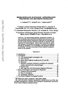
in which we establish a one-to-one correspondence between elements of the basis sets {ψi : i = 0, . . . , ∞} and {φ0,0 , ϕj,k : k = 0, . . . , 2j − 1, j = 0, . . . , ∞}. In the present study we adopt the slightly more complicated multiresolution of Alpert (1993) where multiple scaling functions {φi (y) : i = 0, . . . , m − 1} are used to construct V0 . Specifically, we choose φi (y) as the Legendre polynomial of degree i defined on the interval [0, 1]. An orthonormal basis {ϕi (y) : i = R0, . . . , m − 1} for W0 is also established. More precisely, let Um = {u(y) ∈ L2 ([0, 1]) : [0,1] u(y) y m dy = 0} represent the subspace of functions in L2 ([0, 1]) with m vanishing moments. We then construct ϕi ∈ Uj , j = 0, . . . , i + m − 1, with the orthonormality constraint hϕi , ϕj iL2 [(0,1)] = δij , i, j = 0, . . . , m − 1, where δij is the Kronecker delta. The multiwavelet basis functions ϕj,k are then generated by dilations and translations of {ϕi (y) : i = 0, . . . , m − 1}. The resulting basis is unique (up to the sign) and provides a generalization of Legendre and Haar representations. In particular, Legendre polynomials can be obtained by stopping the expansion at the resolution j = 0, while Haar wavelets are obtained for m = 0. If expanded in the Alpert multiwavelet basis, sparse representations are likely to be observed for piecewise smooth functions. Sharp gradients, bifurcations or discontinuities, for example in hyperbolic problems, motivate the use of such dictionaries as multiwavelet with the ability of capturing these local features for which global polynomials may not be adequate (see, e.g., Le Maıtre et al. 2004). In addition to several numerical advantages, the orthogonality property of Alpert multiwavelets is also desirable allowing first- and second-order statistics of u to be evaluated directly from the expansion coefficients. We refer the interested reader to Alpert (1993) for an in-depth derivation of the Alpert multiwavelet basis. The construction of a multiwavelet basis in L2 ([0, 1]d ) with d ≥ 2 – employed in the numerical example of Section 5 – is also discussed in Alpert (1993). Examples of one-dimensional Alpert multiwavelets with 3 and 4 vanishing moments, respectively, are shown in Figure 1.

3. Compressive Sampling of multiwavelet expansions 3.1. Rudiments of Compressive Sampling Compressive Sampling (CS) is a new direction in signal processing that breaks the traditional limits of the Shannon-Nyquist sampling rate for reconstruction of sparse signals. Consider a vector of measurements u = (u(y (1) ), . . . , u(y (M ) ))T ∈ RM of u ∈ L2 ([0, 1]). Assuming that u admits a multiwavelet expansion of the form (Eq. 2.4) with some finite m and resolution j, u can be represented as u = Ψ α, where the so-called measurement matrix Ψ ∈ RM ×P contains the realization of the multiwavelet basis {ψi (y)} corresponding to u and α ∈ RP is the vector of unknown expansion coefficients. Here, P is the cardinality of the truncated multiwavelet basis. Then u has a sparse multiwavelet representation if kαk0 = #{αi : αi 6= 0} P . For a sufficiently sparse u, CS recovers u exactly using some M P measurements by solving an optimization problem of the form min kαks

α∈RP

subject to u = Ψ α.

(Ps )

The sparsest solution α to (Ps ) corresponds to s = 0, i.e., minimizing the `0 semi-norm

96


kαk0 , which is generally NP-hard to compute. To break this complexity, several heuristics based on greedy pursuit, e.g., Orthogonal Matching Pursuit (OMP), and convex relaxation via `1 -minimization, i.e., s = 1, have been proposed, among other approaches. Moreover, several metrics such as the mutual coherence (Bruckstein et al. 2009), or the restricted isometry property (Candes & Tao 2005) have been introduced to provide guarantees on the uniqueness of the sparsest solution to (Ps ) as well as the ability of the heuristic approaches in recovering the solution. In particular, the mutual coherence of Ψ (e.g., see Bruckstein et al. 2009) is defined as µ(Ψ) = max i6=j

|ψiT ψj | , kψi k2 kψj k2

(3.1)

where ψi ∈ RM is the i-th column of Ψ. Note that µ(Ψ) ∈ [0, 1] in general, and that it is strictly positive for M < P . Depending on the sparsity level kαk0 ,, the mutual coherence provides a sufficient condition on the number M of measurements for a successful recovery of α from Ps , as shown in Bruckstein et al. (2009). 3.2. Sparse multiwavelet approximation using Tree-based OMP In the present study, we extend the greedy Tree-based OMP (TOMP) approach of La & Do (2006) and Duarte et al. (2005) to solve (P0 ) for sparse multiwavelet coefficients α. Due to the local nature of the multiwavelet basis, it may occur, for example, that none of the realizations of the random input y – from which the measurement vector u is generated – belong to the support of the i-th basis function ψi , resulting in ψi = 0. In the interest of brevity, only a short description of the adopted greedy algorithms is provided here; detailed expositions are provided in La & Do (2006) and Duarte et al. (2005). Both the TOMP and OMP algorithms are iterative two-staged procedures. In the first sensing stage, basis functions are selected based on the correlation of their corresponding columns in Ψ with the residual vector. While only the most correlated basis is selected in OMP, few additional candidates with high correlations are considered in TOMP. During the second reconstruction stage, each candidate in turn, with associated ancestors, is temporarily added to the active basis set and the corresponding coefficients are evaluated using a standard least squares. Only the candidate (and ancestors) generating the minimum residual is permanently added to the index set and the process is re-iterated. The TOMP algorithm in La & Do (2006) was originally developed for scalar tree representations. We, however, extend that work to account for vector multiwavelet trees, as needed in this work. Algorithm 1 summarizes the main steps of TOMP.

4. TOMP with Importance Sampling A natural way to obtain the samples u is to generate random realizations of the input y and evaluate the corresponding solution u(y). However, for situations where u exhibits, for instance, sharp gradients or discontinuities, such a sampling strategy may not necessarily lead to accurate approximation because the higher-resolution basis functions needed to capture the local structure of u may not be sampled enough to constitute a well-conditioned measurement matrix Ψ. To achieve a local accumulation of samples, where needed, we here propose an Importance Sampling approach that is discussed next. Importance Sampling strategy. Importance Sampling is a well-known variance reduction methodology in Monte Carlo estimations. Sampling is performed according to a modi-


97

Algorithm 1 Tree-based Orthogonal Matching Pursuit algorithm - TOMP inputs: The number of samples M , basis cardinality P . Matrix Ψ Vector u Maximum allowable iterations kmax Tolerance δ. Coefficients γ, ρ outputs: Solution vector α. initialize: k ← 0. Initialize residual r0 ← u. Initialize index set I0 ← {0}. W ← diag(kψi k2 ) ˜ ← Ψ W. Set to unitary columns Ψ ˜ Define I as the set of all columns of Ψ. while krk k2 > δ and k < kmax and card(Ik ) < ρ M do ˜T rk−1 | where i ∈ I \ Ik−1 cik = |ψ i i,M ax ck = maxi {cik : i ∈ I \ Ik−1 } ax } Sk = {i : cik ≥ γ ci,M k for all i ∈ Sk do Fi ← Anc(i). ˜ k with Ik−1 ∪ Fi . Assemble Ψ T ˜ −1 ˜ T ˜ αi = (Ψk Ψk ) Ψk u ˜ k αi k2 r(i) = ku − Ψ end for ik = arg mini∈Sk r(i) Ik = Ik−1 ∪ Fik . rk = rik . end while return: W−1 αk

fied distribution, which promotes the important regions of the input variables and the quantity of interest whose expectation is sought. An insight into the typical wavelet structure of piecewise smooth functions is given in Duarte et al. (2005). In particular, the wavelet coefficients of piecewise smooth functions tend to form connected subtrees within wavelet trees. Additionally, a large wavelet coefficient (in magnitude) generally indicates the presence of a local singularity or sharp gradient. The above considerations form the basis of our sampling strategy. The idea is to concentrate samples at locations where large multiwavelet coefficients are observed while preconditioning the basis to maintain orthogonality. The proposed importance sampling consists of a number of steps that are applied iteratively: (a) A multiwavelet approximation up to a given m and resolution j is obtained by solving (P0 ).

98


(b) The coefficients αi are sorted in decreasing order, based on |αi |/|supp(ψi )|, where |supp(ψi )| is the size of the support of ψi . (c) A sample is drawn in supp(αi ) according to a uniform distribution only if |αi | > αtol (αtol = 1.0 × 10−3 is used in the present study). Preconditioning the basis. Assuming y is uniformly distributed on [0, 1], i.e., ρ(y) : [0, 1] → 1, the direct application of the above modified sampling leads to measurement matrices Ψ with large mutual coherence µ(Ψ). This is because the multiwavelets are orthogonal with R1 respect to the measure ρ(y), i.e., 0 ψi (y) ψj (y) dy = δij . A correction, therefore, is needed to retain orthogonality for sufficiently large M . Let γ(y) : [0, 1] → R≥0 denote the density function according to which the (independent) modified samples y (k) , k = 1, . . . , M , are p ˆ distributed and let ψi (y) = ψi (y)/ γ(y) be the scaled multiwavelet basis. Then, Z 1 M 1 X ˆ (k) ˆ (k) a.s. ψ (y) ψj (y) pi p ψi (y ) ψj (y ) −−→ γ(y) dy = δij , M γ(y) γ(y) 0 k=1

(4.1)

as a result of the strong law of large numbers. In the CS framework, this translates in sampling according to γ(y) and using a modified ˆ = WΨ and the data u ˆ = Wu with the preconditioner matrix measurementp matrix Ψ W = diag(1/ γ(y (i) )) , i = 1, . . . , M . We now discuss how a piecewise constant measure γ(y) can be defined on partitions of [0, 1] associated with a (truncated) multiwavelet representation. We focus on establishing a one-to-one relationship between a scalar wavelet tree and a partition of [0, 1]. Vector trees (whose vertices are arrays of numbers) are used to store multiwavelet representations whereas scalar trees are usually adopted for wavelets. A partition of [0, 1] is built by first forming a scalar connected subtree T , obtained by pruning all vertices with coefficients αi with |αi | < αtol . The leaves (L in total) of T are identified, and their supports form a set of disjoint intervals {Bi : i = 1, . . . , L} which result in the desired partition of [0, 1]. Using the coefficient-driven sampling discussed above, γ(y) is defined as a piecewise constant distribution. In particular, a set of probability masses pi = 2−j (Mi /M ) for every box Bi is considered in which Mi is the number of samples within the interval Bi (with |Bi | = 2−j ), j is the resolution level of the associated leaf, and M is the total number of available samples. A graphical representation of the adaptive Importance Sampling measure γ(y) is illustrated if Figure 1 for the Kraichnan-Orszag problem with one random initial condition. It can be seen how the measure evolves with increasing samples from a uniform distribution to having a major peak close to y = 1/2, where finer scales are observed in the stochastic response.

5. Numerical test: Kraichnan-Orszag problem The Kraichnan-Orszag (KO) problem is derived from simplified inviscid Navier-Stokes equations (Kraichnan 1963), and is expressed as a coupled system of non-linear ODEs. We here adopt a rotated version of the original KO problem du2 du3 du1 = u1 u3 , = −u2 u3 , = −u21 + u22 , (5.1) dt dt dt with initial conditions specified below. In Wan & Karniadakis (2005), the KO problem is used as a benchmark and analytical solutions are provided in terms of Jacobi’s elliptic functions. √ If the set of initial conditions is chosen such that the bifurcation point (u1 , u2 , u3 ) = ( 2, 0, 1) is consistently crossed,


ψi

3.0 2.0 1.0 0.0 -1.0 -2.0 -3.0 0.0

99

10 9 8 7 0.2

0.4

0.6

0.8

1.0

6

y

γ

(a)

5 4

4.0

3

2.0 ψi

2

0.0

1

-2.0 -4.0 0.0

0.2

0.4

0.6

0.8

0 0.0

1.0

0.2

0.4

0.6

0.8

1.0

y

y

(b)

(c)

1

0.4

10

0.2

10

0.0 0.0

0

-1

10 5.0

10.0

15.0 20.0 Time (s)

25.0

30.0

εrel

σ(u1)

Figure 1: Examples of Alpert Multiwavelets with 3 (a) and 4 (b) vanishing moments, respectively. Adaptivity of the Importance Sampling measure with increasing number of samples (c) for the one-dimensional KO problem.

(a)

u1

1.2 1.0 0.8 0.6 0.4 0.2 0.0 0.0

-2

10

10-3 10-4 10-5 0.2

0.4

0.6 y

(b)

0.8

1.0

0

200

400 600 800 1000 1200 1400 Number of samples

(c)

Figure 2: Results for the 1D KO problem. Evolution in time for the standard deviation of u1 (a). Parametric response for u1 at t = 30s as obtained using 106 Monte Carlo realizations ( ) and approximated with the proposed (CS-MW) approach ( )(b). The convergence of σu1 at t = 30s using the Monte Carlo (MC) method ( ) is , , )(c). compared to various independent runs of the proposed strategy (

100


it is shown that the accuracy of the global polynomial approximations (at the stochastic level) deteriorates rapidly with time. 5.1. Results for 1D KO problem Initial conditions for (Eq. 5.1) are assumed to be uncertain and specified as u1 (t = 0) = 1 ;

u2 (t = 0) = 0.2 y − 0.1 ;

u3 (t = 0) = 0,

(5.2)

where y is uniformly distributed on [0, 1]. The stochastic response is evaluated at t = 20s and t = 30s using a multiwavelet dictionary with m = 3 and a resolution up to j = 7. The OMP solver was used with a relative tolerance = 1.0 × 10−4 . The time history of the standard deviation for variable u1 together with the reconstructed response at t = 30s and convergence graphs are illustrated in Figure 2. The error metric rel = |σCSM W −ˆ σ |/ˆ σ is also evaluated where σCSM W is the estimate for the standard deviation calculated with the CS-based multiwavelet expansion and σ ˆ the corresponding exact value, resulting from several millions of Monte Carlo simulations. 5.2. Results for the 2D KO problem at t = 10s The initial conditions of the Kraichnan-Orszag problem are again assumed to be uncertain but this time are functions of two random variables u1 (t = 0) = 1 ;

u2 (t = 0) = 0.2 y1 − 0.1 ;

u3 (t = 0) = 2 y2 − 1,

(5.3)

where y1 and y2 are independent and uniformly distributed on [0, 1]. A two-dimensional multiwavelet measurement matrix is generated with m = 2 and resolution up to j = 4, resulting in a basis of cardinality P = 9216. Figure 3 shows results in terms of sampling distribution, multiwavelet coefficients, and convergence in statistics for the system’s response. As noted from Figure 3, the expansion coefficients produced by the proposed strategy with about M = 2400 samples are comparable to those obtained using a multiwavelet least-squares approximation (where coefficients are evaluated as αLS = (ΨT Ψ)−1 ΨT u with 9 × 104 samples, demonstrating the efficiency of the CSbased reconstruction.

6. Conclusions A novel framework for non-intrusive uncertainty propagation is proposed which combines the ability of a multiresolution approximation in capturing piecewise smooth stochastic responses via Compressive Sampling. Within this framework, an adaptive Importance Sampling strategy is applied in order to increase the efficiency in approximating responses with sharp gradients or discontinuities, for a given number of samples. Finally, the convergence of the method is demonstrated through its application to the Kraichnan-Orszag problem – a non-linear ODE system – with random initial conditions. The proposed approach is particularly efficient under assumptions of mild dimensionality and sparsity of the response in the selected multiresolution basis. Further research will be devoted to progressively reducing the role played by the above assumptions, by exploring new representations and more general reconstruction paradigms.

Acknowledgments The authors would like to thank Paul Constantine for kindly reviewing the paper, providing helpful suggestions and comments. G.I.’s and D.S.’s work is supported un-


y2

1.0 0.8 0.6 0.4 0.2 0.0 0.0

101

100

10-1 0.2

0.4

0.6

0.8

1.0

εrel

y1

(a)

10-2

100 10-1

-3

10

10-2 αi

10-3 10-4 10-5 0 10

-4

10 1

10

2

10 i

3

10

4

10

2

10

(b)

3

10 Number of samples

4

10

(c)

Figure 3: Results for the 2D KO problem. Distribution of 2410 adaptively sampled locations over the unitary square (a). Higher densities can be observed close to y1 = 1/2, as expected. Expansion coefficients as obtained with CS-MW (•) and using least-squares with 9 × 104 samples (2) (b). Convergence profiles for the Monte Carlo (MC) method ( ) and two independent runs of the proposed (CS-MW) approach ( , ) (c). der Subcontract No. B597952, with Lawrence Livermore National Security under Prime Contract No. DE-AC52-07NA27344 from the Department of Energy National Nuclear Security Administration for the management and operation of the Lawrence Livermore National Laboratory. A.D.’s work is supported by the Department of Energy under Advanced Scientific Computing Research Early Career Award DE- SC0006402.

REFERENCES

Alpert, B. 1993 A class of bases in l2 for the sparse representation of integral operators. Siam J. Math. Anal. 24, 246. Bruckstein, A., Donoho, D. & Elad, M. 2009 From sparse solutions of systems of equations to sparse modeling of signals and images. SIAM Review 51 (1). Candes, E. & Tao, T. 2005 Decoding by linear programming. Information Theory, IEEE Transactions on 51 (12), 4203–4215. Chantrasmi, T., Doostan, A. & Iaccarino, G. 2009 Pad´e–Legendre approximants for uncertainty analysis with discontinuous response surfaces. J. Computational Physics 228 (19), 7159–7180. Doostan, A. & Owhadi, H. 2011 A non-adapted sparse approximation of pdes with stochastic inputs. J. Computational Physics 230 (8), 3015 – 3034. Duarte, M., Wakin, M. & Baraniuk, R. 2005 Fast reconstruction of piecewise smooth signals from incoherent projections. SPARS05 . Ghanem, R. & Spanos, P. 2003 Stochastic finite elements: a spectral approach. Dover Publ.

102


Kraichnan, R. 1963 Direct-interaction approximation for a system of several interacting simple shear waves. Physics of Fluids 6, 1603. La, C. & Do, M. 2006 Tree-based orthogonal matching pursuit algorithm for signal reconstruction. In Image Processing, 2006 IEEE International Conference on, pp. 1277–1280. IEEE. Le Maıtre, O., Najm, H., Ghanem, R. & Knio, O. 2004 Multi-resolution analysis of wiener-type uncertainty propagation schemes. J. Computational Physics 197 (2), 502–531. Ma, X. & Zabaras, N. 2009 An adaptive hierarchical sparse grid collocation algorithm for the solution of stochastic differential equations. Journal of Computational Physics 228 (8), 3084–3113. Wan, X. & Karniadakis, G. 2005 An adaptive multi-element generalized polynomial chaos method for stochastic differential equations. J. Computational Physics 209 (2), 617–642. Witteveen, J. & Iaccarino, G. 2012 Simplex stochastic collocation with random sampling and extrapolation for nonhypercube probability spaces. SIAM J. Sci. Comput. 34, A814. Xiu, D. & Hesthaven, J. 2006 High-order collocation methods for differential equations with random inputs. SIAM J. Sci. Comput. 27 (3), 1118. Xiu, D. & Karniadakis, G. 2002 The wiener–askey polynomial chaos for stochastic differential equations. SIAM J. Sci. Comput. 24 (2), 619–644.