[7] Paul D. O'Grady and Barak A. Pearlmutter: âSoft-LOST: EM on a Mixture of Oriented Lines,â International Con- ference on Independent Component Analysis, ...
2007 IEEE Workshop on Applications of Signal Processing to Audio and Acoustics
October 21-24, 2007, New Paltz, NY
SPARSENESS-BASED 2CH BSS USING THE EM ALGORITHM IN REVERBERANT ENVIRONMENT Yosuke Izumi, Nobutaka Ono, Shigeki Sagayama Graduate School of Information Science and Technology the Univ. of Tokyo 7-3-1, Hongo, Bunkyo-ku, Tokyo 113-8656, Japan {izumi,onono,sagayama}@hil.t.u-tokyo.ac.jp ABSTRACT In this paper, we propose a new approach to sparseness-based BSS based on the EM algorithm, which iteratively estimates the DOA and the time-frequency mask for each source through the EM algorithm under the sparseness assumption. Our method has the following characteristics: 1) it enables the introduction of physical observation models such as the diffuse sound field, because the likelihood is defined in the original signal domain and not in the feature domain, 2) one does not necessarily have to know in advance the power of the background noise since they are also parameters which can be estimated from the observed signal, 3) it takes short computational time, 4) a common objective function is iteratively increased in localization and separation steps, which correspond to the E-step and M-step, respectively. Although our framework is applicable to general N channel BSS, we will concentrate on the formulation of the problem in the particular case where two sensory inputs are available, and we show some numerical simulation results. 1. INTRODUCTION Blind source separation (BSS) has been intensively investigated since this problem setting matches very well the real environment. In the overdetermined case of BSS, the source separation can be performed satisfactorily, especially in clean environment, for example by using Independent Component Analysis (ICA). In order to be able to handle a more realistic situation, however, one must take into account the underdetermined case, where there are less sensors than sources, and reverberation. Many methods for BSS based on speech sparseness where the sources outnumber the microphones have thus been discussed [1, 4, 6, 8, 10] . If the time-frequency components of each source signal are sparsely distributed, then these components rarely overlap with each other even when many sources are mixed together [2]. More specifically, it is assumed that the energy at some time-frequency point originates completely from only a single source. Time-frequency masking aims at extracting the time-frequency components dominated by the target signal. As the time-delay and the amplitude ratio between multiple sensory inputs at each time-frequency point correspond to the direction-of-arrival (DOA) of the signal, the timefrequency mask can be built by performing a clustering on these quantities [1, 5] or by fitting some distribution using the EM algorithm in the feature domain [10]. To make time-frequency masking perform better, one must have a representation which sources become sparser. Araki et al. discussed the time-frequency resolution to reduce musical noise [3]. But most of the separation methods based on time-frequency masking suffer from the fact that clustering in the feature domain becomes difficult in environments where
reverberation and background noises exist, as time-delays and amplitude ratios resulting from each sound source then tend to spread and overlap. Fig. 1 shows time-delays observed by two microphones from three sources with different reverberant times. One can see clearly that reverberation makes clustering difficult. Note that there is another approach to separation which assumes a prior probability distribution on the source signals and estimates simultaneously the parameters of the distribution, the source signals and the mixing process. Most of these methods assume instantaneous mixture and require a very long computation time because they estimate many parameters for example through the EM algorithm with a large number of gaussians, MCMC, or Gibbs sampling [6, 7, 8, 9]. The main difficulty faced by time-frequency masking approaches is the overlap between distributions in the feature domain generated by reverberation. Estimation problems based on Gaussian mixture models deal well with overlapped distributions and estimate distribution parameters with a good accuracy. While usual clustering assigns 0 or 1 to each data whether it corresponds to a member of a cluster or not, Gaussian mixture models assign a continuous value to each data corresponding to the probability to be a member of a cluster. The key idea which makes the estimation of overlapped distributions possible is to obtain the maximum likelihood solution by model fitting. This framework has become very popular as there exists an effective method to obtain this solution, called the EM algorithm. We propose a new method to design a time-frequency mask by applying this key idea to BSS in signal domain instead of feature domain based on speech sparseness. It works well even in a reverberant environment thanks to the properties we described above. This method has the advantage of integrating two processes, clustering-based source localization and masking-based source separation, by maximization of a common objective function while previous methods usually handle the two steps separately. 2. CONCEPT AND MOTIVATION We start by considering the probability p(M (τ, ω)| θ) that the observed signal M (τ, ω) at time-frequency point (τ, ω) arrived from the source direction θ, which we shall call single direction likelihood. We assume throughout this paper that input signals have been transformed into a time-frequency representation, in which speech signal is more likely to be sparse. If the direction likelihood can be determined, we can obtain the maximum likelihood source direction θM L for the case where there is N = 1 source as the direction maximizing the summation of the log-likelihood on all the data:
2007 IEEE Workshop on Applications of Signal Processing to Audio and Acoustics
10000
1000
1000
next section, we formulate the BSS problem as a maximum likelihood estimation with the index of the dominant source signal as the hidden variable, under the assumption that only one source is dominant at each time-frequency point.
power
power
10000
100
10
October 21-24, 2007, New Paltz, NY
100
-0.15 -0.1 -0.05 0 0.05 0.1 0.15 time delay [ms]
(a) TR = 0[ms]
10
3. MAXIMUM LIKELIHOOD ESTIMATION OF SOUND DIRECTIONS AND TIME-FREQUENCY MASK DESIGN -0.15 -0.1 -0.05 0 0.05 0.1 0.15 time delay [ms]
(b) TR = 170[ms]
Figure 1: Extracted time-delay histograms for two different reverberation times TR with three source signals X J= log p(M (τ, ω)| θ). (1) (τ,ω)
In the case where there are N > 1 sources, if the source signals are sparse enough such that only one source signal is dominant at each time-frequency point, we can estimate the nth source direction θn by maximizing the summation of the log-likelihood on the set Ωn of time-frequency points (τ, ω) where the nth source is dominant: X Jn = log p(M (τ, ω)| θn ) (2) (τ,ω)∈Ωn
Note that obtaining Ωn is equivalent to performing source separation by time-frequency masking. In other words, under the assumption that only one source signal is dominant at each timefrequency point, source localization and source separation are mutually related: 1) if Ωn is obtained (source separation), we can obtain θn (source localization), and conversely 2) if θn is obtained, we can obtain Ωn . Some previous works based on masking performed source separation in two steps. The feature quantities such as the time-delay were first extracted and clustered for example using voting methods, k-means clustering or distribution fitting in the feature domain. Then a time-frequency mask was built and the signals separated. The problem we face is basically a clustering problem to divide the time-frequency domain into parts corresponding to each source signal. The estimation of Gaussian mixture models (GMM) is often a good solution in such contexts. While some methods already apply GMM to overlapped distribution in the feature domain, we need to apply it in the original signal domain because the observation error follows the Gaussian distribution in signal domain, not in the feature domain. The problem is here to estimate each Gaussian’s mean and variance when each data point is assumed to have been generated by one of the Gaussians but one does not know which Gaussian generated it. If we now consider 1) the observed signal M (τ, ω) at time-frequency point (τ, ω) as a data point, 2) direction likelihood distributions corresponding to each source as Gaussian distributions, 3) parameters of the direction likelihood distributions as the means and variances of Gaussian distributions, one can see that the GMM problem is equivalent to the 2ch BSS problem. Using GMM thus enables to estimate parameters robustly even in the case where distributions overlap each other, which often occurs in reverberent environments as shown in Fig. 1. Introducing this method for BSS based on speech sparseness, source localization/separation will perform well even when observed feature quantity distributions overlap because of reverberation or background noise. A common effective approach for maximum likelihood estimation in mixture models like GMM is the EM algorithm. In the
3.1. Observation model with diffused noise covariance Let M (τ, ω) = (ML (τ, ω), MR (τ, ω))T be observed signals by two microphones represented in time-frequency domain. Assuming that 1) source signals are sparse enough such that only one source signal is active at each time-frequency point, and 2) each source signal is transfered as a plane wave, M (τ, ω) can be written as M (τ, ω) = Sk (τ, ω)bk + N (τ, ω), (3) where Sk (τ, ω) is the source signal which is active in (τ, ω), k(τ, ω) is the index of the source, bk = (1, exp(jωδk ))T is the transfer function from the source to microphones (δk is a time delay between two microphones), and N (τ, ω) = (NL (τ, ω), NR (τ, ω))T is the observation error which includes reverberation and background noise and is assumed to be independent from the source signals. For simplicity, we will abbreviate (τ, ω) and only write Sk , M , N when there is no ambiguity. If ideally N (τ, ω) is zero, the vector M is always parallel to bk and the time delay between ML and MR is identical to δk . The deviation of the time delay in real situation is caused due to N (τ, ω). The advantage of the observation model in signal domain is to naturally introduce the physical behavior of N (τ, ω). A representative example is the diffused sound field model [11, 12], which models the reverberation as waves coming from all directions stochastically. According to this model, the noise correlation matrix V = E[N N H ] is of the form „ « 1 sinc(ωD/c) V = σ2 (4) sinc(ωD/c) 1 where D represents the distance between the two microphones and c is sound velocity. Under the assumption that N follows a Gaussian distribution with mean 0 and covariance matrix V , the loglikelihood is given by 1 log p(M | δk ) = − log(2π) − log |V | 2 1 − (M − Sk bk )h V −1 (M − Sk bk ). (5) 2 The equation includes the unknown parameter Sk . One can think of several ways to estimate Sk . One way we develop here, is to use Sk which gives maximum likelihood: ∂ log p(M | δk ) =0 ∂Sk∗
⇔
Sk =
bhk V −1 M . bhk V −1 bk
(6)
Note that the expectation of S is identical to SM L under the Gaussian distribution of N , which is used in a mask design for separation, later. Substituting eq. (6) into eq. (5), we obtain the likelihood of M for the direction corresponding to a time delay δk as log p(M | δk ) = − log 2π|V |−M h V −1 M +
|bhk V −1 M |2 . bhk V −1 bk
(7)
Our goal is to obtain the source direction set and the noise power θ = (δ1 , · · · , δK , σ 2 )k that maximizes
2007 IEEE Workshop on Applications of Signal Processing to Audio and Acoustics
X
J=
log p(M (τ, ω)| θ),
(8)
(τ,ω)
October 21-24, 2007, New Paltz, NY
3.3. Explicit form of Q function Using eqs. (4), (7), and (13), the explicit form of Q function in eq. (12) corresponding to the kth source is derived as below:
where p(M (τ, ω)| θ) represents the likelihood of observation M (τ, ω) (t) when the source signal is in the direction (δ1 , · · · , δK ) and the Q(δk ; δk ) (14) 2 noise power σ . In this paper, we assume that the number of „ « (t) X mτ,ω,k |bh V −1 M |2 source K is known and noise variance was the same at every time= − log 2π|V | − M h V −1 M + kh −1 2 2 frequency component. Note that it is easy to extend σ to a varibk V bk (τ,ω) ance σω2 depending on frequency. ˛ „ « „ «˛2 q q ˛ 1 X ˛˛ (t) (t) ˜ L − e−jωδk ˜R ˛ , = C0 + m M m M τ,ω,k τ,ω,k ˛ ˛ C1 (τ,ω) 3.2. Applying the EM algorithm to localization of multiple sparse sources where C0 , C1 are constant terms. In eq. (14), the noise-uncorrelated On the assumption that only one source is dominant at each time˜ = (M ˜ L, M ˜ R )T = V − 12 M is multiplied by the observation M q frequency point, this can be marginalized to (t) square root of the partition function mτ,ω,k , which plays a soft X time-frequency masking. p(M (τ, ω)| θ) = p(M (τ, ω)| k(τ, ω), θ) k
=
X
p(M (τ, ω), k(τ, ω)| θ)p(k(τ, ω)), (9)
k
where k(τ, ω) represents the index of the dominant source at (τ, ω), or the missing data as we cannot actually observe it. Transposed to the GMM case, it corresponds to the index of the Gaussian which generates the observed data. If k(τ, ω) is given, the likelihood in eq. (8) depends only on the kth source direction, and can be simplified to 2
p(M (τ, ω), k(τ, ω)| θ) = p(M (τ, ω)| δk , σ ).
(10)
For maximum likelihood estimation including missing data, the EM algorithm introduces an auxiliary function called the Q function defined using a tentative parameter (here a tentative source direction) θ (t) . The parameters are then estimated by sequential iteration of two steps: • E step: calculate Q(θ; θ (t) ).
• M step: update θ (t) by θ (t+1) = argmaxθ Q(θ; θ (t) ). The Q function in our problem is Q(θ; θ (t) ) =
X
(t)
Q(δk ; δk ),
(11)
k
3.4. Update equations of the parameters Our proposed method can also estimate the noise variance from the observation by differentiating the Q function with respect to σ 2 . So, update rules are summarized as follows: (t)
p(M (τ, ω)| δk , (σ 2 )(t) ) (t) mτ,ω,k = P , (t) 2 (t) ) k0 p(M (τ, ω)| δk0 , (σ ) (t+1)
δk
(t)
= argmax Q(δk ; δk ).
(15) (16)
δk
` 2 ´(t+1) σ =
(t)
mτ,ω,k 1 X 2 2C 1 − sinc (ωD/c) τ,ω,k „ « bh V −1 M × M h V −1 M − kh −1 , bk V bk
(17)
(t)
where V and bk in eq. (17) includes (σ 2 )(t) and δk , respectively, and C represents the total number of time-frequency points. Since eq. (16) cannot be analytically solved, the update is done by cal(t) culating Q(δk ; δk ) for all the discretized δk and selecting the maximum. 3.5. Mask design for separation After the estimation of (δ1 , · · · , δK ) and σ 2 by the EM algorithm, the expectation of the kth source signal can be calculated as X E[Sk ] = p(k)Ek [Sk ] + p(k0 )Ek0 [Sk ] k0 6=k
where (t)
Q(δk ; δk ) =
X
= (t)
mτ,ω,k log p(M (τ, ω)| δk , (σ 2 )(t) ),(12)
(τ,ω) (t)
mτ,ω,k =
(t) p(M (τ, ω)| δk , (σ 2 )(t) ) . P (t) 2 (t) ) k0 p(M (τ, ω)| δk0 , (σ )
(13)
The multiple source localization problem is broken down into several single source localization problems, as the Q function is broken down into the summation of functions which only depend on (t) each θk , as shown in eq. (11). The quantity mτ,ω,k calculated at the E step is called partition function and stochastically distributes the contribution from each time-frequency component M (τ, ω) to the likelihood. This gives us a framework to deal with ambiguous data for which clustering was difficult.
bhk V −1 (mτ,ω,k M ) , bhk V −1 bk
(18)
where p(k) is the probability that kth source is active, and Ek0 [Sk ] is the expectation of Sk when k0 th source is active. Since only one source signal is active at each time-frequency point, Ek0 [Sk ] = 0 for k0 6= k. So, the partition function mτ,ω,k itself, instead of its square root in the localization step, works a soft mask in the separation step. 4. EXPERIMENTAL EVALUATION We evaluated the separation performance in anechoic and reverberant environments through simulations. For the tests in reverberant environment, the speech data and its reverberation were calculated and mixed by mirror method in
2007 IEEE Workshop on Applications of Signal Processing to Audio and Acoustics
5. CONCLUSION
S3
ML
60
4cm M R
45
October 21-24, 2007, New Paltz, NY
S2
S1
Figure 2: Setup of sources and microphones Table 1: Source localization results (time-delay [µs]) Condition Method s1 s2 s3 TR = 0 [ms] DUET -12.7 0.0 7.7 TR = 0 [ms] proposed -9.8 0.0 6.7 TR = 370 [ms] DUET 0.2 1.0 19.2 TR = 370 [ms] proposed -12.3 0.0 10.3 actual value -12.7 0.0 10.4 Table 2: Source separation results (SNR [dB]) Condition Method s1 s2 s3 TR = 0 [ms] DUET 15.0 12.5 7.9 TR = 0 [ms] Mandel 12.5 8.7 8.6 TR = 0 [ms] proposed 18.3 14.1 12.3 TR = 370 [ms] DUET 3.7 -7.8 0.9 TR = 370 [ms] Mandel 5.6 1.2 4.8 TR = 370 [ms] proposed 10.0 3.2 7.7 Table 3: Relation between TR and estimated σ 2 TR [ms] 0 90 170 270 370 σ2 0.12 0.14 0.17 0.21 0.25
a simulated room illustrated in Fig. 2 whose reverberation time was TR = 370ms. For the original speech, we used Japanese sentences spoken by male and female speakers. The STFT frame size was 1024 and the frame shift was 512 at a sampling rate of 16kHz based on the discussion by Yilmaz et al. [1]. We stopped the iterations of the EM algorithm when the increment of the Q function became less than a threshold. As a comparison, we used the “DUET” by Yilmaz et al. [1] and the soft masking method using EM algorithm by Mandel et al. [10], which we will refer to as the previous method in the following. Source localization results of only DUET and proposed method are shown in Table 1 because the method by Mandel et al. does not identify a certein location of sources. We used the gain of SNR as a measure of separation performance. Table 2 shows source separation results. Both the previous and proposed methods can estimate source location accurately in anechoic environment, but in a reverberant environment, the previous method cannot perform neither clustering nor separation, while the proposed method shows good performance for source localization and separation. Table 3 shows the relation between reverberation time and σ 2 estimated by the proposed method. Note that σ 2 has the same unit as the power of the observation signal but it is not notified here. We can see that the noise variance estimated by our method varies according to the environment. The proposed method takes at most 10s to separate three sources from two mixtures with length 5s on a 2.8GHz CPU machine.
We proposed a method for underdetermined source separation by applying the EM algorithm to a sparseness-based approach. In parallel with the general EM algorithm, the hidden variable corresponds to the index of the source signal, the E-step to source separation and the M-step to source localization respectively. The objective function of our method is common for the separation and localization steps, while previous methods performed source localization and separation as separate steps. Through a simulation experiment, we confirmed that our method can efficiently separate the observations even in a reverberant environment. We plan to evaluate our method in real environment and to introduce a noise model appropriate for reverberation and a microphone model taking into account sensitivity differences. In addition, our framework enables model selection using information criteria, leading to the estimation of the number of sources, since the problem is formulated as a maximum likelihood one. 6. REFERENCES [1] O. Yilmaz and S. Rickard: “Blind Separation of Speech Mixtures via Time-Frequency Masking,” IEEE Transaction on Signal Processing, Vol. 52, No. 7, pp 1830-1847, 2004. [2] S. Rickard and O. Yilmaz: “On the Approximate W-disjoint Orthogonality of Speech,” Proc. ICASSP, Vol. I, pp. 529-532, 2002. [3] S. Araki, S. Makino, H. Sawada, and R. Mukai: “Reducing Musical Noise by a Fine-Shift Overlap-add Method Applied to Source Separation using a Time-Frequency Mask,” Proc. ICASSP, vol. III, pp. 81-84, 2005. [4] L. Vielva, D. Erdogmus, C. Pantaleon, I. Santamaria, J. C. Principe: “Underdetermined Blind Source Separation in a Time-Varying environment,” Proc. ICASSP Vol. III, pp30493052, 2002. [5] S. Winter, H. Sawada, S. Araki and S. Makino: “Overcomplete BSS for Convolutive Mixtures Based on Hierarchical Clustering,” Proc. SAPA2004, S1.3, 2004. [6] S. Winter, H. Sawada, S. Makino: “On Real and Complex Valued L1-norm Minimization for Overcomplete Blind Source Separation,” Proc. WASPAA2005, pp. 86-89, 2005. [7] Paul D. O’Grady and Barak A. Pearlmutter: “Soft-LOST: EM on a Mixture of Oriented Lines,” International Conference on Independent Component Analysis, pp. 428-435, 2004 [8] C. Fevotte and S. J. Godsill, “A Bayesian Approach for Blind Separation of Sparse Sources,” IEEE Trans. on Speech and Audio Processing, Vol. 14, No. 6, pp 2174-2188, 2006. [9] A. T. Cemgil, C. Fevotte, and S. J. Godsill. “Blind Separation of Sparse Sources using Variational EM,” Proc. 13th EUSIPCO, 2005. [10] M. Mandel, D. Ellis and T. Jebara, “An EM algorithm for localizing multiple sound sources in reverberant environments,” Proc. Neural Info. Proc. Sys., 2006. [11] R. K. Cook, R. V. Waterhouse, R. D. Berendt, S. Edelmann and M. C. Thompson, “Measurement of correlation coefficients in reverberant sound fields,” JASA, Vol. 27, No. 6, pp. 1072-1077, 1955. [12] I. A. McCowan, H. Bourlard, “Microphone Array Post-Filter Based on Noise Field Coherence,” IEEE Trans. on Speech and Audio Processing, Vol. 11, No. 6, pp. 709-716, 2003.