Spatial and Polarisation Correlation Characteristics for UWB Impulse Radio Junsheng Liu, Ben Allen
Wasim Q. Malik, David J. Edwards
Center of Telecommunication Research King’s College London, Strandg WC2R 2LS London, UK Email: junsheng.liu,
[email protected]
Department of Engineering Science University of Oxford Parks Road, OX1 3PJ Oxford, UK Email:wasim.malik,
[email protected]
Abstract— Correlation between diversity branches is the key parameter in determining the diversity performance of wireless systems. In this paper, measurements in a temporally and spatially stationary indoor environment are carried out to obtain the channel impulse responses for the UWB impulse radio using receivers with different positions or different polarisation states. A two-dimension (2D) RAKE receiver with post-detection equal gain combining (EGC) diversity is assumed to be used. Three definitions of correlation coefficients of the diversity branches are considered: correlation coefficient, normalized correlation and channel profile correlation, will be analysed in this paper. The results show that the normalised correlation is more effective to assertain the degree of similarity of the correlated diversity branches where medium scale fading dominates.
I. I NTRODUCTION UWB has been one of the hot topics in wireless industry and academia since the early 1990s, and has become a candidate for high data rate transmissions over short ranges. UWB impulse radio occupies a frequency bandwidth from 3.1GHz to 10.6 GHz, assigned by the Federal Communications Commission (FCC) [1] in 2002, and thus results in an extremely short pulse width, in the order of a nanosecond (ns). One of the advantages of UWB impulse radio lies in fully resolving the multi-path. Different configurations of RAKE receiver have been proposed in [2] and [3] in order to exploit the inherent multi-path delay diversity of the UWB channel. UWB wireless have been proposed with data rates from hundreds of Mbps to several Gbps over a range of 1 to 10m and even tens of meters [4], with a trade-off between range and data rate. Diversity combining has been developed over several decades as a means of increasing the wireless communication capacity. The four basic diversity combining schemes are: maximum ratio combining (MRC); equal gain combining (EGC); selection combining(SC) and switched diversity. Many papers and books have exploited or summarised the basic principles for these combining schemes, see [5], [6] and [7] for example. There are several dimensions that can be exploited in diversity systems. Two of them are space and polarisation. In the case of spatial diversity, the closer the receivers are located together, higher signal correlation and lower level of mean power difference are experienced by the receivers due to similar scattering environments experienced by the antennas. Polarisation diversity exploits diversity between the vertical and horizontal polarised waves.
The UWB spatial diversity system considered in this paper can be considered as a 1 × 2 SIMO configuration with one transmit antenna and two receive antennas. This is receive diversity, but due to channel reciprocity can also be considered as transmit diversity. Whilst the UWB polarisation diversity system considered here can be regarded as a 2 × 2 MIMO configuration with two orthogonal polarised transmit antennas and two orthogonal polarised receive antennas. Many works have found the expressions of the probability density function (PDF) of the combined outputs of the diversity branches for narrow band systems exploiting different combining schemes over different kinds of fading channels and is summarised in [11]. However, finding the exact PDF for the combined received UWB impulse signals in a diversity system is not the goal of this paper. Instead, this paper reports the behavior of the correlation of the UWB impulse signal which acts as a key parameter in the expression for the PDF of the combined outputs and pave the way for further system performance analysis. In order to present the background of the analysis, a brief introduction to the distribution of the outputs of the RAKE receiver for the UWB impulse radio is also included later in this paper. The remainder of this paper is organised as follows: the channel model used for the UWB impulse radio is introduced in section II; the combined outputs of the RAKE receivers are given in section III; a 2D diversity RAKE receiver and the definition of the three kinds of correlations are given in section IV; the measurement methodology is given in section V; the analysis for the correlations based ont the measurement results are presented in section VI; conclusion is given in section VII. II. C HANNEL MODEL FOR THE UWB IMPULSE RADIO Based on the modified version of the S-V channel model [8], the IEEE 802.15.3a standard task group has established a standard channel model [9] for the indoor UWB propagation. For the sake of easy data processing, a tap delay line channel model, instead of the standard channel model, is used in this paper. The tap delay line channel model is constructed based on the resolvable time delay bins of the UWB impulse radio as follows: N −1 X ai δ(t − i · ∆τ ) (1) h(t) = i=0
where ∆τ is the minimum resolved time bins, which is approximately the reciprocal of the bandwidth occupied by the transmitted signal; N is the total number of the resolved time bins, which can be calculated as N = Texcess /Tp , where Texcess is the channel excess delay and Tp is the pulse width. For the first arriving component the delay is zero. ai is set to be zero when there is no multi-path component appearing in the ith time bin. In the data processing procedure, the realized channel in equation (1) can be treated as a channel vector: H = [a1 a2 ...aN ]
(2)
where ai is the magnitude for each time delay bin in equation (1). III. O UTPUT SIGNAL AT THE RAKE RECEIVER A post-detection RAKE receiver [11] is utilised in each diversity branch in this paper for its simple realisation, which only requires the channel information of time of arrival and magnitude of the multi-path fingers. Assume the transmitted signal is s(t). The received signal on the k th receiver, rk (t) is given as:
=
ai,k · s(t − i · ∆τ ) + n(t)
th
where hk (t) is the channel impulse response for the k receiver, ⊗ denotes convolution, and n(t) is the additive white Gaussian noise. The impulse response of the match filter on the receiver side is h∗ (−t) ⊗ s∗ (−t), which matches both the transmitted signal and the multi-path channel. ∗ stands for the conjugate operation. The received signal energy, dk , after detection for the k th receiver at t = 0, can be given as: dk = rk (t) ⊗ h∗ (−t) ⊗ s∗ (−t)|t=0 N −1 X
ai,k aj,k · p(τi,k − τj,k ) + nk
=
i=0 N −1 X
|ai,k |2 · p(0) + nk (6) 2
|ai,k | + nk
i=0
where p(0), the transmitted signal energy, and can be normalized to 1. |ai,k |2 is namely the signal power of the ith finger in the k th receiver, but is regarded as signal energy in this paper because of the effect of the normalisation. In the rest of the paper, the noise component is not included in the correlation analysis for the outputs of the RAKE receiver. For the selective RAKE (S-RAKE) receiver [10], the detection output can be given as: X |ai,k |2 (7) dk = i∈S
where S is the aggregate of the S multi-path components with highest magnitude. And for the partial RAKE (P-RAKE) receiver [10], the detection output can be given as: X |ai,k |2 (8) dk =
(4)
IV.
CORRELATED OUTPUTS OF THE
A. a 2D diversity RAKE receiver structure A 2D diversity system consisting L antennas, each of which is followed by an N-finger RAKE receiver, is utilised in this paper. For a diversity system of two antennas followed by RAKE receivers, the combined signal energy is given below and is similar to equation (6): D=
where nk is the noise component at the output of the RAKE receiver, and p(τ ) can be given as:
(5)
−∞
For τ ≥ Tp , p(τ ) = 0. Assume that for high enough bandwidth, ∆B, all the multipaths can be resolved and the arriving pulses do not overlap, which means |τi,k − τj,k | ≥ Tp for any i 6= j. This is true for the propagation environment where the difference between c any two of the multi-path lengths is larger than ∆L = ∆B = 4cm, where c is the speed of the light in the air. Under this
−1 L N X X
k=1 i=0
where dk =
∗
RAKE RECEIVERS
In this section, an introduction is first given to the 2D diversity RAKE receiver which employs post-detection EGC. Then a brief description on the statistics distribution of the RAKE receiver combining result are introduced before giving the definition and meaning of the normalized correlation, the correlation coefficient of the received signals and the correlation of the channel profiles.
i,j=0
p(τ ) = s(t − τ ) ⊗ s (−t)|t=0 Z ∞ = s(α)s∗ (α − τ )dα
N −1 X
where P is the aggregate of the first P multi-path components. (3)
i=0
=
dk =
i∈P
rk (t) = s(t) ⊗ hk (t) + n(t) N −1 X
assumption, equation (4) can be further simplified as:
N −1 X
|ai,k |2 =
N −1 X i=0
di =
L X
dk
(9)
k=1
|ai,k |2 , k = 1, 2...L is the combined outputs
i=0
of the N RAKE fingers following the k th receiver, and L X |ai,k |2 , i = 0, 2...N − 1 is the combined results di = k=1
over all the receivers for the ith RAKE finger. Because correlation between multi-path components is negligible [12], L X |ai,k |2 can be assumed to be independent of each di = k=1
other and the correlation between the receive antennas is included in each di and is thus difficult to analyse. On the
other hand, the correlation of the outputs of different diversity branches lies between the combined results of each RAKE N −1 X |ai,k |2 . For the EGC combining, dk are receiver, dk = i=0
simply summed, and the correlation between dk is of interest and will be analysed in the rest of this paper. B. the statistical distribution of the RAKE receiver combining result Due to the short pulse width in the time domain for the UWB impulse system, the multi-path components are less likely to overlap at the receiver compared to a narrow-band communication system. Thus the central limit theorem may not be applied to result in Rayleigh fading or Rician fading on the receiver side. A more general statistical distribution, the Nakagami-m distribution, can be applied for the received pulse magnitude in the fading environment. The PDF of the received pulse magnitude, a, in the Nakagami-m fading environment can be given as below [11]: ¶ µ ma2 2mm a( 2m − 1) (10) exp − pa (a) = Ωm Γ(m) Ω where a ≥ 0 and Ω = E{a2 }. E{·} is the expectation operation. The amount of fading (AF1 ) of the Nakagami-m fading environment is given as AF = 1/m; γ = a2 , where a is Nakagami-m distributed, obeys the gamma distribution with the PDF shown as followed: ¶ µ mγ mm γ ( m − 1) (11) exp − pγ (γ) = γ m Γ(m) γ where γ ≥ 0. Since the gamma distribution is, in essence, a chi-square distribution, and the sum of chi-square distributed variables is still chi-square distributed, the distribution of dk can be given by equation (11). C. correlation coefficient of the received signals Correlation coefficient enables the degree of similarity of two received signals originating from the same source and propagating through different but correlated wireless channels to be assertained. The correlation coefficient of the outputs, d1 and d1 , of the RAKE receivers following the two receiver antennas with different locations or polarisations is given as [6] [7]: cov(d1 (t), d2 (t)) σ1 σ2 E{(d1 (t) − m1 )(d2 (t) − m2 )} = σ1 σ2
ρcc =
(12)
where mi = E{di (t)}, i.e. the mean of di (t), and σi = q 2 E{(di (t) − mi ) }, i.e. the standard variance of di (t). The subscript i is the index of the receiver antenna. ρcc ranges between [−1, 1]. 1 The
definition of AF is given as: AF = on AF, please refer to [11]
var(prake ) . (E{prake })2
For more details
The ’minus’ operation in the numerator of equation (12) leads to a similarity comparison of the fluctuation of the signals around their mean values for different antenna branches. For branches in a diversity system with relatively small signal energy fluctuations comparing to the their mean values, that is, the fading is not severe compared to the mean signal value, the magnitudes of the signals from different diversity branches may look very similar to each other. However, there may be a low correlation coefficient between them. Their unsimilarity can not be sensed unless the the signals are investigated in small scale. This scenario is true for the fading environment where medium scale fading, such as fading caused by shadowing which can be described by a Log-Normal distribution and approximated by Gamma distribution [11], dominates. For different branch receivers located in the same shadowing or non-shadowing area with little movement and thus AF is relatively small, the correlation coefficient would not make too much sense. D. normalised correlation of the RAKE receiver outputs In contrast to cov(d1 (t), d2 (t)) in equation (12), the correlation of the two real signal d1 (t) and d2 (t), i.e. E{d1 (t)·d2 (t)}, directly compares the magnitude of the two signals. The normalised correlation is given as: ρnc = p
E{d1 (t) · d2 (t)} p E{|d1 (t)|2 } · E{|d2 (t)|2 }
(13)
where 0 ≤ |ρnc | ≤ 1. The normalised correlation of the outputs of the receivers shows the correlation of the diversity branches in the medium scale fading environment instead of the small scale fading environment. For diversity branch receivers staying in the same shadowing area where the multipath fading is small compared to the medium scale fading, the value of ρnc remains high. E. correlation of the channel profiles It is also interesting to compare the propagation environment directly for receivers with different locations or different polarisation states. The correlation coefficient of the channel vectors, Hi , expresses the degree of similarity for different channel profiles. The spatial correlation coefficient for the channel profiles is given as: ρch (d) = p
E{H∗k · Hl } p E{H∗k · Hk } E{H∗l · Hl }
(14)
where H∗ stands for the matrix operation of conjugate transpose for the vector H. The channel vector Hk and Hl represent the channel profiles for receiver k and l with a distance of d. V. M EASUREMENT M ETHODOLOGY In order to investigate the spatial and polarisation correlation behavior for a UWB impulse radio, channel measurements have been carried out. The measurement took place in a typical indoor office environment, as shown in figure 1. In order to maintain spatial and temporal stationarity, no body enters the room and no object in the room moves during the measurements. The measurement process was completely automated,
and calibration was completed before the measurement was started. The receive antenna was mounted on top of an xy-positioner whilst the transmit antenna was fixed. The positioner moved the receive antenna in a 1 m x 1 m square grid with a 0.01m spacing. At each point in this grid, the complex frequency transfer function was measured using a vector network analyser (VNA). The frequency span, fsweep , covered the FCC UWB band, i.e., 3.1 GHz to 10.6 GHz. In this band, channel sounding was performed at nf = 1601 individual frequencies, yielding a frequency resolution of fres = fsweep /nf = 4.6875 MHz, which corresponds to a maximum delay profile length of 1/fres = 213.3ns. The channel impulse response for each receiver position can be achieved by the inverse fast fourier transform (IFFT) operation on the data in the frequency domain. The resolution of the impulse response can be calculated as ∆τ = 1/fsweep = 0.133ns. The distance between the transmit antenna and the center of the measurement grid is 4.5m. Both the Tx and the Rx were 1.5 m above the floor. For the Line-of-Sight data set, a clear line of sight was present, whilst for the non-Line-of-sight (nLoS) case, a large grounded aluminium sheet was placed between the transmit and receive antennas in order to block the direct path. Only one Tx and one Rx location are measured at a time. The Tx and Rx may be vertically or horizontally polarised. In order to get the channel profile for the 1 × 2 SIMO and 2 × 2 MIMO diversity system, two and four measurement campaigns need to be carried out, respectively. It is assumed that the propagation environment remains unchanged during the measurements. VI.
MEASUREMENT RESULTS
The distribution analysis for the RAKE receiver outputs are first given in this section before the analysis results for the correlation coefficients, normalised correlation and channel profile correlation. A. PDF of the RAKE receiver outputs The curve of the PDF based on the measurement data and the theoretical PDF of equation (11) for the outputs of the S-RAKE receiver in the LoS scenario making use of all the fingers, the strongest 50 fingers and strongest 10 fingers are presented in figure 2. It can be seen that the outputs of the RAKE receiver obey the gamma distribution very well with different values of the parameter m. Because larger m corresponds to less fading, it can be seen that S-RAKE with more fingers suffers less fading than those with less fingers. B. correlation coefficient The spatial correlation coefficient for the S-RAKE receiver in the LoS and nLoS scenarios, employing a vertical polarised Tx to a vertical polarised Rx, are shown in figure 3, figure 4, respectively. It can be seen that the correlation coefficient decays very fast as the inter-sensor distance increases. However, considering the the amount of fading shown in table I, it is obvious that this correlation coefficient just shows the
similarity of the fluctuations of the RAKE combining results of different receivers with a certain distance. The correlation coefficient between the branches of the vertical polarised Tx to the vertical polarised Rx and the horizontal polarised Tx to the horizontal polarsed Rx are tabulated in table II. Because both the magnitudes of the received signals from the vertically polarised and horizontally polarised antennas are large comparing to their fluctuations around the mean values, the correlation coefficient of different diversity branches with different polarisation states remains very low as well. C. normalised correlation of the outputs of the RAKE receiver The normalised spatial correlation of the output of the RAKE receivers for the different kinds of RAKE receivers, for both LoS and nLoS scenarios are presented in figures 5, 6, 7 and 8. It can be seen that for most the time, the normalised correlation remains obove 0.8, which implies that the outputs of the RAKE receivers in the diversity system stay of the same level with a high probability. This is because in the measurement methodology presented in this paper, the whole, or most the area within which the receivers move around, is in the same shadow or non-shadow area. The inter-sensor distance needed to reduce the probability of the diversity branches suffering medium-fading area at the same time is out of the measurement range presented in this paper. Thus, based on the measurement results shown in this paper, spatial diversity may not be practical in the personal area network because of the requirement for the large inter-sensor distance (> 1m in this measurement). However spatial diversity may still find its stage in the UWB impulse radio sensor network where larger element spacings may be more practical. This could utilise the virtual antenna array principal described in reference [14]. Further measurements are needed to find out the inter-sensor correlation distance [13] to achieve low normalised correlation in environment where the medium scale fading dominates if both the two orthogonally polarised antennas are located close to each other and suffer from the same medium scale fading. For polarisation diversity, the normalised correlations are listed in table II. It can be seen that the polarisation diversity branches also suffer high normalised correlation as the spatial diversity branches do, hence the usage of polarisation diversity in UWB impulse radio systems will not yield large performance gains. D. Spatial correlation of the channel profiles The spatial correlation coefficient of the channel vectors for LoS and nLoS scenarios, vertical Tx to vertical Rx and horizontal Tx to horizontal Rx are given in figure 9 It can be seen that the correlation coefficient levels off at around 0.6 with d increasing from 10cm to 80cm. This implies that when the channel information of a previous receiver position as far away as 80cm is used in the match filter in the RAKE receiver, the reduction of the received energy is, on average, no more than 3dB. This is because the receiver with different locations share similar propagation characteristics. The difference between the channel vectors implies
small change of the propagation environment caused by the movement of the receiver rather than the random fast fading caused by the overlapping of the multi-path components. VII. C ONCLUSION In a UWB impulse radio employing a 2D diversity system with post-detection EGC, the outputs of the RAKE receivers are correlated Gamma distributed. The graphs of the Gamma distribution PDF can be constructed based on the measurement data. Both the correlation coefficients and the normalised correlation for S-RAKE and P-RAKE configurations in LoS and nLoS scenarios are analysed based on the measurement data. It can be seen that for UWB impulse radio, both the polarisation diversity and the spatial diversity suffer similar medium scale fading, which is mainly caused by shadowing in a measurement area as large as a square meter in a typical office environment. Thus the correlation coefficient of the two Gamma distributed signal may not make too much sense in the diversity combining schemes, while the normalised correlation of the signals can serve as a benchmark for whether the antennas are located in the same shadowing area. The spatial correlation of the channel profiles can be used to determine how often the channel information needs to be updated when the receiver is moving around while receiving UWB impulse radio signals in an indoor environment. More measurements over larger area are needed to observe the correlation behavior for the UWB impulse signal in the office area where the medium scale fading dominates for the impulse radio signals. On the other hand, analysis on the ”amount of fading” versus bandwidth and versus centre frequency is another subject of the future work. VIII. ACKNOWLEDGEMENT The authors wish to thank EPSRC for supporting this research under grant number GR/T21776/01. R EFERENCES
TABLE I A MOUNT OF FADING , V 2 V
type of RAKE receiver
LoS
nLoS
strongest 1 finger strongest 5 fingers strongest 10 fingers strongest 30 fingers strongest 50 fingers first 1 fingers first 5 fingers first 10 fingers first 30 fingers first 100 fingers all fingers
0.2399 01073 0.07 0.0427 0.0362 1.4082 0.09 0.0558 0.0384 0.038 0.0261
0.2568 0.1278 0.0893 0.0597 0.0522 0.6487 0.193 0.1746 0.2724 0.0636 0.0615
TABLE II P OLARISATION CORRELATION COEFFICIENT (CC) AND NORMALISED CORRELATION (NC)
type of RAKE receiver
CC(LoS/nLoS)
NC(LoS/nLoS)
strongest 1 finger strongest 5 fingers strongest 10 fingers strongest 30 fingers strongest 50 fingers first 1 fingers first 5 fingers first 10 fingers first 30 fingers first 100 fingers all fingers
0.01267/0.01162 0.09964/0.10651 0.18054/0.19802 0.30077/0.34322 0.33961/0.39296 0.09484/0.00087 0.25245/0.04395 0.22939/0.01441 0.16934/0.22835 0.19665/0.21030 0.42034/0.3370
0.78532/0.78532 0.89213/0.89213 0.92917/0.92917 0.96122/0.96122 0.96906/0.96906 0.45269/0.7825 0.86692/0.8903 0.89017/0.9260 0.88386/0.9582 0.92694/0.9727 0.98116/0.9577
Glass Window Wooden Bench
Office 364 sq. ft.
6m
[1] Revision of Part 15 of the Commission’s Rules Regarding UltraWideband Transmission Systems, Feceral Communications Commission, First Report and Order, ET Docket, Feb.2002 [2] John D. Choi and Wayne E. Stark, “Performance of Ultra-Wideband Communications With Suboptimal Receivers in Multipath Channels”, IEEE Journal on Selected Areas in Communications, Vol. 20, No. 9, December 2002 [3] Dajana Cassioli, Moe Z. Win and Andreas F.Molisch, “Effects of Spreading Bandwidth on the Performance of UWB Rake Receivers”, IEEE International Conference on Communications (ICC), Vol.5, pp. 3445-3549, May 2003 [4] Ian Oppermann, Matti Hamalainen and Jari Iinatti, UWB Theory and Applications, 1st ed. Wiley, 2004 [5] D. G. Brennan, “Linear Diversity Combining Techniques”, Proceedings of the IEEE, vol. 91, pp. 331–355, Feb. 2003. [6] Mischa Schwartz and William R. Bennett and Seymour Stein, Communication Systems and Techniques, McGRAW-HILL BOOK Company, 1966. pp 471 [7] Rodney Vaughan and Jorgen Bach Andersen, Channels, Propagation and Antennas for Mobile Communications, IEE, 2003. Section 8.4.2, pp 272 [8] Adel A. M. Saleh Reinaldo A. Valenzuela, “A statistical Model for Indoor Multipath Propagation”, IEEE Journal on Selected Areas in Communications, Vol. SAC-5, No.2, February 1987 [9] Jeff Foerster, Channel Modeling Sub-committee Report Final for project IEEE P802.15 Working Group for Wireless Personal Area Networks (WPANs)
[10] Dajana Cassioli, Moe Z. Win, Francesco Vatalaro and Andreas F. Molisch, “Performance of low-complexity Rake reception in a realistic UWB channel”, ICC 2002 - IEEE International Conference on Communications, vol. 25, no. 1, April 2002, pp. 763 - 767 [11] Marvin K. Simon and Mohamed-slim Alouini, Digital Communication over Fading Channels, 2nd ed. Wiley, 2005. Section 9.11.1.1, section 2.2.1.4 [12] Dajana Cassioli, Moe Z. Win and Andreas F. Molisch, “The Ultra-Wide Bandwidth Indoor Channel: From Statistical Model to Simulations”, IEEE Journal on Selected Areas in Communications, Vol. 20, No. 6, August 2002 [13] Junsheng Liu, Ben Allen, Wasim Malik and David Edwards, “On the Spatial Correlation of MB-OFDM Ultra Wideband Transmissions”, COST 273 TD(05) 008 Bologna, Italy January 20-21, 2005 [14] Mischa Dohler, “Virtual Antenna Arrays”, thesis PhD in Telecommunications, King’s College London, London, UK, 2003
Wooden Bench
Tx
Office
VNA
803 sq. ft.
T
computer
R
r t fo ee Sh m iniu nLoS m Alu
Office 413 sq. ft.
Wooden Bench Cabinet
XY Grid Cabinet
Cabinet 6m
Fig. 1.
Measurement Environment.
8
x 10
1.05
all fingers, data all fingers, theoretical PDF, m=39 strongest 50 fingers, data strongest 50 fingers, theoretical PDF, m=27.5 strongest 10 fingers, data strongest 10 fingers, theoretical PDF, m=10
4.5
4
3.5 strongest 10 fingers
PDF
3
2.5 strongest 50 fingers 2
1.5 all fingers 1
0
0.5
1
1.5
2
0.95
0.9
0.85
0.8
2.5
0.7
−8
x 10
RAKE receiver outputs, d (Watt) k
10
20
30
40
50
60
70
80
Fig. 6. Normalised spatial correlation of the outputs of the RAKE receivers combining the strongest M fingers, nLoS, vertical Tx to vertical Rx
1.1
1.2 strongest 1 strongest 5 strongest 10 strongetst 30 strongest 50 all
1
Spatial Correlation Coefficient for RAKE combiners
1
0.8
Spatial correlation coeffieint
0
Inter−sensor Distance (cm)
Fig. 2. PDF of the S-RAKE receiver outputs, LoS, vertical Tx vertical Rx. SRAKE making use of all the fingers, the strongest 50 fingers and the strongest 10 fingers.
0.6
0.4
0.2
0.9
0.8
0.7
0.6
0.5
first 1 first 2 first 5 first 10 all paths
0.4
0
−0.2
1 5 10 30 100
0.75
0.5
0
strongest strongest strongest strongest strongest
1
Spatial Correlation Coefficient for RAKE Combiners
5
0
10
20
30 40 50 Inter−sensor distance d (cm)
60
70
0
80
Fig. 3. Spatial correlation coefficient of the outputs of the S-RAKE receivers combining the strongest M fingers, LoS, vertical Tx to vertical Rx
10
20
30 40 50 Inter−sensor Distance (cm)
60
70
80
Fig. 7. Normalised spatial correlation of the outputs of the RAKE receivers combining the first M fingers, LoS, vertical Tx to vertical Rx
1.2 strongest strongest strongest strongest all
1
1 5 10 50
1.2 first 1 first 2 first 5 first 100
Spatial Correlation Coefficient for RAKE Combiners
1.1
Spatial correlation coeffieint
0.8
0.6
0.4
0.2
0
−0.2
1
0.9
0.8
0.7
0.6
0
10
20
30 40 50 Inter−sensor distance d (cm)
60
70
0.5
80
0
10
20
30
40
50
60
70
80
Inter−sensor Distance (cm)
Fig. 4. Spatial correlation coefficient of the outputs of the S-RAKE receivers combining the strongest M fingers, nLoS, vertical Tx to vertical Rx
Fig. 8. Normalised spatial correlation of the outputs of the RAKE receivers combining the first M fingers, nLoS, vertical Tx to vertical Rx
1.05
1.05 v2v los h2h los v2v nlos h2h nlos
1
0.95
0.95
0.9
Spatial correlation coeffieint
Spatial Correlation Coefficient for RAKE Combiners
1
0.9
0.85
0.8 strongest strongest strongest strongest all paths
0.75
0.7
1 5 10 30
0.85
0.8
0.75
0.7
0.65
0.6 0
10
20
30
40
50
60
70
80
Inter−sensor Distance (cm)
Fig. 5. Normalised spatial correlation of the outputs of the RAKE receivers combining the strongest M fingers, LoS, vertical Tx to vertical Rx
0.55
Fig. 9.
0
10
20
30 40 50 Inter−sensor distance d (cm)
60
70
80
Spatial correlation coefficient of the channel vectors