Hydrology and Earth System Sciences Discussions
2
2
2
1
Cold and Arid Regions Environmental and Engineering Research Institute, Chinese Academy of Sciences, Lanzhou, Gansu 730000, China 2 ¨ ¨ Forschungszentrum Julich, Agrosphere (IBG 3), Leo-Brandt-Strasse, 52425 Julich, Germany
Published by Copernicus Publications on behalf of the European Geosciences Union.
|
8831
Discussion Paper
Correspondence to: X. Han (
[email protected])
|
Received: 12 September 2011 – Accepted: 21 September 2011 – Published: 27 September 2011
Discussion Paper
1
HESSD 8, 8831–8864, 2011
Spatial horizontal correlation characteristics X. Han et al.
Title Page Abstract
Introduction
Conclusions
References
Tables
Figures
J
I
J
I
Back
Close
|
1
X. Han , X. Li , H. J. Hendricks Franssen , H. Vereecken , and C. Montzka
Discussion Paper
Spatial horizontal correlation characteristics in the land data assimilation of soil moisture and surface temperature
|
This discussion paper is/has been under review for the journal Hydrology and Earth System Sciences (HESS). Please refer to the corresponding final paper in HESS if available.
Discussion Paper
Hydrol. Earth Syst. Sci. Discuss., 8, 8831–8864, 2011 www.hydrol-earth-syst-sci-discuss.net/8/8831/2011/ doi:10.5194/hessd-8-8831-2011 © Author(s) 2011. CC Attribution 3.0 License.
Full Screen / Esc
Printer-friendly Version Interactive Discussion
5
Discussion Paper | Discussion Paper |
8832
HESSD 8, 8831–8864, 2011
Spatial horizontal correlation characteristics X. Han et al.
Title Page Abstract
Introduction
Conclusions
References
Tables
Figures
J
I
J
I
Back
Close
|
20
Discussion Paper
15
|
10
Remote sensing images deliver important information about soil moisture and soil temperature, but often cover only part of an area, for example due to the presence of clouds or vegetation. This paper examines the potential of incorporating the spatial horizontal correlation characteristics of observations of surface soil moisture and surface temperature in data assimilation to get improved estimations of soil moisture and soil temperature at such uncovered grid cells. Observing system simulation experiments were carried out to assimilate the synthetic surface soil moisture and surface temperature observations into the community land model (CLM) for the Babaohe River Basin in northwestern China. The estimations of soil moisture at the uncovered grids (i.e., grid cells without observations) were improved when information from surrounding observations was included considering the spatial correlation. An increasing number of observations led to a better prediction of soil moisture with an upper limit of nine observations. A further increase of the number of observations did not improve much the results in this case. Even the estimation for the covered grid cells was improved when multiple observations were included in the LETKF. The results of surface temperature assimilation show that for the covered grids (i.e., grid cells with observations), more observations will not improve the estimations, and one nearest observation is enough to obtain the best estimation. For the uncovered grids, more observations will be better. The estimations at the uncovered grids could be improved when the surrounding correlated observations were used. In summary, the spatial horizontal correlations of soil moisture and surface temperature were found to be helpful to the surface soil moisture and surface temperature data assimilation through this study, especially for uncovered grid cells.
Discussion Paper
Abstract
Full Screen / Esc
Printer-friendly Version Interactive Discussion
5
| Discussion Paper |
8833
Discussion Paper
25
HESSD 8, 8831–8864, 2011
Spatial horizontal correlation characteristics X. Han et al.
Title Page Abstract
Introduction
Conclusions
References
Tables
Figures
J
I
J
I
Back
Close
|
20
Discussion Paper
15
|
10
Studies on land data assimilation have demonstrated the superiority of using multisources observations such as in situ measurements and remote sensing products (Chen et al., 2011; Crow et al., 2008; Li et al., 2007; Reichle, 2008) for improving the estimation of land surface water and energy fluxes. Both the land data assimilation studies on soil moisture (Draper et al., 2011; Montzka et al., 2011; Moradkhani, 2008; Pan and Wood, 2010; Tian et al., 2010) and surface temperature (Ghent et al., 2010; Pipunic et al., 2008; Reichle et al., 2010; Xu et al., 2011) are using more and more remote sensing products of both surface soil moisture and surface temperature. These studies showed that the remote sensed surface soil moisture and surface temperature had become the important observation data sources in the regional land data assimilation applications, such as the surface soil moisture product of microwave sensors AMSR-E (Advanced Microwave Scanning Radiometer for EOS) (Njoku and Chan, 2006), ASCAT (Advanced Scatterometer) (Naeimi et al., 2009) , SMOS (Soil Moisture and Ocean Salinity) (Kerr et al., 2010) and the upcoming SMAP (Soil Moisture Active Passive) (Entekhabi et al., 2010), and land surface temperature of thermal infrared sensors MODIS (Moderate Resolution Imaging Spectroradiometer) (Wan and Li, 2008). But during the soil moisture retrieval the microwave measurements are often influenced by the vegetation cover (Dorigo et al., 2010; Njoku and Chan, 2006) or topography (Flores et al., 2009; Matzler and Standley, 2000; Pellenq et al., 2003). Moreover, passive microwave sensor records can be contaminated by radio frequency interferences and accordant pixels have to be excluded from the analysis (Anterrieu, 2011; Skou et al., 2010). The land surface temperature retrievals can be influenced by the cloud cover (Coll et al., 2009; Wan and Li, 2008). Sometimes it is impossible to get the spatially continuous surface soil moisture or surface temperature products to be used in the data assimilation and some areas are therefore left uncovered. However, land surface variables like soil moisture or surface temperature show a spatial horizontal correlation. The presence of such correlations implies that land surface variables at the covered area can be related to land surface variables at the uncovered
Discussion Paper
1 Introduction
Full Screen / Esc
Printer-friendly Version Interactive Discussion
8834
|
Discussion Paper | Discussion Paper
25
HESSD 8, 8831–8864, 2011
Spatial horizontal correlation characteristics X. Han et al.
Title Page Abstract
Introduction
Conclusions
References
Tables
Figures
J
I
J
I
Back
Close
|
20
Discussion Paper
15
|
10
Discussion Paper
5
area. For example, Brocca et al. (2010) and Ryu and Famiglietti (2006) studied the spatial correlations of soil moisture at different spatial scales, the results showed that the spatial correlation pattern of soil moisture can be modeled with the help of geostatistical approaches and the regional soil moisture content could be estimated using a fixed number of samples. The spatial correlation characteristics were also used in the spatial interpolation of air temperature (Ryu and Famiglietti, 2006), which is correlated to the land surface temperature. This provides the opportunity to improve the estimation of the land surface variables by propagating the information of observations from the covered area to the uncovered area (McLaughlin et al., 2006; Reichle and Koster, 2003). The spatial distribution of the observations also affects the assimilation results. Due to the inaccuracies in the spatial registration of remote sensing products and the different spatial resolutions of remote sensing platforms and the land surface model; we cannot directly map the remote sensing observations on the model grid. We will have to take into account the distance between the observation point and model point. We need to assess whether the neighboring surrounding observations with respect to the model grid could be used to improve model estimations or not. In order to incorporate the spatial horizontal correlation pattern of observations into a data assimilation system, we chose the observation selection techniques (Greybush et al., 2010; Houtekamer and Mitchell, 1998; Hunt et al., 2007; Whitaker et al., 2008), in which the observations near to the model grid can be used during the update. The observation selection limits the impact of far apart observations effects by filtering out the small correlations associated with these observations. The benefits and performances of the local observation selection were discussed by Hunt et al. (2007) and Greybush et al. (2010), in the framework of Local Ensemble Transform Kalman Filter (LETKF). Geostatistical methods have not been used in the observation selection technique to characterize the spatial correlations. In particular, the geostatistical semivariogram model can be used to model the horizontal spatial dependence among observations (Chiles and Delfiner, 1999; De Lannoy et al., 2006; Lakhankar et al., 2010).
Full Screen / Esc
Printer-friendly Version Interactive Discussion
| Discussion Paper |
8835
Discussion Paper
25
HESSD 8, 8831–8864, 2011
Spatial horizontal correlation characteristics X. Han et al.
Title Page Abstract
Introduction
Conclusions
References
Tables
Figures
J
I
J
I
Back
Close
|
20
Discussion Paper
15
|
10
Discussion Paper
5
Additionally, the ensemble Kalman filter uses the individual model state ensemble members to construct the background error covariance. Usually these ensemble members are generated by considering explicitly the different sources of uncertainty in the data assimilation procedure, like the forcings (uncertain meteorology), parameters (uncertain soil and vegetation parameters) and initial values (Turner et al., 2008). However, the model errors cannot be fully represented through the input uncertainties and the assimilation results will tend to degrade (Constantinescu et al., 2007; Crow and Van Loon, 2006). Therefore other post processing methods of ensemble members were proposed, such as the additive inflation (Corazza et al., 2003), in which the random sampled noises are added to the model forecast ensembles and multiplicative inflation (Anderson, 2001), in which the ensemble members are multiplied by a scaling factor γ(1.01 ≤ γ ≤ 1.2), to avoid the filter divergence due to the underestimation of the model errors (Houtekamer and Mitchell, 1998). These ensemble generation methods were compared by Constantinescu et al. (2007) in the chemical data assimilation and the additive inflation method performed well in the ensemble Kalman filter. Additionally, because of the simple implementation and low computation cost of the additive inflation method, we chose to use this method in the land data assimilation. The objective of this study is to evaluate the potential of incorporating the spatial horizontal correlation characteristics of observations into LETKF in order to improve the surface soil moisture and surface temperature estimation. The organization of this paper is as follows. Section 2 presents a review of the study area, the community land model, as well as details of the model input data. Section 3 presents the experiment design and the explanations of the methodologies used. Results in Sect. 4 are derived from observing system simulation experiments. Section 5 provides a brief summary and discussion of key results.
Full Screen / Esc
Printer-friendly Version Interactive Discussion
2.1 Study area
5
10
Discussion Paper |
8836
|
25
Discussion Paper
20
HESSD 8, 8831–8864, 2011
Spatial horizontal correlation characteristics X. Han et al.
Title Page Abstract
Introduction
Conclusions
References
Tables
Figures
J
I
J
I
Back
Close
|
15
The new developed Community Land Model 4 (CLM) (Oleson et al., 2010) was used as the land surface model in this study. CLM represents several aspects of the land surface including surface heterogeneity and consists of components or submodels related to land biogeophysics, hydrologic cycle, biogeochemistry, human dimensions, and ecosystem dynamics (Oleson et al., 2010). The soil profile was divided into 15 layers, and the model grid resolution is 1 km. There are 3640 active grid columns. The 25 km and 3 hourly atmospheric forcing data from the Global Land Data Assimilation System (GLDAS) project (Rodell et al., 2004), in which several forcing products from the model reanalysis and remote sensing were combined together, were interpolated on a 1 km grid with a temporal resolution of 1 h. The temporal interpolation algorithm of precipitation is a statistical method provided by Global Soil Wetness Project 2 (GSWP2). The temporal interpolations of incident solar radiation, incident longwave radiation, wind speed, relative humidity, air pressure and air temperature are based on the cubic spline method (Dai et al., 2003). The high resolution meteorological interpolation model MicroMet (Liston and Elder, 2006) and 1 km SRTM Digital Elevation Model were used in the spatial interpolation of the forcing data. We used the MODIS 500 m Plant Functional Type (PFT) scheme of product MCD12Q1 to replace the CLM 0.5 degree PFT data. Firstly, the MODIS PFT was
Discussion Paper
2.2 Model and input data
|
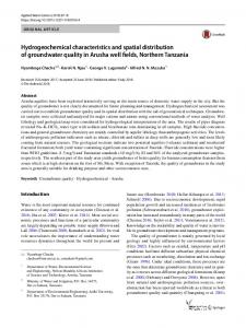
The study area was the Babaohe River Basin, which is a subcatchment in the upper reaches of the Heihe River Basin, China’s second largest inland river basin. The elevation is from 3000 m to about 5000 m. Permafrost and glacier are distributed in this area, and snow prevails in winter (Li et al., 2009). Figure 1 shows the digital elevation model of the Babaohe River Basin.
Discussion Paper
2 Study area, model and data
Full Screen / Esc
Printer-friendly Version Interactive Discussion
8837
|
Discussion Paper | Discussion Paper
25
HESSD 8, 8831–8864, 2011
Spatial horizontal correlation characteristics X. Han et al.
Title Page Abstract
Introduction
Conclusions
References
Tables
Figures
J
I
J
I
Back
Close
|
20
Discussion Paper
15
|
10
Discussion Paper
5
projected into Longitude-Latitude Projection using MRT (MODIS Reprojection Tool). Then the MODIS PFT (12 types) was translated to CLM PFT (17 types) using the 1km global climate data WorldClim (Hijmans et al., 2005) and the methods proposed by (Bonan et al., 2002). The mean temperature of warmest season, mean temperature of coldest season, annual precipitation, precipitation of driest season, precipitation of warmest season and precipitation of coldest season data were taken from the World◦ Clim database. The growing-degree days above 5 C were calculated from the GLDAS forcing data we used in this study. These data were combined to reclassify the MODIS PFT to the CLM PFT based on the climate rules proposed by Bonan et al., 2002, and the fraction of each PFT type at each grid cell was calculated using the 4 MODIS grids contained in one CLM grid. The 4-day MODIS leaf area index (LAI) data (MCD15A3) at 1km resolution was used to calculate the monthly LAI, and the stem area index (SAI) was estimated based on the methods proposed by Lawrence and Chase (2007). In CLM, the soil color determines dry and saturated soil albedo. The soil thermal and hydraulic properties are estimated from sand, clay, and organic matter content. The maximum fractional saturated area is used to determine surface runoff and infiltration. The 1 km soil color data was calculated with help of the method of Lawrence and Chase, 2007, and the soil texture data. The soil sand fraction, clay fraction, organic matter density and soil bulk density are from the Harmonized World Soil Database ˙ v1.1 (HWSD) (FAO et al., 2009). The HWSD is a 30arc-s raster database with over 16 000 different soil mapping units that combines existing regional and national updates of soil information worldwide (SOTER, ESD, Soil Map of China, WISE) with the information contained within the 1:5 000 000 scale FAO-UNESCO Soil Map of the World. The maximum fractional saturated area, which is defined as the cumulative distribution function (CDF) of the topographic index when the grid cell mean water table depth is zero, was calculated based on the methods proposed by Niu et al. (2005) using the 100 m GDEM (GDEM is a product of METI and NASA) and 1 km SRTM DEM (Jarvis et al., 2008).
Full Screen / Esc
Printer-friendly Version Interactive Discussion
3.1 Experiment design
5
Discussion Paper |
8838
|
25
The presence of horizontal spatial dependence of land surface properties is typically identified using geostatistical methods such as semivariogram analysis (Goovaerts, 1997; Ryu and Famiglietti, 2006). Several semivariogram models are often used to characterize the spatial dependence such as the Gaussian model, the exponential
Discussion Paper
3.2 Spatial horizontal correlation and geostatistics
HESSD 8, 8831–8864, 2011
Spatial horizontal correlation characteristics X. Han et al.
Title Page Abstract
Introduction
Conclusions
References
Tables
Figures
J
I
J
I
Back
Close
|
20
Discussion Paper
15
|
10
The Observing System Simulation Experiments (OSSE) were designed to evaluate the proposed methods. We run CLM for the complete years of 2007 and 2008 separately in hourly step. The surface soil moisture and surface temperature results at 11 September 2008, 06, calculated by CLM, were selected as the ground truth, which are shown in Fig. 2a and c, respectively. The surface soil moisture and surface temperature results at 11 September 2007, 06 were selected to be used as the model values that will be updated. Because the observation errors were spatially correlated, a spatially correlated Gaussian random field with mean 0.0 and an exponential semivariogram model with nugget 0.0, variance 0.0016 (i.e., the standard deviation of soil moisture observation is 0.04 (Vol/Vol), which is the volumetric accuracy of SMAP mission (Entekhabi et al., 2010)), and range 10 000.0 m was added to the true surface soil moisture data in order to obtain the synthetic surface soil moisture observation data. A second spatially correlated Gaussian random field with an exponential semivariogram model with mean 2 2 0.0 K, nugget 0.0 K , variance 1.0 K (i.e., the standard deviation of surface temperature observation is 1.0 K, which is the accuracy of MODIS land surface temperature product; Wan et al., 2004) and range 10 000.0 m was added to the true surface temperature data in order to obtain the synthetic surface temperature observation data. The random fields were generated using the geoR package (Ribeiro Jr and Diggle, 2001) of the statistical data analysis software R (http://www.r-project.org/).
Discussion Paper
3 Methodology
Full Screen / Esc
Printer-friendly Version Interactive Discussion
5
γ(h) = c0 + c(h/a ∗ (1.5 − 0.5 ∗ (h/a)2 ))
exponential
γ(h) = c0 + c(
matern
(4)
|
8839
Discussion Paper
where c0 is nugget, c is sill minus nugget, h is the separation distance, a is the correlation range, Kv is a modified Bessel function of the second kind of order v, Γis the gamma function and v(κ) is called “smoothness parameter” (v > 0). The normalized semivariogram γ(h)Nor is defined as γ(h)Nor = γ(h)/(c0 +c) and the correlogram is then given by 1 − γ(h)Nor . The nugget value describes the unresolved variance at the scale smaller than the smallest lag distance whereas the sill describes the variance of the observed data as they become spatially independent. The calculated correlogram needs be normalized using the maximum correlogram value, which means that the correlogram value is equal to one at the observation location. It gradually reduces towards 0.0 as the distance from the analysis grid cell increases, and is null beyond the specified correlation range. While there are K observations available during the analysis, the observation selection scheme in LETKF is as follows: spatial correlations between the observations and the model grid cell are calculated according to the model correlogram; the observations whose correlations are larger than a predefined threshold are selected for each model grid cell.
|
20
2v 1/2 h 2v 1/2 h v 1 ( ) Kv ( )) a a 2v−1 Γ(v)
(3)
Discussion Paper
15
Gaussian
HESSD 8, 8831–8864, 2011
Spatial horizontal correlation characteristics X. Han et al.
Title Page Abstract
Introduction
Conclusions
References
Tables
Figures
J
I
J
I
Back
Close
|
10
(2)
Discussion Paper
γ(h) = c0 + c(1 − exp(−(3h2 /a2 )))
(1)
|
γ(h) = c0 + c(1 − exp(−3h/a))
spherical
Discussion Paper
model, the spherical model and the matern model (Goovaerts, 1997; Minasny and McBratney, 2005). In this analysis, we only used these semivariogram models to characterize the spatial dependence of surface soil moisture and surface temperature. The models are defined as follows:
Full Screen / Esc
Printer-friendly Version Interactive Discussion
Discussion Paper |
8840
|
25
The local ensemble transform Kalman filter (LETKF) proposed by Hunt et al. (2007) is a new variant of the ensemble Kalman filter (EnKF). Compared with the various kinds of implementations of EnKF, such as stochastic EnKF (Burgers et al., 1998), deterministic methods (Whitaker and Hamill, 2002), the ensemble adjustment Kalman filter (EAKF) (Anderson, 2001), the ensemble transform Kalman filter (ETKF) (Bishop and Toth, 2001), and the Ensemble Square Root Filter (EnSRF) by Whitaker and Hamill (2002), the LETKF used a local analysis scheme (Houtekamer and Mitchell, 1998; Hunt et al., 2007; Kalnay et al., 2007; Miyoshi and Yamane, 2007; Whitaker et al., 2008).
Discussion Paper
20
HESSD 8, 8831–8864, 2011
Spatial horizontal correlation characteristics X. Han et al.
Title Page Abstract
Introduction
Conclusions
References
Tables
Figures
J
I
J
I
Back
Close
|
3.3 Local ensemble transform Kalman filter
Discussion Paper
15
|
10
Discussion Paper
5
In order to represent the vegetation or cloud cover impacts on the observation data, we extracted the valid grid cells from the MODIS land surface temperature product of Terra (MOD11A1- Daytime) from 4 February 2008. In the assimilation experiments, it is assumed that for the same grid cells meaningful remote sensing information is available, whereas for the other grid cells due to cloud cover and vegetation no meaningful information could be extracted. The position of the extracted valid grid cells are used as the mask and the synthetic observation data located at these grids were selected as the observation data to be assimilated. The surface soil moisture and surface temperature observation data used in the assimilation experiments are shown in Fig. 2b and d, respectively. In total 2618 valid observation grid cells were selected covering 72 percent of the model grid cells of this region. There are 1022 uncovered model grid cells without observations. The maximum distance considered when fitting the semivariogram was set as 10 000.0 m and pairs of locations with separation distances larger than this value were ignored. Then we fitted isotropic semivariograms of surface soil moisture and surface temperature observations for 2618 grid cells (the grid cells covered by remote sensing) and 3640 grid cells (all grid cells) using the geoR package in R and the best fitted semivariograms are shown in Fig. 3a, b, c and d, respectively. The fitted semivariograms model parameters are shown in Table 1.
Full Screen / Esc
Printer-friendly Version Interactive Discussion
i = 1,2,...,K
|
b(i ) Yb[g] = y [g] − y¯ b[g] ,
b 1. Average the vectors {x[g] } to get the m[g] dimensional vector x¯ [g] of the mean
ensemble value of the model predictions, then subtract this vector from each
b(i ) x[g]
to form the columns of the m[g] × k matrix Xb[g] which represents the deviation of the model given quantity from the ensemble mean (analogously to the quantity in point 1, but) for all the grid points.
|
8841
Discussion Paper
b(i )
20
Discussion Paper
b(i )
y [g] = H[g] × x[g]
HESSD 8, 8831–8864, 2011
Spatial horizontal correlation characteristics X. Han et al.
Title Page Abstract
Introduction
Conclusions
References
Tables
Figures
J
I
J
I
Back
Close
|
b
from each {y [g] } to form the columns of the l[g] × k matrix Y[g] , which represents the deviation of the given quantity of each ensemble component from the mean ensemble value, in each point where an observation exists. b(i )
Discussion Paper
b(i )
15
|
10
Discussion Paper
5
The spatial correlation characteristics of the observations were introduced in the framework of the LETKF local analysis scheme. The input to the LETKF is given by the number of simulations with varying parameters, i.e. the ensembles number k; a backb(i ) ground ensemble of m[g] dimensional model state vectors{x[g] : i = 1,2,...,k}, where the subscript gmeans the inputs hold the global model state with m[g] coinciding in a o gridded model with the number of grid cells; an l[g] dimensional observation vector y [g] ; the observation operator H[g] map the m[g] dimensional model space into the l[g] < m[g] observation space; and an l[g] × l[g] dimensional observation error covariance matrix R[g] . The analysis scheme is as follows (Hunt et al., 2007): b(i ) b(i ) Apply the H[g] to each model state x[g] to get the global background ensemble y [g] , i.e. the first guess of the quantities to be explored, as derived from the model run at a time step, in the points where measurements are available. Average the latter vectors over the ensembles to get the l[g] dimensional vector y¯ b[g] . Then subtract this vector
Full Screen / Esc
Printer-friendly Version Interactive Discussion
2. For each of the grid cell and the observations with a correlation larger than a threshold value were selected. b T
5
−1
a
˜ 5. Compute the k × k matrix W = [(k − 1)P] 10
˜ a C(y o − y¯ b ), and add it to each column 6. Compute the k dimensional vector w¯ = P a of W a(i )
b
b
= x¯ + X ∗ w
a(i )
, i = 1,2,...,K
Discussion Paper
Based on the equations given, the local analysis scheme is performed. It only considers the observations located in a local region surrounding the analysis grid cell. The observations are selected for each grid cell. The grid cell by grid cell analysis method can easily be parallelized and is useful to decrease the computational burden for the large scale data assimilation.
|
3.4 Ensemble generation Because we run the model once and we have only one model value. The model ensemble members of surface soil moisture and surface temperature, necessary as input for the LETKF algorithm are obtained using the additive perturbation method (Constantinescu et al., 2007; Corazza et al., 2003). The model forecast errors are modeled by a geostatistical model and the model ensemble members are generated by geostatistical stochastic realizations. The ensemble members are generated as follows:
|
8842
Discussion Paper
20
HESSD 8, 8831–8864, 2011
Spatial horizontal correlation characteristics X. Han et al.
Title Page Abstract
Introduction
Conclusions
References
Tables
Figures
J
I
J
I
Back
Close
|
7. x
15
1/2
Discussion Paper
˜ a = [(k − 1)I + CYb ]−1 4. Compute the k × k matrix P
|
3. Compute the k × l matrix C = (Y ) R × r, where r is a correlation function that gradually reduces towards zero as the distance from the analysis grid cell increases. r is given by the geostatistically determined correlogram.
Discussion Paper
b(i )
Xb[g] = x[g] − x¯ b[g] , i = 1,2,...,K
Full Screen / Esc
Printer-friendly Version Interactive Discussion
5
| Discussion Paper
25
|
Three assimilation strategies were evaluated: (Strategy-1) Only the covered grid cells (2618) were updated; (Strategy-2) All grid cells with sufficient correlated observations in the neighborhood were updated, it means almost 3640 grids were updated (depends on the availability of valid correlated observations), the uncovered grid cells were updated using the observations within a local window, and the model grids without sufficiently correlated observations were not updated; (Strategy-3) We assumed 8843
Discussion Paper
3.5 Data assimilation strategies
HESSD 8, 8831–8864, 2011
Spatial horizontal correlation characteristics X. Han et al.
Title Page Abstract
Introduction
Conclusions
References
Tables
Figures
J
I
J
I
Back
Close
|
20
Discussion Paper
15
where Yn (i ,j ) is the n-th ensemble member of the model forecast at row i and column j of the computational grid. Y (i ,j ) is the model forecast value, ωn (i ,j ) is the n-th ensemble member drawn from a mean-zero stationary Gaussian space-time stochastic process and it represents the model forecast error. First we calculated the model forecast errors by subtracting the model forecast from the true reference for surface soil moisture and surface temperature, respectively. Next, the semivariograms of model forecast errors for surface soil moisture and surface temperature were fitted using the geoR package in R and are shown in Fig. 4a and b, respectively. The best fitted semivariogram model for model forecast error of surface soil moisture is the matern model with nugget 5.103e-05, sill 6.124e-4, kappa 1.0 and range 3057.51 m. The best fitted semivariogram model for model forecast error of 2 2 surface temperature is the exponential model with nugget 1.535 K , sill 15.943 K and range 4828.21 m. The stationary Gaussian random fields of the residuals of surface soil moisture and surface temperature were generated using the grf method in geoR package with the fitted semivariograms in Fig. 4a and b, respectively. 100 ensemble members of forecast error were generated, and then added Y (i ,j ) to obtain the surface soil moisture and surface temperature model ensembles, respectively. The ensemble members were generated once and served then as input to LETKF for data assimilation.
|
10
(5)
Discussion Paper
Yn (i ,j ) = Y (i ,j ) + ωn (i ,j )
Full Screen / Esc
Printer-friendly Version Interactive Discussion
Discussion Paper |
8844
|
In order to evaluate the quality of the obtained results, the Root Mean Square Error (RMSE) and Nash-Sutcliffe model efficiency (NSE) coefficient were calculated according to: q RMSE = mean[(Estimated-Truth)2 ] (6)
Discussion Paper
20
HESSD 8, 8831–8864, 2011
Spatial horizontal correlation characteristics X. Han et al.
Title Page Abstract
Introduction
Conclusions
References
Tables
Figures
J
I
J
I
Back
Close
|
4 Results
Discussion Paper
15
|
10
Discussion Paper
5
the observations at all grid cells were available, no vegetation or cloud cover existed (i.e., 3640 grid cells were covered). For each strategy, there are 4 local observation selection options to integrate the correlated observations into the analysis scheme: (1) Only 1 observation was used for each grid cell (1-Obs); (2) No more than 4 observations were used for each grid cell (4-Obs); (3) No more than 9 observations were used for each grid cell (9-Obs); (4) No more than 16 observations were used for each grid cell (16-Obs). Figure 5 summarizes the data assimilation procedure including the different strategies (Strategy-1 and Strategy-2). The selection of observations to be used for each model grid cell depends upon the observations’ correlation characteristics. As explained before, the observations are selected as function of the distance dependent correlation fitted with help of the correlogram. It should be noted that some of the observations used in the analysis at one grid cell are also used in the analysis of another neighboring grid cell. This imposes a smoothing effect from one grid cell to the next. The threshold value was defined as 0.001; it means that all the observations with correlogram larger than 0.001 were considered. The selected observations were sorted in descending order according to the correlogram values and no more than 1, 4, 9 or 16 of them were selected.
Full Screen / Esc
Printer-friendly Version Interactive Discussion
NSE = 1 − P
Discussion Paper |
8845
|
25
Discussion Paper
20
HESSD 8, 8831–8864, 2011
Spatial horizontal correlation characteristics X. Han et al.
Title Page Abstract
Introduction
Conclusions
References
Tables
Figures
J
I
J
I
Back
Close
|
15
where the estimated value was the model value or the assimilation value, respectively. N is the number of active grid cells, it is 3640 in this case. The smaller the RMSE value and the larger the NSE value, the better the assimilation results. Table II shows the RMSE and NSE for surface soil moisture. From Table 2, we can see that the best surface soil moisture assimilation result for each Strategy is 16-Obs. The best results are obtained for the simulation scenario 16-Obs of Strategy-3, where the observations cover the whole region. The RMSE value decreases 30.1 percent and the NSE value is 4.0 times larger if compared with a scenario without data assimilation. If the observation data only cover 72 percent of the whole region, the best result is for the simulation scenario 16-Obs of Strategy-2. The RMSE value decreases 29.4 percent and the NSE value is 3.9 times larger compared with the case without data assimilation. The differences between the results of Strategy (1) and the results of Strategy (2) show the improvement at the grid cells without direct observations. Compared with Strategy-1, the RMSE values of Strategy-2 decrease 3.2, 6.6, 7.7 and 8.1 percent for 1-Obs, 4-Obs, 9-Obs and 16-Obs, respectively. NSE values of Strategy-2 are 0.42, 0.80, 0.91 and 0.94 times larger for 1-Obs, 4-Obs, 9-Obs and 16-Obs, respectively. For each case, the increased number of observations used in the LETKF can improve the estimation, with lower RMSE values and increased NSE value. We had 2618 observations in both Strategy-1 and Strategy-2, Strategy-2 performed better than Strategy-1 after the incorporation of the spatial horizontal correlation. In Strategy-2, the RMSE (NSE) values decrease (increase) 10.5 (33.4) percent from 1-Obs to 4-Obs, and RMSE (NSE) values decrease 4.6 (8.9) percent from 4-Obs to 9-Obs, and RMSE (NSE) values decrease 1.6 (2.6) percent from 9-Obs to 16-Obs in Strategy-2. Although the scheme of 16-Obs used 7 additional observations for each grid cell as compared to 9-Obs, the results did not improve much further. Incorporating 9 correlated observations is enough for surface soil moisture assimilation in this case.
Discussion Paper
10
(7)
N 2 n=1 [Truth-mean(Truth)]
|
5
n=1 (Estimated-Truth)
Discussion Paper
PN
Full Screen / Esc
Printer-friendly Version Interactive Discussion
8846
|
Discussion Paper | Discussion Paper
25
HESSD 8, 8831–8864, 2011
Spatial horizontal correlation characteristics X. Han et al.
Title Page Abstract
Introduction
Conclusions
References
Tables
Figures
J
I
J
I
Back
Close
|
20
Discussion Paper
15
|
10
Discussion Paper
5
The best surface soil moisture results of Strategy-1, Strategy-2 and Strategy-3 are shown in Fig. 6b, c and d, respectively. The comparison of the spatial patterns for the truth and the different strategies shows again that Strategy-3 gives the best results, followed by Strategy-2 and Strategy-1. Table 3 shows the RMSE and NSE of surface temperature results. From Table III, we can see that the best surface soil temperature assimilation results for Strategy-1 and Strategy-3 are obtained if only one observation was assimilated. The best result of Strategy-2 is the scenario of 4-Obs. Strategy-3, where the observation data can cover the whole region, gives the best results with a decrease of the RMSE value of 91.4 percent and the NSE value is 7.2 times larger compared with the case without data assimilation. If the observation data only cover 72 percent of the whole region, results are better for Strategy-2 than the results for Strategy-1. The RMSE value is 54.5 percent lower and the NSE value is 5.8 times larger compared with the case without data assimilation. Results for soil temperature are similar to results for surface soil moisture: the surface temperature estimations at the uncovered region can be improved by the correlated observations. The differences between the results of Strategy-1 and the results of Strategy-2 can show the improvement at the grid cells without direct observations. Compared with Strategy-1, the RMSE values of Strategy-2 decrease 30.3, 33.7, 32.6 and 30.1 percent for 1-Obs, 4-Obs, 9-Obs and 16-Obs, respectively. NSE values of Strategy-2 are 2.68, 2.93, 2.87 and 2.73 times larger for 1-Obs, 4-Obs, 9-Obs and 16-Obs, respectively. For Strategy-1 and Strategy-3, the increased number of observations used in the LETKF yielded increased RMSE values and decreased NSE values for soil temperature characterization. Incorporating more observations did not improve the results further in the surface temperature assimilation; one of the most correlated observations will be enough for the covered grid cells. On the other hand, in the 4-Obs and 9-Obs scenarios of Strategy-2, the increased number of observations improved the assimilation results. Therefore, for the uncovered grid cells the use of several observations improves the estimations as compared with only one observation.
Full Screen / Esc
Printer-friendly Version Interactive Discussion
5
Discussion Paper
The best surface temperature results of Strategy-1, Strategy-2 and Strategy-3 are shown in Fig. 7b, c and d, respectively. The comparison of the spatial patterns for the reference field (“truth”) and the different strategies leads to conclusions, which are consistent with the comparison of the RMSE and NSE statistics. 5 Summary and discussion
|
8847
|
| Discussion Paper
25
Discussion Paper
20
8, 8831–8864, 2011
Spatial horizontal correlation characteristics X. Han et al.
Title Page Abstract
Introduction
Conclusions
References
Tables
Figures
J
I
J
I
Back
Close
|
15
Discussion Paper
10
We carried out a set of synthetic observing system simulation experiments to explicitly include the spatial correlation characteristics of observations in the land data assimilation for actualizing surface soil moisture and soil temperature at locations without remote sensing observations. Two different spatial correlation schemes were evaluated: (1) For the grid cells covered with observations, additional observations around the grid cells were included in the data assimilation; (2) For the grid cells without observations, observations surrounding these grid cells were used. Firstly, we characterized the spatial horizontal correlation of the observations on the basis of a semivariogram analysis. The selected semivariogram models and the derived correlogram values were used to choose the correlated observations for each model grid in LETKF during assimilation. The selected observations were sorted according to the correlogram values and the simulation experiments considered different numbers of observations to be used in the data assimilation. The surface soil moisture results showed that the estimation can be improved when for a certain grid cell surrounding observations were included in the estimation. The estimations at the uncovered grid cells were also improved when the surrounding correlated observations were used, and the more observations, the better the results, but more than nine observations of soil moisture did not improve much the estimation in this case. The results for surface temperature assimilation also showed that the estimation can be improved when for a certain grid cell surrounding observations were included in the estimation. For the covered grid cells, more observations will not improve the
HESSD
Full Screen / Esc
Printer-friendly Version Interactive Discussion
| Discussion Paper |
8848
Discussion Paper
25
HESSD 8, 8831–8864, 2011
Spatial horizontal correlation characteristics X. Han et al.
Title Page Abstract
Introduction
Conclusions
References
Tables
Figures
J
I
J
I
Back
Close
|
20
Discussion Paper
15
|
10
Discussion Paper
5
estimations, and one of the most correlated observations is enough to obtain the best estimation. The estimations at the uncovered grid cells could be improved when the surrounding correlated observations were used and including more observations yielded better results. These results indicated that the correlated surface temperature observations can improve the assimilation results. Our study showed that including the horizontal spatial dependence of surface soil moisture and surface temperature observations in the data assimilation scheme improved the prediction. The model estimations at the grid cells without the observations can be improved using the geostatistical model and LETKF. We also evaluated the proposed methods in different time periods and obtained similar results. However, the ensemble generation method that we used is different from the usual approaches. The uncertainties of different sources were not considered explicitly. We perturbed the model simulation results instead. In addition to including spatial dependence of observed state variables, it may be worthwhile to also include temporal dependence of land surface observations in data assimilation schemes for an improved estimation of state variables. Experimental data clearly shows that land surface variables, such as soil moisture and soil temperature are correlated in time. Temporal stability of soil moisture (Brocca et al., 2010; De Lannoy et al., 2006) has been extensively studied. Dunne and Entekhabi (2005) studied the ensemble Kalman smoother in the soil moisture assimilation, but temporal correlation potential has not yet been fully explored in the framework of data assimilation schemes. Moreover, land cover and soil type-dependent spatial horizontal correlations may improve the findings of this study. An operational application of the presented spatial horizontal correlation patterns may be feasible also for the assimilation of surface soil moisture and surface temperature in weather forecast models like the ECMWF Integrated Forecast System (Drusch et al., 2009).
Full Screen / Esc
Printer-friendly Version Interactive Discussion
Discussion Paper |
8849
|
30
Discussion Paper
25
HESSD 8, 8831–8864, 2011
Spatial horizontal correlation characteristics X. Han et al.
Title Page Abstract
Introduction
Conclusions
References
Tables
Figures
J
I
J
I
Back
Close
|
20
Anderson, J. L.: An ensemble adjustment Kalman filter for data assimilation, Mon. Weather Rev., 129, 2884–2903, 2001. Anterrieu, E.: On the Detection and Quantification of RFI in L1a Signals Provided by SMOS, IEEE T. Geosci. Remote Sens., 1–7, 2011. Bishop, C. H., Toth, Z., Etherton, B. J., and Majumdar, S. J.: Adaptive sampling with the ensemble transform Kalman filter, Part I: Theoretical aspects, Mon. Weather Rev., 129, 420–436, 2001. Bonan, G. B., Levis, S., Kergoat, L., and Oleson, K. W.: Landscapes as patches of plant functional types: An integrating concept for climate and ecosystem models, Global Biogeochem. Cy., 16, 1021, doi:10.1029/2000GB001360, 2002. Brocca, L., Melone, F., Moramarco, T., and Morbidelli, R.: Spatial-temporal variability of soil moisture and its estimation across scales, Water Resour. Res., 46, W02516, doi:10.1029/2009WR008016, 2010. Burgers, G., van Leeuwen, P. J., and Evensen, G.: Analysis scheme in the ensemble Kalman filter, Mon. Weather Rev., 126, 1719–1724,1998. Chen, F., Crow, W. T., Starks, P. J., and Moriasi, D. N.: Improving hydrologic predictions of a catchment model via assimilation of surface soil moisture, Adv. Water Resour., 34, 526– 536,2011. Chiles, J. P. and Delfiner, P.: Geostatistics: modeling spatial uncertainty, Wiley-Interscience, 1999.
Discussion Paper
15
References
|
10
Discussion Paper
5
Acknowledgements. This work was supported by the Knowledge Innovation Program of the Chinese Academy of Sciences (grant number: KZCX2-EW-312), the NSFC (National Science Foundation of China) project (grant number: 40901160, 40925004) and the National Basic Research Program of China (973 Program) (grant number: 2009CB421305). Carsten Montzka received financial support from the DFG (German Science foundation) by means of the project TR-32 “Patterns in Soil-Vegetation-Atmosphere systems: Monitoring, modeling and data assimilation”, which is gratefully acknowledged. The data used in this study were acquired as part of the mission of NASA’s Earth Science Division and archived and distributed by the Goddard E arth Sciences (GES) Data and Information Services Center (DISC).
Full Screen / Esc
Printer-friendly Version Interactive Discussion
8850
|
| Discussion Paper
30
Discussion Paper
25
HESSD 8, 8831–8864, 2011
Spatial horizontal correlation characteristics X. Han et al.
Title Page Abstract
Introduction
Conclusions
References
Tables
Figures
J
I
J
I
Back
Close
|
20
Discussion Paper
15
|
10
Discussion Paper
5
Coll, C., Wan, Z., and Galve, J. M.: Temperature-based and radiance-based validations of the V5 MODIS land surface temperature product, J. Geophys. Res.-Atmos., 114, D20102, doi:10.1029/2009JD012038, 2009. Constantinescu, E. M., Sandu, A., Chai, T., and Carmichael, G. R.: Ensemble-based chemical data assimilation. I: General approach, Q. J. Roy. Meteorol. Soc., 133, 1229–1243, 2007. Corazza, M., Kalnay, E., Patil, D. J., Yang, S.-C., Morss, R., Cai, M., Szunyogh, I., Hunt, B. R., and Yorke, J. A.: Use of the breeding technique to estimate the structure of the analysis “errors of the day”, Nonlin. Processes Geophys., 10, 233–243, doi:10.5194/npg-10-233-2003, 2003. Crow, W. T., Kustas, W. P., and Prueger, J. H.: Monitoring root-zone soil moisture through the assimilation of a thermal remote sensing-based soil moisture proxy into a water balance model, Remote Sens. Environ., 112, 1268–1281, 2008. Crow, W. T. and Van Loon, E.: Impact of incorrect model error assumptions on the sequential assimilation of remotely sensed surface soil moisture, J. Hydrometeorol., 7, 421–432, 2006. Dai, Y., Zeng, X., Dickinson, R. E., Baker, I., Bonan, G. B., Bosilovich, M. G., Denning, A. S., Dirmeyer, P. A., Houser, P. R., Niu, G., Schlosser, A., and Yang, Z. L.: The common land model, B. Am. Meteorol. Soc., 84, 1013–1024, 2003. De Lannoy, G. J. M., Verhoest, N. E. C., Houser, P. R., Gish, T. J., and Van Meirvenne, M.: Spatial and temporal characteristics of soil moisture in an intensively monitored agricultural field (OPE(3)), J. Hydrol., 331, 719–730,2006. Dorigo, W. A., Scipal, K., Parinussa, R. M., Liu, Y. Y., Wagner, W., de Jeu, R. A. M., and Naeimi, V.: Error characterisation of global active and passive microwave soil moisture datasets, Hydrol. Earth Syst. Sci., 14, 2605–2616, doi:10.5194/hess-14-2605-2010, 2010. Draper, C. S., Mahfouf, J. F., and Walker, J. P.: Root zone soil moisture from the assimilation of screen-level variables and remotely sensed soil moisture, J. Geophys. Res.-Atmos., 116, D02127, doi:10.1029/2010JD013829, 2010. Drusch, M., Scipal, K., de Rosnay, P., Balsamo, G., Andersson, E., Bougeault, P., and Viterbo, P.: Towards a Kalman Filter based soil moisture analysis system for the operational ECMWF Integrated Forecast System, Geophys. Res. Lett., 36, L10401, doi:10.1029/2009GL037716, 2009. Dunne, S. and Entekhabi, D.: An ensemble-based reanalysis approach to land data assimilation, Water Resour. Res, 41, W02013, doi:10.1029/2004WR003449, 2005.
Full Screen / Esc
Printer-friendly Version Interactive Discussion
8851
|
| Discussion Paper
30
Discussion Paper
25
HESSD 8, 8831–8864, 2011
Spatial horizontal correlation characteristics X. Han et al.
Title Page Abstract
Introduction
Conclusions
References
Tables
Figures
J
I
J
I
Back
Close
|
20
Discussion Paper
15
|
10
Discussion Paper
5
Entekhabi, D., Njoku, E. G., O’Neill, P. E., Kellogg, K. H., Crow, W. T., Edelstein, W. N., Entin, J. K., Goodman, S. D., Jackson, T. J., Johnson, J., Kimball, J., Piepmeier, J. R., Koster, R. D., Martin, N., McDonald, K. C., Moghaddam, M., Moran, S., Reichle, R., Shi, J. C., Spencer, M. W., Thurman, S. W., Tsang, L., and Van Zyl, J.: The Soil Moisture Active Passive (SMAP) Mission,Proceedings Of The Ieee, 98, 704–716, 2010. FAO, IIASA, ISRIC, ISSCAS, and JRC: Harmonized World Soil Database (version 1.1), In. FAO, Rome, Italy and IIASA, Laxenburg, Austria, 2009. Flores, A. N., Ivanov, V. Y., Entekhabi, D., and Bras, R. L.: Impact of hillslope-scale organization of topography, soil moisture, soil temperature, and vegetation on modeling surface microwave radiation emission, IEEE T. Geosci. Remote Sens., 47, 2557–2571, 2009. Ghent, D., Kaduk, J., Remedios, J., Ardo, J., and Balzter, H.: Assimilation of land surface temperature into the land surface model JULES with an ensemble Kalman filter, J. Geophys. Res.-Atmos., 115, D19112, doi:10.1029/2010JD014392, 2010. Goovaerts, P.: Geostatistics for natural resources evaluation,Oxford University Press, USA, 1997. Greybush, S. J., Kalnay, E., Miyoshi, T., Ide, K., and Hunt, B. R.: Balance and Ensemble Kalman Filter Localization Techniques, Mon. Weather Rev., 139, 511–522, 2010. Hijmans, R. J., Cameron, S. E., Parra, J. L., Jones, P. G., and Jarvis, A.: Very high resolution interpolated climate surfaces for global land areas, Int. J. Climatol., 25, 1965–1978,2005. Houtekamer, P. L. and Mitchell, H. L.: Data Assimilation Using an Ensemble Kalman Filter Technique, Mon. Weather Rev., 126, 796–811,1998. Hunt, B. R., Kostelich, E. J., and Szunyogh, I.: Efficient data assimilation for spatiotemporal chaos: A local ensemble transform Kalman filter, Physica D, 230, 112–126, 2007. Jarvis, A., Reuter, H. I., Nelson, A., and Guevara, E.: Hole-filled seamless SRTM data V4, International Centre for Tropical Agriculture, 2008. Kalnay, E., Li, H., Miyoshi, T., YANG, S.H.U.C., and BALLABRERA-POY, J.: 4-D-Var or ensemble Kalman filter, Tellus, 59, 758–773, 2007. Kerr, Y. H., Waldteufel, P., Wigneron, J. P., Delwart, S., Cabot, F., Boutin, J., Escorihuela, M. J., Font, J., Reul, N., Gruhier, C., Juglea, S. E., Drinkwater, M. R., Hahne, A., Martin-Neira, M., and Mecklenburg, S.: The SMOS Mission: New Tool for Monitoring Key Elements ofthe Global Water Cycle, Proceedings Of The IEEE, 98, 666–687, 2010.
Full Screen / Esc
Printer-friendly Version Interactive Discussion
8852
|
| Discussion Paper
30
Discussion Paper
25
HESSD 8, 8831–8864, 2011
Spatial horizontal correlation characteristics X. Han et al.
Title Page Abstract
Introduction
Conclusions
References
Tables
Figures
J
I
J
I
Back
Close
|
20
Discussion Paper
15
|
10
Discussion Paper
5
Lakhankar, T., Jones, A. S., Combs, C. L., Sengupta, M., Haar, T., and Khanbilvardi, R.: Analysis of Large Scale Spatial Variability of Soil Moisture Using a Geostatistical Method, SENSORS, 10, 913–932, 2010. Lawrence, P. J. and Chase, T. N.: Representing a new MODIS consistent land surface in the Community Land Model (CLM 3.0), J. Geophys. Res.-Biogeosci., 112, G01023, doi:10.1029/2006JG000168, 2007. Li, X., Huang, C. L., Che, T., Jin, R., Wang, S. G., Wang, J. M., Gao, F., Zhang, S. W., Qiu, C. J., and Wang, C. H.: Development of a Chinese land data assimilation system: its progress and prospects, Prog. Nat. Sci., 17, 881–892, 2007. Li, X., Li, X. W., Li, Z. Y., Ma, M. G., Wang, J., Xiao, Q., Liu, Q., Che, T., Chen, E. X., Yan, G. J., Hu, Z. Y., Zhang, L. X., Chu, R. Z., Su, P. X., Liu, Q. H., Liu, S. M., Wang, J. D., Niu, Z., Chen, Y., Jin, R., Wang, W. Z., Ran, Y. H., Xin, X. Z., and Ren, H. Z.: Watershed Allied Telemetry Experimental Research, J. Geophys. Res.-Atmos., 114, D22103, doi:10.1029/2008JD011590, 2009. Liston, G. E. and Elder, K.: A meteorological distribution system for high-resolution terrestrial modeling (MicroMet), J. Hydrometeorol., 7, 217–234, 2006. Matzler, C. and Standley, A.: Relief effects for passive microwave remote sensing, Int. J. Remote Sens., 21, 2403–2412, 2000. McLaughlin, D., Zhou, Y. H., Entekhabi, D., and Chatdarong, V.: Computational issues for large-scale land surface data assimilation problems, J. Hydrometeorol., 7, 494–510, 2006. Minasny, B. and McBratney, A.B.: The Matern function as a general model for soil variograms, GeodermaPedometrics 2003, 128, 192–207, 2005. Miyoshi, T. and Yamane, S.: Local ensemble transform Kalman filtering with an AGCM at a T159/L48 resolution, Mon. Weather Rev., 135, 3841–3861, 2007. Montzka, C., Moradkhani, H., Weihermuller, L., Franssen, H., Canty, M., and Vereecken, H.: Hydraulic parameter estimation by remotely-sensed top soil moisture observations with the particle filter, J. Hydrol., 399, 410–421, 2011. Moradkhani, H.:Hydrologic remote sensing and land surface data assimilation, SENSORS, 8, 2986–3004, 2008. Naeimi, V., Scipal, K., Bartalis, Z., Hasenauer, S., and Wagner, W.: An improved soil moisture retrieval algorithm for ERS and METOP scatterometer observations, IEEE T. Geosci. Remote Sens., 47, 1999–2013, 2009.
Full Screen / Esc
Printer-friendly Version Interactive Discussion
8853
|
| Discussion Paper
30
Discussion Paper
25
HESSD 8, 8831–8864, 2011
Spatial horizontal correlation characteristics X. Han et al.
Title Page Abstract
Introduction
Conclusions
References
Tables
Figures
J
I
J
I
Back
Close
|
20
Discussion Paper
15
|
10
Discussion Paper
5
Niu, G. Y., Yang, Z. L., Dickinson, R. E., and Gulden, L. E.: A simple TOPMODEL-based runoff parameterization (SIMTOP) for use in global climate models, J. Geophys. Res.-Atmos., 110, D21106, doi:10.1029/2005JD006111, 2005. Njoku, E. G. and Chan, S. K.: Vegetation and surface roughness effects on AMSR-E land observations, Remote Sens. Environ., 100, 190–199, 2006. Oleson, K. W., Lawrence, D. M., Gordon, B., Flanner, M. G., Kluzek, E., Peter, J., Levis, S., Swenson, S. C., Thornton, E., Feddema, J., Heald, C. L., Hoffman, F., Lamarque, J.-F., Mahowald, N., Niu, G. Y., Qian, T., Randerson, J., Running, S., Sakaguchi, K., Slater, A., Stockli, R., Wang, A., Yang, Z.-L., Zeng, X., and Zeng, X.: Technical description of version 4.0 of the Community Land Model (CLM), NCAR Technical Note NCAR/TN-478+STR, National Center for Atmospheric Research, Boulder, CO, 257 pp. ,2010. Pan, M. and Wood, E.F.:Impact of Accuracy, Spatial Availability, and Revisit Time of SatelliteDerived Surface Soil Moisture in a Multiscale Ensemble Data Assimilation System,IEEE Journal of Selected Topics in Applied Earth Observations and Remote Sensing, 3, 49–56, 2010. Pellenq, J., Kalma, J., Boulet, G., Saulnier, G. M., Wooldridge, S., Kerr, Y., and Chehbouni, A.: A disaggregation scheme for soil moisture based on topography and soil depth, J. Hydrol., 276, 112–127, 2003. Pipunic, R. C., Walker, J. P., and Western, A.: Assimilation of remotely sensed data for improved latent and sensible heat flux prediction: A comparative synthetic study, Remote Sens. Environ., 112, 1295–1305, 2008. Reichle, R. H.: Data assimilation methods in the Earth sciences, Adv. Water Resour., 31, 1411–1418, 2008. Reichle, R. H., Kumar, S. V., Mahanama, S., Koster, R. D., and Liu, Q.: Assimilation of SatelliteDerived Skin Temperature Observations into Land Surface Models, J. Hydrometeorol., 11, 1103–1122, 2010. Reichle, R. H. and Koster, R. D.: Assessing the impact of horizontal error correlations in background fields on soil moisture estimation, J. Hydrometeorol., 4, 1229–1242,2003. Ribeiro Jr, P. J. and Diggle, P. J.:geoR: A package for geostatistical analysis, R news, 1, 14–18, 2001. Rodell, M., Houser, P. R., Jambor, U., Gottschalck, J., Mitchell, K., Meng, C. J., Arsenault, K., Cosgrove, B., Radakovich, J., Bosilovich, M., Entin, J. K., Walker, J. P., Lohmann, D., and Toll, D.:The global land data assimilation system, B. Am. Meteorol. Soc., 85, 381–394, 2004.
Full Screen / Esc
Printer-friendly Version Interactive Discussion
Discussion Paper | Discussion Paper |
8854
HESSD 8, 8831–8864, 2011
Spatial horizontal correlation characteristics X. Han et al.
Title Page Abstract
Introduction
Conclusions
References
Tables
Figures
J
I
J
I
Back
Close
|
20
Discussion Paper
15
|
10
Discussion Paper
5
Ryu, D. and Famiglietti, J. S.: Multi-scale spatial correlation and scaling behavior of surface soil moisture, Geophys. Res. Lett., 33, L08404, doi:10.1029/2006GL025831, 2006. Skou, N., Misra, S., Balling, J. E., Kristensen, S. S., and Sobjaerg, S. S.: L-band RFI as experienced during airborne campaigns in preparation for SMOS, IEEE T. Geosci. Remote Sens., 48, 1398–1407, 2010. Spadavecchia, L. and Williams, M.: Can spatio-temporal geostatistical methods improve high resolution regionalisation of meteorological variables?, Agric. Forest Meteorol., 149, 1105– 1117, 2009. Tian, X. J., Xie, Z. H., Dai, A. G., Jia, B. H., and Shi, C. X.: A microwave land data assimilation system: Scheme and preliminary evaluation over China, J. Geophys. Res.-Atmos., 115, D21113, doi:10.1029/2010JD014370, 2010. Turner, M. R. J., Walker, J. P., and Oke, P. R.: Ensemble member generation for sequential data assimilation, Remote Sens. Environ., 112, 1421–1433, 2008. Wan, Z., Zhang, Y., Zhang, Q., and Li, Z. L.: Quality assessment and validation of the MODIS global land surface temperature, Int. J. Remote Sens., 25, 261–274, 2004. Wan, Z. and Li, Z. L.: Radiance-based validation of the V5 MODIS land-surface temperature product, Int. J. Remote Sens., 29, 5373–5395, 2008. Whitaker, J. S., Hamill, T. M., Wei, X., Song, Y., and Toth, Z.: Ensemble data assimilation with the NCEP global forecast system, Mon. Weather Rev., 136, 463–482, 2008. Whitaker, J. S. and Hamill, T. M.:Ensemble data assimilation without perturbed observations, Mon. Weather Rev., 130, 1913–1925, 2002. Xu, T. R., Liu, S. M., Liang, S. L., and Qin, J.: Improving Predictions of Water and Heat Fluxes by Assimilating MODIS Land Surface Temperature Products into the Common Land Model, J. Hydrometeorol., 12, 227–244, 2011.
Full Screen / Esc
Printer-friendly Version Interactive Discussion
Discussion Paper |
Soil moisture grid cells 2618
3640
2618
3640
|
exponential 7.07836e-05 0.001479 4586.25 m
exponential 0.0 0.001525 3057.51 m
spherical 2.7536 241.27 282248.49 m
exponential 1.8227 23.55 9332.57 m
Discussion Paper
Model Nugget Sill Range
Surface temperature grid cells
Discussion Paper
Table 1. Fitted semivariogram models and parameters for the surface soil moisture and the surface temperature observations
| Discussion Paper |
8855
HESSD 8, 8831–8864, 2011
Spatial horizontal correlation characteristics X. Han et al.
Title Page Abstract
Introduction
Conclusions
References
Tables
Figures
J
I
J
I
Back
Close
Full Screen / Esc
Printer-friendly Version Interactive Discussion
Discussion Paper |
1-Obs
4-Obs
9-Obs
16-Obs
0.04145 0.04145 0.04145 0.11393 0.11393 0.11393
0.03614 0.03482 0.03417 0.32641 0.37469 0.39789
0.03387 0.03115 0.03070 0.40857 0.49966 0.51391
0.03294 0.02973 0.02924 0.44060 0.54417 0.55910
0.03260 0.02926 0.02880 0.45190 0.55841 0.57219
8, 8831–8864, 2011
Spatial horizontal correlation characteristics X. Han et al.
Title Page Abstract
Introduction
Conclusions
References
Tables
Figures
J
I
J
I
Back
Close
|
CLM
Discussion Paper
Table 2. Root Mean Square Error (RMSE) and Nash-Sutcliffe model efficiency (NSE) coefficient of surface soil moisture assimilation: Strategy-1-only covered grids were updated, Strategy2-all grids with sufficient correlated observations were updated, and Strategy-3-all grids are covered.
HESSD
Discussion Paper
Strategy-1 - RMSE Strategy-2 - RMSE Strategy-3 - RMSE Strategy-1 - NSE Strategy-2 - NSE Strategy-3 - NSE
| Discussion Paper |
8856
Full Screen / Esc
Printer-friendly Version Interactive Discussion
Discussion Paper |
CLM
4-Obs
9-Obs
16-Obs
3.64011 2.18386 0.41249 0.33284 0.75987 0.99143
3.67069 2.05178 0.74027 0.32159 0.78804 0.97241
3.69240 2.12941 0.86954 0.31354 0.77170 0.96193
3.71573 2.27082 1.01607 0.30484 0.74037 0.94802
8, 8831–8864, 2011
Spatial horizontal correlation characteristics X. Han et al.
Title Page Abstract
Introduction
Conclusions
References
Tables
Figures
J
I
J
I
Back
Close
|
1-Obs
Discussion Paper
Table 3. Root Mean Square Error (RMSE) and Nash-Sutcliffe model efficiency (NSE) coefficient of surface temperature assimilation: Strategy-1-only covered grids were updated, Strategy-2-all grids with sufficient correlated observations were updated, and Strategy-3-all grids are covered.
HESSD
4.79866 4.79866 4.79866 −0.15941 −0.15941 −0.15941
Discussion Paper
Strategy-1 - RMSE Strategy-2 - RMSE Strategy-3 - RMSE Strategy-1 - NSE Strategy-2 - NSE Strategy-3 - NSE
| Discussion Paper |
8857
Full Screen / Esc
Printer-friendly Version Interactive Discussion
Discussion Paper
HESSD 8, 8831–8864, 2011
| Discussion Paper
Spatial horizontal correlation characteristics X. Han et al.
Title Page Introduction
Conclusions
References
Tables
Figures
J
I
J
I
Back
Close
|
Abstract
Discussion Paper |
Fig. 1. Babaohe digital elevation model (DEM). Discussion Paper |
8858
Full Screen / Esc
Printer-friendly Version Interactive Discussion
Discussion Paper
HESSD 8, 8831–8864, 2011
| Discussion Paper
Spatial horizontal correlation characteristics X. Han et al.
Title Page Introduction
Conclusions
References
Tables
Figures
J
I
J
I
Back
Close
|
Abstract
Discussion Paper
535
Figure 2. The truth and observation of surface soil moisture and surface temperature,
|
8859
Discussion Paper
540
|
536
Fig. 2. truth and (a) observation soil surface temperature, respec537 The respectively: True surfaceof soilsurface moisture, (b) moisture Surface soiland moisture observation used tively:538 (a) True soil (c) moisture, (b) Surface soil(d) moisture observation used in assimilation, in surface assimilation, True surface temperature, Surface temperature observation (c) True temperature observation used in assimilation. 539 surface temperature and (d) Surface used in assimilation.
Full Screen / Esc
Printer-friendly Version Interactive Discussion
Discussion Paper
HESSD 8, 8831–8864, 2011
| Discussion Paper
Spatial horizontal correlation characteristics X. Han et al.
Title Page Introduction
Conclusions
References
Tables
Figures
J
I
J
I
Back
Close
|
Abstract
|
8860
Discussion Paper
546
|
5423. Experimental Figure 3. Experimental semivariogram and fitted semivariogram model of Fig. semivariogram and fitted semivariogram model of observations: (a) 2618 543cells of observations: 2618 grid cells of surface soil moisture observation, grid obsergrid surface soil(a) moisture observation, (b) 3640 grid cells of surface(b) soil3640 moisture 544 (c) 2618 cells grid soil moisture observation, (c) and 2618(d) grid cellsgrid of surface vation, gridcells cellsofofsurface surface temperature observation 3640 cells of surface temperature observation 545 temperature observation and (d) 3640 grid cells of surface temperature observation.
Discussion Paper
541
Full Screen / Esc
Printer-friendly Version Interactive Discussion
Discussion Paper
HESSD 8, 8831–8864, 2011
| Discussion Paper
Spatial horizontal correlation characteristics X. Han et al.
Title Page Introduction
Conclusions
References
Tables
Figures
J
I
J
I
Back
Close
|
Abstract
Discussion Paper
547 5484. Experimental Figure 4. Experimental semivariogram andsemivariogram fitted semivariogram of surface Fig. semivariogram and fitted modelmodel of surface soil soil moisture 549 moisture (a) and surface temperature (b). (a) and surface temperature (b). 550 551
| Discussion Paper |
8861
Full Screen / Esc
Printer-friendly Version Interactive Discussion
Discussion Paper
HESSD 8, 8831–8864, 2011
| Discussion Paper
Spatial horizontal correlation characteristics X. Han et al.
Title Page Introduction
Conclusions
References
Tables
Figures
J
I
J
I
Back
Close
|
Abstract
|
553 Figure 5. Flow chart of the Strategy-1 and Strategy-2: (Strategy-1) only the covered Fig. 5. Flow chart of the Strategy-1 and Strategy-2: (Strategy-1) only the covered grid cells 554 grid cells (2618) were updated; (Strategy-2) all grid cells with sufficient correlated (2618) were updated; (Strategy-2) all grid cells with sufficient correlated observations in the neighborhood were updated. 555 observations in the neighborhood were updated.
Discussion Paper
552
Discussion Paper
556 557 558
|
8862
Full Screen / Esc
Printer-friendly Version Interactive Discussion
Discussion Paper
559
HESSD 8, 8831–8864, 2011
| Discussion Paper
Spatial horizontal correlation characteristics X. Han et al.
Title Page Introduction
Conclusions
References
Tables
Figures
J
I
J
I
Back
Close
|
Abstract
Discussion Paper
560
Figure 6. The model ensemble mean of surface temperature and best assimilation
|
of 16-Obs in Stategy3.
Discussion Paper
561
Fig. 6. The model surface temperature and best assimilation results of different strategies: (a) 562 soil moisture results of different strategies: surface soil moisture of CLM ensemble surface of CLM, (b) the (a) result of 16-Obs in Stategy1, (c) themean, result(b)of 16-Obs in Stategy2 and (d) the result of 16-Obs in Stategy3. 563 the result of 16-Obs in Stategy1, (c) the result of 16-Obs in Stategy2 and (d) the result 564 565
|
8863
Full Screen / Esc
Printer-friendly Version Interactive Discussion
Discussion Paper
HESSD 8, 8831–8864, 2011
| Discussion Paper
Spatial horizontal correlation characteristics X. Han et al.
Title Page Introduction
Conclusions
References
Tables
Figures
J
I
J
I
Back
Close
|
Abstract
Discussion Paper
566
Figure 7. The model ensemble mean of surface temperature and best assimilation
1-Obs in Stategy3.
571 572
|
8864
Discussion Paper
570
|
567
Fig. 7. The model surface temperature and best assimilation results of different strategies: 568 results of different ensemble (b) theof 4-Obs in (a) surface temperature of strategies: CLM, (b)(a) thesurface resulttemperature of 1-Obs of in CLM Stategy1, (c)mean, the result Stategy2 (d) the result 1-Obs(c) in the Stategy3. 569 and result of 1-Obs in of Stategy1, result of 4-Obs in Stategy2 and (d) the result of
Full Screen / Esc
Printer-friendly Version Interactive Discussion