Spatial and Temporal Scales in Altimetric Variability in the ... - Archimer

JOURNAL OF GEOPHYSICAL RESEARCH, VOL. 98, NO . CIO, PAGES 18,037-18,051, OCTOBER 15, 1993

Spatial and Temporal Scales in Altimetric Variability in the Brazil-Malvinas Current Confluence Region:

Dominance of the Semiannual Period and Large Spatial Scales

CHRISTINE PROVOST

Laboratoire d'Océanographie Dynamique et de Climatologie, Centre National de Recherche Scientifique, Université de Paris VI PlERRE-YVES LE TRAON

Collecte Localisation Satellites Argos, TouJouse, France Two years of Geosat data are used to investigate the space and time scales of the mesoscale variability in the Brazil-Malvinas CUITent confluence region. The mesoscale activity is highly inhomogeneous and anisotropie . The inhomogeneity is characterized by low values of sea level variability in the Malvinas CUITent (Iess than 8 cm, i.e ., eddy kinetic ener~y less than 150 cm 2 s -2), intermediate values in the Brazil CUITent (typically 16 cm/800 cm 2 s - ) and high values in the Brazil-Malvinas frontal region (30 cm/1700 cm 2 S-2). The anisotropy is marked with meridional variances of velocity that are typically three times larger than zonal ones in the region of maximum variability. Mesoscale variations are dominated by relatively large spatial scales and low-frequency fluctuations . Contrary to similar spectra derived from Geosat data over the North Atlantic (Le Traon, 1991; Le Traon et al ., 1990) or over the whole southem ocean (Chelton et al., 1990) there is very little energy at the annual period . In the mean spectrum, the energy is at least 3 times smaller at the annual period than at the semiannual period or at shorter periods . The semiannual signal, with length scales of about 400-500 km, has a clear northward propagation and is maximum in the frontal region. It is probably associated with the semiannual wave that dominates the atmospheric circulation in the southem hemisphere . However, the mechanism responsible for this semiannual signal in the frontal region remains unclear. Beyond this dominant semiannual frequency, the altimetry-derived mesoscale fluctuations exhibit other energetic signals, especially signals at periods between 75 and 150 days and spatial scales of 500-600 km with a west ward propagation which have characteristics consistent with the dynamics of barotropic Rossby waves.

1.

INTRODUCTION 0

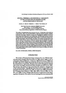
The Brazil-Malvinas confluence area (34°-46°S, 43°-60 W) is a highly dynamic region of the western boundary of the South Atlantic. A schematic representation of the geo­ strophic time averaged mass transport of the upper 1000 m based on the hydrographic data collected within the Conflu­ ence Program is shown in Figure 1 [Confluence Principal Investigators, 1990]. Two major CUITents with strongly con­ trasting water types, the Brazil and Malvinas (Falkland) currents, meet in this zone, generating a strong frontal structure and a complex aITay of eddies, rings and filaments [Gordon, 1989]. The contrasts in sea surface temperature (SST) and the local maximum in eddy kinetic energy make satellite infrared (IR) imagery [Legeckis and Gordon, 1982] and satellite altimetry [Provost et al., 1989] particularly appropriate tools to study the confluence region. The satel­ lite data provide valuable surface information in this remote area, which, like most of the southern hemisphere oceans, has few in situ time series observations . Most of our present knowledge of the variability in the confluence region cornes from previous studies using satel­ lite IR images which reveal several time and space scales of SST variability. Analyses of 3 years (July 1984 to June 1987) of satellite IR images have shown the dominance of an annual cycle [Podesta et al., 1991] and the existence of a Copyright 1993 by the American Geophysical Union. Paper number 93JCOO693. 0148-0227/93/93J C-00693$05 .00

semiannual signal [Provost et al., 1992] in the SST time variations. The location at which the Brazil CUITent separates from the coast appears to have annual and semiannual variations and seems to be situated further north during winter than during summer [OIson et al., 1988]. The associated fluctua­ tions of the western boundary of the warm water (Brazil CUITent) have meridional length scales of the order of 1000 km and zonal scales of 50 km [Legeckis and Gordon, 1982]. After separating from the western boundary, the Brazil CUITent joins with the return flow of the Malvinas CUITent and continues to flow in a general southward direction for sorne distance. The southern limit to the warm water bounded by the Brazil CUITent has been observed to fluctu­ ate between 38° and 46°S and 50° and 55°W, a distance of nearly 900 km, over time scales of about 2 months [Legeckis and Gordon, 1982]. The southward extensions of the Brazil CUITent are followed by the shed ding of warm-core eddies which are lost to the Subantarctic zone of the Antarctic Circumpolar CUITent. Those eddies formed during the north­ ward retreat of the Brazil Current are numerous and have a diameter of about 150 km [OIson et al. , 1988; Gordon, 1989]. After reaching a southern limit, the Brazil CUITent re­ verses direction and flows equatorward just east of its poleward flow. The western and eastern SST boundaries of the warm water overshoot are separated by 150 to 300 km [Legeckis and Gordon, 1982]. ConcuITently with the large-scale meridional frontal dis­ placements, time-dependent wavelike disturbances with

18,037

18,038

PROVOST AND LE TRAON: VARIABILITY IN BRAZIL-MALVINAS CONFLUENCE REGION

70'W

40'W 50' "'1IIIr.I'=~:-r-'-.--'-Y-",., 30'S

65'

35'

35'

40'

4S'

45'

50'S 70'W

65°

55'

50'

45'

Sehematic of geostrophic time averaged mass transport in the 1000 m in the western Argentine Basin hydrographie data eolleeted dudng the Confluence transports given are in sverdrups (1 Sv s -1) (Redrawn from Confluence Principal ln vestiga tors Figure 1].

scales occur intermittently. disof the western SST boundary associated with the Brazil CUITent can occur on time scales of about 1 week or longer, with along-stream scales of 200 km and Gordon, However the valuable information provided satellite IR should be examined carefully. Superficial ocean processes like the establishment of a shallow seasonal thermocline hide the "real" boundary between the Malvinas and Brazil currents characterized by the strong OIson et al" deeper front (Legeckis and Gordon, 1988]. This paper aims at describing the space and time sc ales of of the confluence using another type of altimetric data. Altimeter-derived sea level variations do not merely represent surface ocean !-,U''-'''VUl but rather show the dynamics of the whole water column. Data from altimetry a space-time coverage of the ocean that makes determination of mesoscale the For mesoscale space and characteristics time statistics in the North Atlantic have been derived in a manner from Geosat data Traon et al., 1990; Le Traon, 1991], and their significant differences in latitude and longitude have been related to different types of and dissipation mechanisms. The statistics of the whole southern ocean have been examined through satellite altimetric data Cheney 1985; Chelton et al., Chelton et al. [1990], 26 months of Geosat show that the strongest velocity variability in the first function (EOF) (which represents forced variability) occurs near the ,kt......."',,.,,1 front in each ocean basin. Otherwise, they find that mesoscale Îs strongest near the axis of the l-',u,'-"''',m.. UL~

Antarctic CUITent and suggest that il is related EOF to instabilities of the mean CUITent. In their analysis, 20 modes are needed to explain 80% of the vari­ ance. In each of the EOFs presented, the confluence appears as an extremum. They interpret the "white" char­ acter of the EOF spectrum as an indication that the coher· ence of the sea level variability in the southern ocean is fundamentally rather than zonal, even on the large space and time scales resolved by the smoothed data. In this paper the local sea lev el variability in the conflu­ is examined from a statistical point of view using ence sea 2 years of Geosat data. The method used for level residuals is described briefly. We discuss the issues of inhomogeneity and anisotropy in section 2. The aevellorlea in section 3 lead to a spectral characterization of the mesoscale and we address the issue of seasonal variability of the statistical and spectral character· istics. The Interpretation of the results follows in section 4 in relation to the characteristics of the atmospheric circulation. Section 5 summarizes the major results and provides the main conclusions. 2. INHOMOGENElTY AND ANISOTROPY We outline the data which is standard except for the orbit error removal (detailed in the appendix). Altimetric sea surface and abilities can provide useful information on and on spatial scales of variability. Anisotropy is then examined through the calculation of the main axes of vari· ance of velocity fluctuations.

Altimeter Data We used 2 years of Geosat data records (GDRs) obtained from the National Oceanic and Atmo­

2.1.

18,039

PROVOST AND LE TRAON: VARIABILITY IN BRAZIL-MALVINAS CONFLUENCE REGION

62'W

34'5

so'

S8'

SS'

S4'

52'

50'

48'

4S'

44'

1

1

___ 1 ______

42'W

3"·5

1

1

36'

3S'

38'

38'

40'

40'

42'

42'

...

44'

4S'S

82 e W

SO'

58'

S4'

S2'

50'

48'

...

Fig. 2. The study area in the South Atlantic (-45°-- 35°S, -65°_-45°W); the Geosat tracks are superimposed . The 23 tracks used in the analyses are labeled.

spheric Administration (NOAA) spanning the period from November 1986 to December 1988, i.e., 44 cycles of 17.05 days. The Geosat tracks over this region are shown in Figure 2. The average zonal distance between two adjacent tracks is about 1.4 degree of longitude. The distance between two data points on a track is 6.8 km. The procedures applied to process these data are described in detai! by Le Traon et al. [1990] and will be recalled only briefly here. The sea surface height (SSH) measurements were first cOITected for the following effects (corrections available in the GDRs): electromagnetic bias by adding 2% of significant wave height (H I13 ) to the SSH, ocean tides using the Schwiderski mode!, terrestrial tides using the Melchior model, ionospheric effects using the Global Positioning System climatic mode! , and dry and wet tropospheric effects using Fleet Numerical Oceanography Center data [Cheney et al., 1987]. Because of the uncertainties in estimating an inverted barometer correction [Zlotnicki et al., 1989], none was applied . The SSH profiles were then resampled regu­ larlyevery 10 km using a cubic spline (the initial sampling rate is 6.8 km) and the mean profile was subtracted from each individual profile. A polynomial adjustment with weights inversely propor­ tional to the mesoscale variance, thus taking into account the inhomogeneity of the mesoscale field (see appendix), was used to remove orbit error [Le Traon et al., 1991]. This gives the mesoscale sea level anomal y (SLA) sampled every JO km, at the time of the satellite pass on the given track. A Lanczos filter with a cutoff wavelength of 100 km was then applied to the SLA data to filter out instrumental noise . Geostrophic velocities were then obtained by centered finite differences. 2.2. Variability of Sea Level Anomaly and Surface Geostrophic Velocity Anomaly Maps of sea level anomaly variability have been obtained according to the method described by Le Traon et al. [1990] .

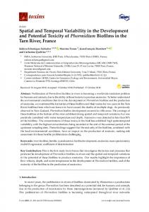
The study area is divided into 2° latitude by 2° longitude bins. Mean variances and associated errors are computed over each bin. Errors are assumed to have a Gaussian distribu­ tion, a decoITelation time of 34 days, and a spatial decorre­ lation scale of 100 km. These decorrelation scales corre­ spond roughly to the first zero crossing of spatial and temporal autocorrelation functions (see section 3). An ob­ jective analysis is then performed using Gaussian correlation functions with standard deviations of 2° in latitude and 2° in longitude . The associated error is generally of the order of 5% at 1 standard deviation. The region is very inhomogeneous: variabilities in SLA vary between 6 and 30 cm (Figure 3a). The maximum values are located from 39°S to 42°S in latitude and 54°W to 48°W in longitude and correspond to the frontal region separating the warm and salt y Brazil Current to the north from the cold and fresher Malvinas Current to the southwest [Leg eckis and Gordon , 1982]. The maximum variability does not occur at the separation of the currents from the coast but rather is sJightly offshore, over the 5000-m bathymetric isoline, i.e., on the offshore side of the continental slope. The variability also diminishes further offshore. Yariability is smaller in the Brazil CUITent (I6 to 12 cm) and even smaIJer in the Malvinas Current (below 8 cm). Eddies have been observed in the Brazil Current both by satellite data [Legeckis and Gordon, 1982] and with in situ observations [Evans and Signorini, 1985] . We have computed the corresponding surface geostrophic velocity anomalies (SG y A) assuming isotropic variability. The map of the SGYA variance (Figure 3b) shows values varying from 100 to 1700 cm 2 S-2. As is the case for the SLA, the maximum of variability is located between 39°S and 42°S and between 54°W and 48°W and is associated with the frontal region. However, in a frontal region such as the Brazil-Malvinas confluence, geostrophy may not be an ac­ curate approximation. The geostrophic variability obtained from altimetry compares well regarding both structures and

18,040

PROVOST AND

LE TRAON:

VARIABIUTY IN BRAZIL-MALVINAS CONFLUENCE REGION

-35

w

2 -40 ~

-45

a -65

. -60

-55

-50

-45

LONGITUDE

-35

show up here because of the particular orientation of ascend­ and arcs. To quantify anisotropy, we compute the principal axes of variance of velocity fluctuations. To do so, we need to estimate the components of the horizontal velocity correlation matrix. We first calculate the compo­ nents of the geostrophic velocity perpendicular to each track and at each crossover are then Iinearly to common and used to derive the zonal and meridional components u' and v' of the geostrophic fluctuations. Because of the orientation of the satellite tracks, the error on the geostrophic velocity estimates is anisotropie: the error on the meridional geo­ strophie velocity is about twice as as the one on the zonal velocity estimates. The covariances of fluctu­ ations, (U'2), (vil), and (u'v'), are then computed. The the principal axes of variance may be found by following problem et 1975]: .t\) - (U'v,)2 = 0

«U,2) - .t\)(v, 2)

The 0, the orientation of the principal axis measured counterclockwise from latitude is defined by

.......

w

2 -40

tan 20

3 -45 b -65

-60

-55 LONGITUDE

-50

-45

3. (a) Root square variability of sea level anomaly aCter wellZhtea polynomial adjustment (2-cm isolines4' Variance of the geostrophic velocity anomaJy (100 cm s isolines).

absolute values with the eddy kinetîc energy calcu­ lated from the drifting buoys of the First OARP Global [Patterson, 1985; Piola et al" 1987; and Van Loon, 1989; Johnson, 1989]. The 2° x 2° averaging and the objective analysis have reduced the observed maximum values. The variability obtained on the tracks can reach 40 cm for the SLA and 2500 cm 2 s for the EKE. However the statistical error on these point estimations along the tracks is high (above 15% and 30% at 1 standard deviation for SLA and EKE

= 2(u'v')/(u,2

The principal axes of variance 4a) show that the region is strongly anisotropic with meridional variances of velocity that are typically 3 times more important than zonal variances in the of maximum variability. Along the velo city fluctuations have a direction to the As the axes have preferentially a meridional direction, the anisotropy tends to ""'UU'.oal when on to the and descend­ ing arcs, and this is why maps obtained using only ascending arcs are similar to those obtained using only descending arcs. The main between those maps are indeed located in the where the principal axes do not have a meridional direction. The anisotropy ratio (greatest variance/smallest varies from 2 to 8 over the This ratio Fisher's law, and according to our decorrelation hypothesis (34 days, i.e., 1 cycle over 2), values greater than 2.5 are This anisotropy is maximum in the most em~rg(!tIc

-30

2000

cm'/s'

. 2,3.

,

-35

Anisotropy

The maps discussed above are obtained under the assump­ tion that variances along the and tracks are similar. A first way to characterize anisotropy for example, to calculate the variance of SOVA using only arcs (not shown) and only descending arcs (not shown), The statistîcal error on the se maps is typically greater than the error associated with 3a and 3b by a factor of 2 112 , and the differences between these maps are probably not Therefore the hypoth­ esis of isotropy those two directions happens to be rather weil verified in the confluence region. This does not mean, however, that mesoscale fluctuations are isotropie: for a zonal or meridional would not

v'2)

f '0 " .-ê

,

,

\

.. f " ~

\ \;

j.

t

. / f \ f " x " . ·11:";20 km d -) 0 and warm rings observed in satellite IR imagery [L and Gordon, 1982] certainly create sorne aliasing shorter periods onto longer periods. Two peaks at 50 da ys (values higher than 150 cm 2 ) ar 250 cm 2) is ot at periods between 75 and 150 days and wavelen about 500 km which tends to propagate westward: th maximum of energy is seen only on the spectra of p i tion toward the southwest and northwest (Figures 9c). The associated phase speeds of propagation va 6 to 4 cm s -1. The 80-day peak appears mostly propagation of direction southwest at a wavelength km . The 130-day peak appears for propagation botl southwest direction at a wavelength of 600 km an( northwest direction at a somewhat shorter wave I~ about 450 km. Third , there is a high peak at 500 km at a perio( days. This semiannual signal propagates essentially the north, with an important propagation to the n (Figure 9a) and a somewhat smaller propagation tOI northwest (Figure 9c). This semiannual signal is d and discussed further in section 4. There is no c1ear peak at the annual cycle in the a derived spectra. In the mean spectrum, the energ annual period is 3 times smaller than at the set period or at shorter periods (Figure 8). This is in with similar altimetry-derived spectra of the GuI region [Le Tmon, 1991], where the an nuai cycle de Except for the semiannual cycle and the peaks ( 70 days, most propagations are preferentially to' west. Very little energy is found in southeast pre direction . 3.5 . Seasonal Variations in the Spectral Characl In order to examine possible seasonal variations the sea level anomalies to compute the rms vari< austral summer (April 15 to October 15) (Figure 10 austral win ter (October 15 to April 15) (Figure 1

". "

35° S

....

I~O Pefi~obdO'f'l)

10ooPCllr~1obdOY'l)

10

la

1000 Porio1obdoys)

10

1000 Porio1obdoys)

10

V\t :::E"o. :::CJ'''' 10'[3"0. :::~ ,0;D 10(

:. '

. ... .. ' .

..

1000 Pcri'1obdoys )

40°

.'

la'

.~

2

45° S

\000

Pcrio10bdO~) la

:::lSJ'9OX 10

~

3

la' 5

0.001 0.0 10 O. \ 00 frequency (days~' 1

1000

0.001 0.010 0.100 freQuency (days")

la

:::5]''''''' 10 3

.

Pcrio~obdOY') la

la'

10'

la' 7

la' 10

0.001

0.010

0.100

0.001

fruquency (days-')

101,OO[J0 P'd010bdO~:o. la la·

Y\v

0.010

1000 PCrl°1obdOys)

la' 8

la' 11 0.001

1000 Pcrio10bdCYl)

1000 PcriofobdOYl)

1000 Pcrio1obooys)

la'

.10

la' 3

la' 6

la' 9

0.001 0.010 0.100 frequency (days~')

0.010

0.100

la

3

0.001 0.010 0.100 frequency (days"l

\000

Peri.

o

c ~ 10-1

'0

la l.g

CT V

(f)

n 0 z 'Tl

lO'~

1'°'

r

c ~ n

m

:;c m Cl

ô z C

la'

10­

10-' SPECTRUM

wovenumber NORTH-WEST PROPAGATION

9. smaller amount al 50 and the other al 130

10- 1

10-,1

d

10-'

10-'

10-' SPECTRUM

wovenumber SOUTH-EAST PROPAGATION

is observe
are one at 80

are observed al 130 and !iule e;nergy is observed in

10' 10- 1

18,045

PROVOST AND LE TRAON: VARIABILlTY IN BRAZIL-MALVINAS CONFLUENCE REGION

rately. The seasonal variations are still with respect to the mean over 2 years. Seasonal variations are small but signif­ icant (the error associated with one standard deviation is less than 10% on these maps). In summer the energetic central peak is intensified: the winter maximum is 28 cm, whereas the summer maximum reaches 32 cm and extends further south. However, the maxima remain at the same location. We also notice a summer intensification near the Rfo de La Plata estuary. The corresponding maps of isocorrelation at 17 days show that mesoscale structures are, in general, more correlated in summer. On the other hand, it seems that the southward extension of the central region in summer corresponds to structures poorly correlated in time (isocorrelation less than 15%). The comparison between wavenumber spectra in summer and in winter (not shown) shows that globally, the energetic level is higher in summer and that the difIerence occurs essentially at wavelengths larger than 300 km. Finally, we consider each year of data separately and recompute the variability statistics. The maximum in SLA rms variability reaches 32 cm the first year, whereas it is limited to 28 cm the second year. Although, the isocorrela­ tion at 17 days has values between 5 and 50% in each year, the spatial variation of the isocorrelation is quite difIerent and mesoscale structures are in general, more correlated the first year in the frontal region.

-35

4.

DISCUSSION

In this section we discuss the observed signais presented in section 3. We first focus on the signais with a period smaller than 150 days and then on the semiannual cycle. Finally, we discuss the total variability. 4.1.

Signais With a Period Less Than 150 Days

The signais with periods less than 150 days are of two types: highly energetic westward propagating signais respon­ sible for the peaks at 80 days and 130 days in Figures 8, 9b, and 9c, and the less energetic eastward propagating signais associated with the peaks at 50 and 70 days. For periods between 75 and 150 days, the signal shows a significant amplitude of around 15 cm only in the region where the water depth is deeper than 3000 m (figure not shown). In this band, most of the signal has a propagation direction to the west. The 80-day peak (propagation direction to the southwest at a wavelength of 500 km) may be related to the southward extension of the Brazil Current described by Legeckis and Gordon [1982). They report that the southern limit of this extension fluctuates within the region limited by the latitudes 38° and 46°S and longitudes 50° and 56°W, with time periods as short as 2 months. The 80-day peak described in section 3.5 corresponds fairly weil to those scales. One may wonder whether these westward propagating signals observed with Geosat are consistent with Rossby wave characteristics. In the presence of a mean zonal current U the dispersion relation for a first baroclinic Rossby wave is given by w = k(UK 2 - f3)/(K 2

-40

-45

a -65

-60

-55

-50

-45

LONGITUOE

-35

-40

-45 b

-65

"':60

-55

-50

-45

LONGITUDE

Fig. 10. Root-mean-square variability ofsea surface topography for (a) austral summer and (b) austral win ter (2 cm isolines). The energetic central part is intensified in summer and extends further to the south.

+ Ri- 2 )

where w is the angular frequency of the Rossby wave, K is its wavenumber (K 2 = k 2 + 12 ), k and 1 being the zonal and meridional wavenumber, respectively, f3 is the meridional variation of the Coriolis parameter, and Ri is the first internai Rossby radius of deformation. Given a mean Rossby radius of about 27 km for the region [Houry et al., 1987), a 500-km-wavelength Rossby wave with a northwest (south­ west) propagation should have a period of approximately 19 months in the absence of any zonal current (U = 0). A mean eastward zonal current U (U > 0, like the eastward CUITent of the Brazil-Malvinas confluence) would tend to increase further the period of the Rossby wave. Meridional variation ofbottom topography also modifies the dispersion relation of baroclinic Rossby waves. In the confluence region the ocean depth increases to the south by about 1 km over 1000 km, thus the topographie efIect is as important as the f3 efIect and will indu ce an even smaller phase velocity. Therefore the westward propagating signais observed in the average spec­ trum at periods from 75 to 150 days do not correspond to baroclinic Rossby wave characteristics. However, these signais do present characteristics that may be consistent with barotropic Rossby wave dynamics. In the absence of a mean current, a 5OO-km-wavelength barotropic Rossby wave with a northwest (southwest) propa­ gation should have a period ofapproximately 75 days. Both the eastward mean current (a few centimeters per second when averaged over the whole water column) and the meridional bottom slope (slight shoaling to the north with a slope of about 5 x 10 -4) will act to decrease the phase velocity and therefore increase the period. Therefore these westward propagating

18,046

PROVOST AND LE TRAON: V ARIABILITY IN BRAZIL-MALVINAS CONFLUENCE REGION

-35

w

g

-40

3

) -60

-65

-55 LONGITUDE

-50

-45

-35

..... W

'"::>

-40

3 -45 b -65

)MlI

.;

~

0

l'

ln

....,

5:0 Z

-se

-80

-!12

lonvltud•

-4a

-se

-80

-44

-!12

-4a

-se

-eo

-44

-!12

-4a

< :>

-44

longitude

LongIlude

'"~

r

=i

-


r r

j

i

~

fi),

!l

.~

.$

J!l

z

:>

V>

(') 0

Z

."

r

c: [Tl

z

() [Tl

?J

[Tl

-se

-tG

-20

-la

-la

Plate 1.

-!12 lOf\9''lude

-14

-'2

-4a

-la

-eo

-44

-a

-Ii

-se

-4

-2

-!12 lOf\9''lude

a

-4a

-eo

-44

-!12

-iii!

-4a

Cl

-44

Ô

longitude

2

6

a

la

12

'4

Z

15

Successive monthly maps of the semiannual signal over a full cycle (6 months). The semiannual signal appears as three large-scale

anomalies aligned parallel to the continental slope. These anomalies are ubiquitous in the frontal region.

18

20 00

o..,. -..J

18,048

PROVOST AND LE TRAON: VARIABILITY IN BRAZIL-MALVINAS CONFLUENCE REGION

b

case 1

·50

·45

·40

·36

-3D

·50

·45

-40

-35

-30

·36

-30

Lemude

LaUlude

clise l

·1i0

-4U

-40 I..IIUlude

·35

-30

·50

-45

·40 Lalllude

Fig. 12. Possible of the t:hree successive anomalies typical of the semiannual in term of variation in position of a with a recirculation cell on side. (a) Height profile h of a front with a recirculation cell on each side, taken the subtrack labeled 420 in Figure 2. (h) residual h' obtained by subtracting the mean (da shed Hne). 1 is a frontal excursion to the south; case a frontal excursion to the north.

This half yearly wave has becn observed in various fields in the atmosphere: in the temperature [Van Loon, 1967], in the 1972a; Hsu and Wallace, 1976], in pressure Van Loon, the wind (Van 1967, 1972b, Large and Van Loon, 1989] and in the [Van Loon, 1972c]. The semiannual wave is a marked feature of the southern hemi­ sphere circulation and dominates the of the annual curve of sea level pressure wind and temperature in the troiposplilel'e ...."!p'w,,,·rI of the subtropical A cornplete eX!)lallatllon this semiannual wave has not yet been [1967] relates it to the difference in and continental latitudes. The waves in pressure and zonal wind have aIl e!:ilJel:;lal.1)i at midlatitudes [Van Loon 1984a, b]. The semiannual wave in sea level pressure weil as the annual wave in wind or wind is second­ ary in the latitudes near 30"S over and where most of the variance is ex'plam(~d [Van 1972a, Van Loon and semiannual wave dominates over most of the middle and high southern latitudes. However, the semiannual wave in SLP at Port Stanley, Falkland Islands just 2° south of the studied here), represents only 30% of the total variance (probably due to the presence of the South American continent) whereas it explains over 70% in other middle-latitude open ocean locatîons of the southern hemi­ sphere [Van Loon and Rogers, 1984a]. Therefore according

to the literature, the semiannual wave should not be strong in the confluence and the hypothesis of a local wind forcing at the semiannual seems to be ruled out. The hypothesis of a remote influence with an mtlegr'ate:d effect of a wind at the semiannual is difficult to support, since the semiannual component appears to he weak in both the Malvinas and Brazil currents and to be strong only in the frontal region. At this stage, we have no of this semiannua! in the explanation as to the Brazil-Ma!vinas frontal system. 4.3.

The Full Mesoscale

The semiannual cycle, which is the most signal of the sea level variability as observed accounts for only 20% of the total variance. The full mesoscale i8 much more than the rather semiannual cycle described above. Sea surface topography anomal y maps have been com­ puted at intervals using optimal in space and time. The correlation functions have been deduced from the statistical of the previous section , e-folding distance of 100 km and e-folding time of 60 days). A series of 12 successive maps is shown in Plate 2, the first map to November 5, 1986. The anomaly values vary from -0.5 m (black areas, associated with relatively cold to 0.5 m (yeHow areas, warm In of the apparent complexity of the variability it is possible to identify severa! ocean processes occurring at

-40

{:

-+5r­

"0

:oc

0


OA

.~

(

1

t--

-65

-(5()

-00

-50

-45

••• ••

0.3 0.2 0.1 0.0 -0.1 -0.2 -0.3