Atmos. Chem. Phys., 14, 12085–12097, 2014 www.atmos-chem-phys.net/14/12085/2014/ doi:10.5194/acp-14-12085-2014 © Author(s) 2014. CC Attribution 3.0 License.
Spatial and temporal variability of sources of ambient fine particulate matter (PM2.5) in California S. Hasheminassab1 , N. Daher1 , A. Saffari1 , D. Wang1 , B. D. Ostro2 , and C. Sioutas1 1 University
of Southern California, Department of Civil and Environmental Engineering, Los Angeles, CA, USA Pollution Epidemiology Section, Office of Environmental Health Hazard Assessment, State of California, Oakland, CA, USA 2 Air
Correspondence to: C. Sioutas (
[email protected]) Received: 25 July 2014 – Published in Atmos. Chem. Phys. Discuss.: 4 August 2014 Revised: 2 October 2014 – Accepted: 4 October 2014 – Published: 18 November 2014
Abstract. To identify major sources of ambient fine particulate matter (PM2.5 , dp < 2.5 µm) and quantify their contributions in the state of California, a positive matrix factorization (PMF) receptor model was applied on Speciation Trends Network (STN) data, collected between 2002 and 2007 at eight distinct sampling locations, including El Cajon, Rubidoux, Los Angeles, Simi Valley, Bakersfield, Fresno, San Jose, and Sacramento. Between five to nine sources of fine PM were identified at each sampling site, several of which were common among multiple locations. Secondary aerosols, including secondary ammonium nitrate and ammonium sulfate, were the most abundant contributor to ambient PM2.5 mass at all sampling sites, except for San Jose, with an annual average cumulative contribution of 26 to 63 %, across the state. On an annual average basis, vehicular emissions (including both diesel and gasoline vehicles) were the largest primary source of fine PM at all sampling sites in southern California (17–18 % of total mass), whereas in Fresno and San Jose, biomass burning was the most dominant primary contributor to ambient PM2.5 (27 and 35 % of total mass, respectively), in general agreement with the results of previous source apportionment studies in California. In Bakersfield and Sacramento, vehicular emissions and biomass burning displayed relatively equal annual contributions to ambient PM2.5 mass (12 and 25 %, respectively). Other commonly identified sources at all sites included aged and fresh sea salt and soil, which contributed to 0.5–13 %, 2–27 %, and 1–19 % of the total mass, respectively, across all sites and seasons. In addition, a few minor sources were identified exclusively at some of the sites (e.g., chlorine sources, sulfate-bearing road dust, and different types of industrial emissions). These
sources overall accounted for a small fraction of the total PM mass across the sampling locations (1 to 15 %, on an annual average basis).
1
Introduction
Exposure to ambient airborne particulate matter (PM) is one of the leading causes of morbidity and mortality, contributing to more than 3 million premature deaths in the world annually, based on a recent global burden of disease study (Lim et al., 2013). PM inhalation has been linked to a wide range of adverse health effects such as respiratory inflammation (Araujo et al., 2008), cardiovascular diseases (Delfino et al., 2005; Ostro et al., 2014), and most recently neurodegenerative and neurodevelopmental disorders (Davis et al., 2013b, 2013a). For the past few decades, California has been constantly suffering from high concentrations of ambient PM, among the highest levels recorded within the United States, with estimated rates of PM-related morbidity and mortality exceeding any other state in the country (Fann et al., 2012). Ambient PM in California originates from a large number of diverse sources (Hu et al., 2014) and is a complex mixture of different chemical components, the composition of which may change drastically with PM size (Hu et al., 2008), location, and season (Cheung et al., 2011; Daher et al., 2013). Current PM regulations in California target PM10 and PM2.5 (particles with aerodynamic diameter less than 10 and 2.5 µm, respectively) mass concentrations, with PM2.5 being of major concern due to the higher rate of PM2.5 -related morbidity and mortality in the state compared to PM10 (Ostro
Published by Copernicus Publications on behalf of the European Geosciences Union.
12086
S. Hasheminassab et al.: Variability of sources of ambient fine particulate matter
et al., 2006; Woodruff et al., 2006). These regulations only target PM mass concentration, regardless of their sources of emission and/or toxico-chemical characteristics. There is, however, strong evidence that the level of toxicity and healthrelated characteristics of PM are significantly affected by their chemical composition and therefore by their emission sources (Rohr and Wyzga, 2012; Stanek et al., 2011; Zhang et al., 2008; Saffari et al., 2013). Recently, there has been growing interest in using source apportionment data in epidemiological health studies (Sarnat et al., 2008; Özkaynak and Thurston, 1987; Laden et al., 2000; Mar et al., 2000; Ostro et al., 2011). These studies have provided significant evidence that exposure to PM from certain sources is linked to mortality. In a recent study in Barcelona, Ostro et al. (2011) found that exposure to several sources, including traffic emissions, sulfate from ship emissions and long-range transport, and construction dust, is statistically significantly associated with all-cause and cardiovascular mortality. Nonetheless, to draw firm conclusions and develop more effective control strategies for reducing population exposure to harmful sources of airborne PM, further epidemiological studies that use source apportionment data are warranted. To date, several source apportionment studies have been conducted in California, using source-oriented (Hu et al., 2014; Kleeman and Cass, 2001; Zhang et al., 2014; DeNero, 2012) and receptor models (Hasheminassab et al., 2013; Hwang and Hopke, 2006; Ham and Kleeman, 2011; Kim and Hopke, 2007; Kim et al., 2010; Schauer and Cass, 2000). Source-oriented models focus on the transport, dilution, and transformation of pollutants from the source of emission to the receptor site, thereby providing an overall estimation regarding the spatial distribution of source contributions. Receptor models, on the other hand, focus on the behavior of ambient environments at the point of impact (Hopke, 2003). Even though these studies have provided important insights into the characteristics of sources of ambient PM as well as their relative contributions, they have been mostly conducted in a limited number of sampling locations and/or within a relatively short period of time. As a result, spatial and temporal variability of the identified sources have not been extensively examined. For instance, Kim et al. (2010) analyzed the PM2.5 speciation data collected between 2003 and 2005 at two sampling sites in southern California (i.e., Los Angeles (LA) and Rubidoux) to identify and quantify major PM2.5 sources, by application of a positive matrix factorization (PMF) model. Using a similar source apportionment approach, Hwang and Hopke (2006) evaluated the sources of ambient PM2.5 at two sampling sites in San Jose using the Speciation Trends Network (STN) data collected between 2000 and 2005. In a more comprehensive study, Chen et al. (2007) applied several receptor models to the chemically speciated PM2.5 measurements collected for 1 year (between 2000 and 2001) at 23 sites, all located in California’s San Joaquin Valley (SJV), to estimate PM2.5 source contributions.
Atmos. Chem. Phys., 14, 12085–12097, 2014
In this study, PMF, one of the most widely used receptororiented source apportionment techniques (Paatero and Tapper, 1994), was employed in order to provide a detailed and long-term (from 2002 to 2007) quantification of the contributions of different emission sources to ambient PM2.5 mass concentration in California, at eight distinct locations spanning the southern, central, and northern regions of the state. The association between PM-related mortality and PM2.5 mass concentration as well as individual PM2.5 chemical components has been investigated in previous epidemiological studies in California (Ostro et al., 2006; Ostro et al., 2007). The results of this study will be used as input for future epidemiological studies conducted by the California Environmental Protection Agency (Cal EPA) in order to further expand the current epidemiological knowledge by establishing the relationship between PM-related adverse health effects and specific source contributions. These findings will be crucial in establishing targeted and cost-effective regulations on PM2.5 emissions in the state of California.
2 2.1
Methodology Sampling sites
Sampling was conducted at eight STN sampling sites, established by the United States Environmental Protection Agency (US EPA), located in distinctly different cities all over California including El Cajon, Rubidoux, Los Angeles, Simi Valley, Bakersfield, Fresno, San Jose, and Sacramento. The studied sampling sites comprise a mixture of urban and semirural communities, with El Cajon and Rubidoux located in semi-rural areas while the rest of sampling sites are situated in densely developed urban regions of the state. Supplement Fig. S1 shows the location of all sampling sites. The Sacramento sampling site is located next to a park in a residential area with commercial establishments and highdensity residential homes in the surrounding neighborhood. It is also about 3 km southeast of a major freeway (I-80). The sampling site in San Jose is located 46 km east of the Pacific Ocean and 14 km southeast of the San Francisco Bay. It is also surrounded by primary commercial facilities (Hwang and Hopke, 2006). The cities of Fresno and Bakersfield are located in California’s heavily SJV (Zhao et al., 2011). These two cities are relatively far from the Pacific Ocean and are mostly impacted by secondary aerosols formed by emissions from upwind areas (Ying and Kleeman, 2006). Moreover, this part of the state usually suffers from severe particulate pollution, especially during the colder seasons (Kleeman et al., 2009). The northern parts of the SJV are dominated by agricultural activities, while the southern regions are mostly impacted by oil production (Held et al., 2004). The sampling site in Bakersfield is located about 6.5 km southwest of downtown, in a residential neighborhood and 2 km away from the nearest freeway (State Route (SR) 99). www.atmos-chem-phys.net/14/12085/2014/
S. Hasheminassab et al.: Variability of sources of ambient fine particulate matter The sampling site in Fresno is about 5.5 km northeast of the downtown commercial district (Watson et al., 2000), next to a four-lane artery with moderate traffic levels. Simi Valley is located 50 km northwest of downtown LA, in Ventura County, and the sampling site in this city is situated 500 m south of SR 118 (Kim and Hopke, 2007). Two sampling locations in the South Coast Air Basin were considered in this study; Los Angeles and Rubidoux. The sampling site in downtown LA is surrounded by three major freeways (i.e., I-110, I-5, and US-101) and is 30 km away from the ports of LA and Long Beach, both of which are among the busiest ports in the US (Minguillón et al., 2008). This sampling site is therefore heavily impacted by primary emissions. Rubidoux is situated 60 km inland from downtown LA and is typically subject to aged and photochemically processed particulate plumes advected from upwind regions (Sardar et al., 2005). Previous studies have reported high concentrations of ammonium nitrate in this region, which is mostly formed by the atmospheric reaction of nitric acid with ammonia from Chino dairy farms and livestock in upwind regions (Hughes et al., 1999). Lastly, the El Cajon sampling site is located in an inland valley, downwind of a heavily populated coastal zone, in San Diego County. This site is also impacted by emissions from the I-8 freeway, situated 500 m to its north. 2.2
Sampling schedule and chemical analysis
Time-integrated 24 h PM2.5 samples were collected between 2002 and 2007 at all sampling sites, except for LA and Rubidoux, where the STN data collected from 2002 to 2013 was used as the input file when running the PMF model (Hasheminassab et al., 2014). In the present study, in order to compare the results with those obtained for the rest of sampling sites, we calculated the average source contributions between 2002 and 2007 from the output of the same PMF runs which were originally conducted using the 2002– 2013 chemical data set. By performing a sensitivity analysis, Hasheminassab et al. (2014) showed that the results of the PMF model performed on the entire chemical data set (i.e., 2002–2013) is comparable to the output of the PMF model conducted separately on the 2002–2006 and 2008–2012 data sets in terms of the sources identified (similar number of sources with almost identical compositions) and the absolute source contributions (less than 18 % difference in average source contributions among all sources). The outcome of the sensitivity analysis thus indicated that the daily resolved source contributions between 2002 and 2007 are not significantly biased when the chemical data between 2008 and 2013 are also included into the PMF input file. During the studied period (i.e., 2002 to 2007), PM2.5 samples were collected every third day in Sacramento, San Jose, Fresno, Bakersfield, Rubidoux, and El Cajon sites, while every sixth day in Simi Valley and Los Angeles sites. Filter weighing and chemical analyses were performed according to the U.S. EPA Quality Assurance Project Plan www.atmos-chem-phys.net/14/12085/2014/
12087
(QAPP) (EPA-454/R-01-001) adopted for the STN field sampling. According to the QAPP, filters were tested, equilibrated, and weighted in the US EPA contract laboratories, and then they were shipped to the field. After sampling, filters bearing PM2.5 deposits were promptly shipped back to the laboratories for weight determination and other chemical analyses. PM2.5 mass concentration was determined gravimetrically by pre- and post-weighing the Teflon filters. Concentration of elements on Teflon filter samples was quantified by energy-dispersive X-ray fluorescence (ED-XRF) (RTI, 2009c). Major ions, including nitrate, sulfate, ammonium, sodium, and potassium, were measured by ion chromatography (IC) (RTI, 2009a, b). Elemental carbon (EC) and organic carbon (OC) were quantified from quartz filters, using the thermal/optical transmittance (TOT) NIOSH 5040 carbon method (Birch and Cary, 1996). 2.3
Source apportionment
In this study, the EPA PMF receptor model (version 3.0.2.2) was performed at each sampling site separately to identify the major sources of ambient PM2.5 and quantify their relative contributions to total PM2.5 mass. PMF is a factor analysis model that solves the chemical mass balance equations using a weighted least-squares algorithm and by imposing non-negativity constrains on the factors (Reff et al., 2007). 2.3.1
Data screening
The first step of data screening was correcting the OC data to account for sampling artifacts caused by adsorption and/or desorption of organic vapors on quartz filters (Chow et al., 2010). For each sampling site, the OC artifact was estimated using the intercept of the linear regression of OC against PM2.5 mass concentration (Kim et al., 2005). OC concentrations were then corrected by subtracting the OC artifact concentrations. The estimated OC artifact values (± standard errors) at each site are presented in Table S1. In addition, a detailed discussion on the year-to-year variability of the estimated OC artifacts is available in the Supplement. To avoid double counting of species, the linear correla+ + tions in each pair of S/SO2− 4 , Na/Na , and K/K were examined. Depending on the goodness of fit and the percent number of samples below detection limit (BDL) (threshold + + of 70 %), either IC SO2− 4 , Na , K or ED-XRF S, Na, K data were included in the PMF analyses. Measured BDL concentrations were replaced by half of the detection limit (DL) values, and their uncertainties were set as five-sixths of the DL values (Polissar et al., 1998). Missing values were replaced by the geometric mean of the existing concentrations, and their accompanying uncertainties were set as 4 times this geometric mean concentration. Species with more than 70 % BDL values as well as samples with missing mass and/or all of the elemental concentrations were excluded from the model. Lastly, occasional samples with unusually Atmos. Chem. Phys., 14, 12085–12097, 2014
12088
S. Hasheminassab et al.: Variability of sources of ambient fine particulate matter
high concentrations of a few chemical species, such as those collected around 4 July and/or New Year’s Eve with extremely high concentrations of K and/or K+ , were discarded. 2.3.2
PMF model
The uncertainties used in the PMF model were the estimated uncertainties reported in the Air Quality System (AQS) for the PM2.5 chemical speciation network. The uncertainties reported by STN include both the analytical uncertainties and uncertainties associated with the field sampling component (Flanagan et al., 2006). The uncertainties of elements, measured by the ED-XRF method, go through a comprehensive calculation procedure that harmonizes the uncertainties between different instruments and accounts for filter matrix effect, in addition to the field sampling and handling uncertainty (Gutknecht et al., 2010). For the other species, uncertainty is estimated as the analytical uncertainty of the instrument, augmented by 5 % of the calculated concentration, assuming that this 5 % is representing the total “field” variability (Flanagan et al., 2006). Species with a signal-to-noise (S / N) ratio between 0.2– 2, as well as those that have BDL values more than 50 % of total samples, were considered as weak variables and their uncertainties were increased by a factor of 3. In order to directly apportion the total PM mass, PM2.5 mass concentrations were included in the data matrix as a “total variable” in the PMF model (Lee et al., 2011). To ensure that the inclusion of total PM mass concentration does not affect the resulting PMF solution, their uncertainties were increased by a factor of 3, similarly to a weak variable (Reff et al., 2007). The model was performed in the default robust mode to diminish the influence of extreme values on the PMF solution, and the FPEAK parameter was applied to control rotational ambiguity (Paatero et al., 2002). Furthermore, a value of 5 % extra modeling uncertainty was applied. Uncertainties in the source profiles were estimated by a bootstrap procedure (Norris et al., 2008). Five hundred runs were considered for the bootstrap analysis in this study, and a solution was considered valid when the occurrence of unmapped factors was less than 10 % of the total runs. The final solutions were chosen based on the evaluation of the deduced source profiles and the quality of the chemical species fits by testing different numbers of factors.
3
Meteorology
Select meteorological parameters data, including temperature, relative humidity (RH), precipitation, as well as vectoraverage wind speed and direction were acquired from the online database of the California Air Resources Board (CARB). Table S2 presents the seasonal averages of these parameters at all studied sampling sites. In this study, seasons were defined as spring (March–May), summer (June–August), fall Atmos. Chem. Phys., 14, 12085–12097, 2014
(September–November), and winter (December–February), and seasonal/annual averages of all parameters reported in the following sections and shown in the figures and tables were calculated over all 6 years (i.e., 2002 to 2007). In addition, the standard errors accompanying the seasonal averages were calculated based on all daily resolved source contributions that fall within a given season. Details regarding the definition of standard error can be found in the Supplement. Lastly, in all of the figures and tables presented in this study, sampling sites were ranked according to their latitude, from south to north (i.e., from El Cajon to Sacramento). Most intense seasonality in temperature and RH was observed at the inland areas of the SJV, in Fresno and Bakersfield. These two sites experience the hottest and driest summertime weather across the state (temperatures over 25 ◦ C and RH below 45 %), while during winter, the mean temperature in these cities is within the lowest levels among all sites (below 10 ◦ C) and the RH reaches about 75 %, comparable to levels in other sites in the northern region of the state (i.e., San Jose and Sacramento). Unlike northern areas, in southern California RH exhibited more moderate seasonality, displaying minima in fall/winter (50–71 %) and maxima in spring/summer (59–77 %). At all sampling locations, the average of yearly total precipitation was negligible in summer but greatest in winter. During the studied period, Sacramento showed the highest total precipitation in winter, followed by LA, San Jose, and Simi Valley (23.4 ± 7.1, 21.7 ± 17.1, 16.3 ± 3.9, and 14.1 ± 13.0 cm, respectively). Additionally, wind speeds were generally much stronger in summer compared with fall/winter. During spring and summer, the wind blows mostly from the coast to inland in the southern part of the state (i.e., El Cajon, Rubidoux, LA, and Simi Valley), with a predominant westerly/southwesterly direction, while it shifts in winter and has a predominantly northerly origin at all sites with the exception of El Cajon. In Bakersfield and Fresno, the wind constantly blows from northwest throughout the year except for Fresno in winter, when wind has an easterly direction. Lastly, in Sacramento, the prevailing wind direction is southerly/southwesterly throughout the year.
4 4.1
Results and discussion Particulate mass
Seasonal average mass concentration of ambient PM2.5 at each sampling site is presented in Table 1. Overall, mass concentrations spanned a broad range of 8.2 to 36.6 µg m−3 across the studied sites and all seasons. PM2.5 mass concentration showed a very strong seasonality in central and northern parts of the state (i.e., Bakersfield, Fresno, San Jose, and Sacramento), with 2 to 4 times higher concentrations in winter compared with summer. This trend is typical of California’s Central Valley, which usually experiences the most severe winter particulate pollution in the US (Ying www.atmos-chem-phys.net/14/12085/2014/
S. Hasheminassab et al.: Variability of sources of ambient fine particulate matter
12089
Table 1. Seasonal average mass concentration (± standard error) (µg m−3 ) of ambient PM2.5 at the eight sampling sites in the period between 2002 and 2007.
Spring Summer Fall Winter
El Cajon
Rubidoux
Los Angeles
Simi Valley
Bakersfield
Fresno
San Jose
Sacramento
12.0 ± 0.5 13.1 ± 0.4 14.5 ± 0.5 17.1 ± 0.7
23.6 ± 1.3 25.6 ± 0.9 27.4 ± 1.5 20.0 ± 1.1
18.1 ± 1.5 20.2 ± 0.7 20.8 ± 1.2 20.4 ± 1.6
12.8 ± 0.8 15.9 ± 0.5 14.4 ± 0.9 9.8 ± 0.8
11.8 ± 0.5 13.5 ± 0.4 24.6 ± 1.7 32.0 ± 1.8
16.4 ± 1.1 9.7 ± 0.3 13.7 ± 0.6 36.6 ± 1.5
9.7 ± 0.4 9.6 ± 0.4 14.8 ± 0.8 18.6 ± 1.2
8.2 ± 0.3 9.2 ± 0.4 15.1 ± 0.9 23.5 ± 1.2
Table 2. Summary of the marker species for identified PM2.5 sources, resolved by the PMF model. Source
Marker species
Vehicular emissions Secondary ammonium nitrate Secondary ammonium sulfate Soil Fresh sea salt Aged sea salt Biomass burning Copper smelters Mixed industrial Chlorine sources Sulfate-bearing road dust Ni-related industrial sources
EC, OC, Fe, Cu, Zn, Pb, Mn + NO+ 3 , NH4 2− SO4 , NH+ 4 Al, Si, Ca, Fe, Ti Na+ , Cl− 2− Na+ , NO+ 3 , SO4 EC, OC, K/K+ Cu, EC EC, OC, Zn, Pb Cl− EC, OC, SO2− 4 ,Fe, Ca, Mn, Si, Ti Ni, Mn, Mg
and Kleeman, 2009). In winter, ambient PM2.5 mass concentrations peaked at Bakersfield and Fresno (32.0 ± 1.8 and 36.6 ± 1.5 µg m−3 , respectively). Severe stagnation periods and decreased mixing height are mostly responsible for elevated particulate pollution during winter in this part of the state. As it will be discussed in the following section, secondary ammonium nitrate and emissions from biomass burning were mainly responsible for elevated PM2.5 mass concentrations in these two cities during winter. In summer, on the other hand, the highest mass concentrations were observed in sampling sites located in the Los Angeles Basin (i.e., LA and Rubidoux). Rubidoux displayed the highest mass concentrations in fall, followed by summer and spring. In addition to local sources, this region of the state is typically subject to transported plumes from upwind regions in west and central LA (Daher et al., 2013; Sardar et al., 2005), particularly during the warm seasons when the westerly wind prevails (Table S2). 4.2 4.2.1
Source characterization and apportionment Overview
Between five to nine particle sources were identified at each sampling site. Resolved source profiles along with the explained variation (EV) of each species are shown in Fig. S2a– h for all studied sampling sites. Gray bars represent the normalized concentration of each species to the mass concentrawww.atmos-chem-phys.net/14/12085/2014/
Table 3. Summary statistics of the linear correlations between daily resolved measured ambient PM2.5 and estimated PM2.5 mass concentrations obtained from the PMF model. Errors correspond to 1 standard error.
El Cajon Rubidoux Los Angeles Simi Valley Bakersfield Fresno San Jose Sacramento
R2
Slope
Intercept (µg m−3 )
0.85 0.96 0.86 0.91 0.95 0.94 0.88 0.91
0.91 ± 0.02 0.91 ± 0.01 0.88 ± 0.02 0.91 ± 0.02 0.91 ± 0.01 0.91 ± 0.01 0.85 ± 0.01 0.83 ± 0.01
0.89 ± 0.26 1.30 ± 1.22 1.58 ± 0.47 0.84 ± 0.23 0.95 ± 0.24 1.01 ± 0.23 1.35 ± 0.23 1.47 ± 0.18
tion of PM2.5 apportioned to that factor, while the black dots represent the percent of each species apportioned to that factor (Lee et al., 1999). Table 2 summarizes the marker species which were used to identify each source profile. Several sources, including secondary ammonium nitrate, secondary ammonium sulfate, vehicular emissions, biomass burning, soil, and fresh and aged sea salt were commonly identified at multiple sites. A few minor sources were identified exclusively at some of the sites, depending on the site location and nearby emission sources. These sources, however, accounted for a small fraction of the total mass (1 to 15 % across the state, on an annual average basis). Table 3 presents the slope, intercept, and R 2 of the linear regressions between daily resolved measured ambient PM2.5 and estimated PM2.5 mass concentrations, calculated by the sum of PM mass apportioned to each identified factor. It can be inferred that the PMF model was able to effectively estimate the measured PM2.5 mass concentrations at all sites (slope varying from 0.83 to 0.91 and R 2 ranging from 0.85 to 0.96). Year-to-year variability in the source contributions was overall quite small for almost all identified sources. This can be deduced from the relatively small standard errors in the 6year seasonal average source contributions, as shown in Table S3a–d (median relative standard error of 8 %, across all sites, seasons, and sources). Identified sources, on the other hand, displayed distinct seasonal and spatial variability. The percent contributions from these sources to PM2.5 mass are Atmos. Chem. Phys., 14, 12085–12097, 2014
12090
S. Hasheminassab et al.: Variability of sources of ambient fine particulate matter
100%
Secondary nitrate Fresh sea salt Soil Other sources
7
a) Spring
100%
90%
90%
80%
80%
70%
70%
60%
60%
50%
50%
40%
40%
30%
30%
20%
20%
10%
10%
0%
0%
b) Summer
Vehicular emissions
6 Mass concentration (µg/m3)
Vehicular emissions Secondary sulfate Aged sea salt Biomass burning Unapportioned mass
5 4 Spring 3 2
Summer Fall winter
1 c) Fall
d) Winter
100%
100%
90%
90%
80%
80%
70%
70%
60%
60%
50%
50%
40%
40%
30%
30%
20%
20%
10%
10%
0%
0%
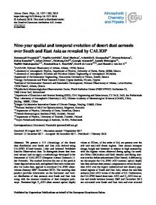
Figure 1 a-d. Seasonal variation in the percent contribution of identified sources to ambient PM , by site. Figure 1. Seasonal variation in the percent contribution of identified sources to ambient PM2.5 , by site (a–d). 2.5
32
presented in Fig. 1. Overall, secondary aerosols (including secondary ammonium nitrate and ammonium sulfate) collectively comprised the largest fraction of ambient PM2.5 at all sampling sites (except for San Jose), accounting for 26 to 63 % of total mass across all sites, on an annual average basis. Vehicular emissions were the second major contributor to PM2.5 at all sites (11 to 25 % annual average contribution, across the state), except for San Jose and Fresno, where biomass burning was the dominant primary source of PM2.5 (35 and 27 % annual average contribution, respectively). “Other sources” in Fig. 1 are associated with those sources which were identified exclusively at some specific locations. These contributed to < 15 % of the mass, on an annual average basis. The unapportioned mass, which is the difference between the seasonal average PM2.5 mass and the sum of the seasonal average source contributions from each factor, accounted for 3 to 6 % of total mass across the state, on an annual average basis. The unapportioned mass represents the fraction that could not be resolved by the model. 4.2.2
Vehicular emissions
Vehicular emissions source profiles were identified by high concentrations of carbonaceous species (i.e., EC and OC). Elevated loadings of several non-exhaust PM tracers (e.g., Fe, Cu, Zn, Pb, Mn) indicate that these sources are affected by particles emitted from brake and tire wear, road surface abrasion, and the resuspension of road surface dust (Pant and Harrison, 2013; Dall’sto et al., 2014). Only at Rubidoux was the PMF model able to determine two separate source profiles for diesel and gasoline vehicles (Fig. S2b). These source Atmos. Chem. Phys., 14, 12085–12097, 2014
0
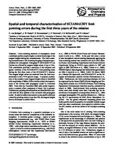
−3 ) oftovehicFigure 2. Seasonal average source contribution (µg/m3) of vehicular emissions ambient Figure 2. Seasonal average source contribution (µg m PM2.5, by site. Error bars correspond to one standard error.
ular emissions to ambient PM2.5 , by site. Error bars correspond to 1 standard error.
profiles are characterized by high loadings of EC and OC, respectively, with EC / OC ratios of 0.4 for the gasoline source profile and 2.2 for the diesel vehicles source profile. These ratios are within the ranges reported in previous studies (Liu et al., 2006; Fujita et al., 1998; Watson et al., 1998; Heo et al., 2009). Diesel vehicles operating at very low speed and in stop-and-go traffic usually produce similar EC / OC ratios to typical gasoline vehicles (Shah et al., 2004). As a result, the diesel emissions source profile that was obtained in Ru33 bidoux may represent only diesel vehicles driving in relatively constant speed in fluid traffic conditions, and the diesel emissions from stop-and-go traffic could be apportioned to the gasoline vehicles category. To overcome this uncertainty and also be able to compare the results with those obtained at other sampling sites, the contributions from diesel and gasoline vehicles were combined together at Rubidoux and referred to as vehicular emissions throughout the discussion. As can be seen in Fig. 2, across the state, estimated PM2.5 mass attributed to vehicular sources (including diesel and gasoline vehicles) reached their highest levels at Rubidoux, LA, and Sacramento, with annual average (± standard error) contributions of 4.3 ± 0.1, 3.6 ± 0.1, and 3.5 ± 0.1 µg m−3 , respectively. The spatial pattern of PM2.5 emissions from mobile sources across the state is in a good agreement with the findings of a recent study by Hu et al. (2014), in which they applied a source-oriented air quality model to predict primary PM2.5 source contributions across the state of California between 2000 and 2006. Vehicular emissions displayed similar seasonal patterns at all sampling sites, with higher contributions in fall and winter compared to spring and summer. In spring, summer, and fall, the highest vehicular emissions source contributions were observed at Rubidoux. In contrast, during winter, when particulate pollution is confined within the emission area due to higher atmospheric stability and lower mixing height, the www.atmos-chem-phys.net/14/12085/2014/
S. Hasheminassab et al.: Variability of sources of ambient fine particulate matter 20
Secondary nitrate
9
Secondary sulfate
8
16 14 12 Spring
10
Summer
8
Fall
6
winter
4
Mass concentration (µg/m3)
Mass concentration (µg/m3)
18
12091
7 6 5
Spring
4
Summer
3
Fall
2
winter
2
1
0
0
3 3 Figure 3. Seasonal average source contribution ) of secondary ammonium 4. Seasonal average source contribution ) of secondary Figure 3. Seasonal average source(µg/m contribution (µg m−3 ) ofnitrate sec-to Figure Figure 4. Seasonal average source(µg/m contribution (µgammonium m−3 ) ofsulfate sec-to ambient PM2.5 , by site. Errornitrate bars correspond to one standard error. ondary ammonium to ambient PM , by site. Error bars cor- ambient PM2.5, by site. Error bars correspond to one standard error.
2.5
respond to 1 standard error.
vehicular source contribution exhibited the highest value in downtown LA. This trend is typical of the LA Basin, in which downwind “receptor” areas are generally impacted by emissions from upwind “source” regions, when westerly/southwesterly onshore winds prevail (Table S2) (Daher et al., 2013). Several previous studies have reported similar trends in the LA Basin (Hasheminassab et al., 2013; Heo et al., 2013). It should be noted that after 2007 and until 2012, the contributions of vehicular emissions to ambient PM2.5 in the LA Basin statistically significantly decreased by 20 to 34 25 % following the implementation of major federal, state, and local regulations on vehicular emissions, particularly on diesel trucks (Hasheminassab et al., 2014). Among the studied locations in California’s Central Valley, vehicular emissions displayed the highest levels in Sacramento and lowest in San Jose, accounting for nearly 30 and 10 % of total mass, respectively, on average over 6 years. Vehicular emissions were comparable at Bakersfield and Fresno during spring and summer, whereas levels were slightly higher at Bakersfield in fall and winter. Schauer and Cass (2000) conducted a 4-day sampling in Bakersfield during the winter of 1995 to quantify the sources of ambient PM2.5 using chemical mass balance receptor model. The average wintertime level of vehicular emissions in our study at Bakersfield (3.0 ± 0.2 µg m−3 ) was about half of that reported by Schauer and Cass (2000) (6.3 ± 0.4 µg m−3 ), whereas the percent contributions of this source to total mass were comparable in both studies (10 and 12 %, respectively). This finding suggests that after almost a decade vehicular emissions have decreased by almost half in Bakersfield.
www.atmos-chem-phys.net/14/12085/2014/
ondary ammonium sulfate to ambient PM2.5 , by site. Error bars correspond to 1 standard error.
4.2.3
Secondary aerosols
Secondary ammonium nitrate source profile was identified + by high concentrations of NO− 3 and NH4 (Fig. S2a–h). Its contribution ranged from 0.2 to 16.8 µg m−3 , accounting for 3 to 55 % of ambient PM2.5 mass, among all sites and seasons, as displayed in Fig. 3 and tabulated in Table S3a– d. Seasonally, the contribution of secondary ammonium nitrate was largest in winter and lowest during summer, with statewide average contribution35 of 8.4 and 3.2 µg m−3 , respectively. Elevated concentration of secondary ammonium nitrate during the cold seasons is mainly due to the increased partitioning of ammonium nitrate into the particle phase, favored by lower wintertime temperatures and higher RH (Ying, 2011). This source displayed considerably higher contributions at Fresno and Bakersfield in winter (16.8 ± 1.3 and 15.8 ± 1.0 µg m−3 , respectively). Ying and Kleeman (2006) stated that diesel engines and catalyst equipped gasoline vehicles are important local sources that contribute to secondary nitrate in the SJV. Unlike all other sites, the seasonal trend of secondary ammonium nitrate was reversed at Rubidoux, with higher concentrations in summer compared to winter (12.5 ± 0.8 and 8.9 ± 0.8 µg m−3 , respectively). This is probably due to increased advection of ammonia from the upwind Chino area, caused by stronger westerly/southwesterly winds during summer in the LA Basin (Hasheminassab et al., 2013) combined with the increased photochemical production of nitric acid, which reacts with fugitive ammonia to produce high concentrations of ammonium nitrate in this area. The characterized secondary ammonium sulfate source + profiles have high loadings of SO2− 4 and NH4 (Fig. S2a– h). This source was identified at all sites, except at Fresno, where sulfate largely partitioned in a source named “sulfatebearing road dust” along with a few other components, which Atmos. Chem. Phys., 14, 12085–12097, 2014
12092 Biomass burning
10 8 Spring
6
Summer Fall
4
winter
2.5 2
Summer winter
0
0
biomass burning to ambient PM2.5 , by site. Error bars correspond to 1 standard error.
will be discussed in further detail below. Annual average contributions of this source ranged from 1.3 to 4.6 µg m−3 (or 10 to 24 % of total mass) among all sites, indicating that this source is a smaller contributor to total mass compared with secondary ammonium nitrate. Secondary ammonium sulfate exhibited a similar seasonal trend at all monitoring sites, displaying wintertime minima and peaks in summertime due to increased photochemical activity that forms this species. Levels were also overall higher in the southern part of the state compared to the upper regions (Fig. 4). As ar36 gued by Ying and Kleeman (2006), the majority of secondary aerosols formed in southern California are formed from locally emitted precursors, whereas in the SJV, secondary PM is mostly impacted by emissions from upwind areas (i.e., regional sources). Biomass burning
Identified biomass-burning source profiles consisted primarily of EC, OC, and either K or K+ (Fig. S2a–h). Biomass burning includes emissions from wildfires and residential wood combustion. This source showed distinct seasonal and spatial variability, with the highest levels observed during winter and also in upper parts of the state. Higher concentrations associated with biomass burning in winter are mainly due to higher residential wood burning during this season. Central and northern parts of the state usually experience colder winters compared to the southern regions (Table S2); therefore, higher biomass burning is expected in these geographical locations, as shown in many previous studies (Hu et al., 2014; Chen et al., 2007). Biomass burning was the major primary source of ambient PM2.5 at Fresno and San Jose during all seasons, with levels ranging from 2.4 to 10.4 µg m−3 (or 22 to 30 % of PM2.5 ) at Fresno and from 2.2 to 8.0 µg m−3 (or 22 to 43 % of PM2.5 ) in San Jose (Fig. 5). This source was also the dominant primary contributor to ambient PM2.5 Atmos. Chem. Phys., 14, 12085–12097, 2014
Fall
1 0.5
3 Figure 5. Seasonal average source contribution (µg/m ) of biomass burning to ambient Figure 5. Seasonal average source contribution (µg m−3 ) of PM2.5, by site. Error bars correspond to one standard error.
Spring
1.5
2
4.2.4
Soil
3
Mass concentration (µg/m3)
Mass concentration (µg/m3)
12
S. Hasheminassab et al.: Variability of sources of ambient fine particulate matter
Figure 6. Seasonal averageaverage source contribution (µg/m3) of soil(µg to ambient PMsoil 2.5, by Figure 6. Seasonal source contribution m−3 ) of tosite. Error bars correspond to one standard error.
ambient PM2.5 , by site. Error bars correspond to 1 standard error.
in Bakersfield and Sacramento during winter (12 and 31 % of PM2.5 , respectively), consistent with the findings of many previous studies in this area (Chow et al., 2007; Gorin et al., 2006; Schauer and Cass, 2000). 4.2.5
Soil
Resolved soil source profiles were dominated by crustal elements such as Al, Ca, Fe, Si, and Ti (Fig. S2a–h). These profiles generally lacked the contributions from EC and OC, indicating that they are not majorly impacted by emissions of road dust. As stated above, 37road dust was partially apportioned to the resolved vehicular emissions source profiles. A distinct source profile attributable to soil was not identified at Fresno. Instead, crustal elements partitioned in a separate source profile, along with high loadings of sulfate, EC, and OC, which was characterized as “sulfate-bearing road dust”. Across the state, soil exhibited lower concentrations in northern regions, namely at San Jose and Sacramento (Fig. 6). This is likely attributed to increased precipitation and higher RH in this part of the state (Table S2), which limit the windinduced resuspension of soil (Harrison et al., 2001). Soil, in contrast, accounted for a large fraction of PM2.5 at Bakersfield, in concert with the findings of Chen et al. (2007). During summer, in particular, the contribution of soil to total mass was near 20 % at Bakersfield, which could be mainly due to the lack of precipitation and low RH in this area (Table S2). As discussed by Chen et al. (2007), farm lands, pasture lands, and unpaved roads are major sources of soil and windblown dust in the SJV. 4.2.6
Fresh and aged sea salt
Sources with high concentrations of Na+ and Cl− were characterized as fresh sea salt (Fig. S2a–h). Aged sea salt source profiles, on the other hand, were dominated by loadings of − Na+ , SO2− 4 , and NO3 . Unlike fresh sea salt, chlorine has www.atmos-chem-phys.net/14/12085/2014/
S. Hasheminassab et al.: Variability of sources of ambient fine particulate matter Industrial emissions
0.8
3.5
0.6
0.4
Chlorine sources
3
*
**
Spring
* ***
Summer
Fall winter
0.2
Mass concentration (µg/m3)
Mass concentration (µg/m3)
1
12093
2.5 2 1.5 1
Spring Summer Fall Winter
0.5
0
0
3 FigureFigure 7. Seasonal source contribution (µg/mcontribution ) of industrial emissions to )ambient 7.average Seasonal average source (µg m−3 of indusPM2.5, by site. Error bars correspond to one standard error.
trial emissions to ambient PM2.5 , by site. Error bars correspond to 3 8. average Seasonal average (µg/m contribution (µgsources m−3 )toofambient chlorine FigureFigure 8. Seasonal contribution ) of chlorine PM2.5, by 1 standard error. site. Error bars correspond one2.5 standard error. sources to ambienttoPM , by site. Error bars correspond to 1 standard error.
a negligible or near-zero contribution to the aged sea salt source profile. Chlorine is typically depleted due to reactions of sea salt with acidic gases during the long-range transport of sea salt aerosols from the point of emission (Song and Carmichael, 1999). Aged sea salt overall accounted for a lager fraction (2 to 27 %) of ambient PM2.5 compared to fresh sea salt (1 to 13 %), in all sites and seasons (Figs. 1, S3, and S4). Aged sea salt showed a clear seasonal pattern at all sites, with higher concentrations in summer, consistent with increasing onshore winds (Table S1), and lowest during 38 winter. It is also noteworthy that the PMF model did not apportion a separate factor for ship emissions or a source related to ocean goods transport. However, high loadings of Ni and V (tracers of ship emissions (Arhami et al., 2009)) in secondary ammonium sulfate and aged sea salt source profiles for the sampling sites in the LA Basin, suggest that these sources are affected in part by emissions from ships serving the ports of LA and Long Beach (Hwang and Hopke, 2007). 4.2.7
Other sources
As noted above, a few sources were identified exclusively at some sites, with relatively low annual contributions to total mass (1 to 15 %, across the sites). At Rubidoux, a source profile was deduced with high loadings of Zn, Pb, EC, and OC (Fig. S2b), which is most likely attributed to local “mixed industrial” emissions in the surrounding areas. A similar source profile was also obtained in previous studies in this area (Kim and Hopke, 2007; Kim et al., 2010). At San Jose, a source profile dominated by Ni was identified, which likely indicates the contribution from nearby Ni-related industrial sources. Hwang and Hopke (2006) reported similar findings at the same sampling location by application of the PMF model on STN data, collected between 2002 and 2005. This source, nonetheless, accounted for less than 2 % of the total mass, on an annual average basis. The copper smelter source www.atmos-chem-phys.net/14/12085/2014/
profile, with a very high loading of Cu (> 80 %) and a slight contribution of EC, was identified in El Cajon and Bakersfield sampling sites (Fig. S2a, e). This source accounted for about 1 and 4 % of total mass, over all years, in Bakersfield and El Cajon, respectively. Figure 7 shows the seasonal trends of industrial emissions in locations where these sources were identified. In El Cajon and Rubidoux, the contributions of the identified industrial sources peaked in winter, while in Bakersfield and San Jose, maximum emissions from copper smelters and Ni-related sources were observed in summer. It is important to note that although the contributions from the identified industrial 39 sources to total PM mass were overall trivial (< 4 %), these sources and the related elements may be important contributors to the overall particle toxicity (Toledo et al., 2008; von Schneidemesser et al., 2010; Dall’osto et al., 2008; Saffari et al., 2013). At Fresno, a source profile with a high loading of sulfate along with road dust tracers, such as OC, EC, Fe, Ca, Mn, Si and Ti, was resolved (Fig. S2f). These road dust tracers most likely originate from the re-suspension of deposited soil and road dust enriched with vehicular emissions and lubricating oils (Pant and Harrison, 2013; Dall’sto et al., 2014). This source was therefore named “sulfate-bearing road dust” (Katrinak et al., 1995). As mentioned above, separate source profiles for secondary ammonium sulfate and soil were not identified at Fresno. Nonetheless, the relatively high loadings of sulfate and a few crustal elements (e.g., Al, Ca, Fe, and Si), along with the modest contribution of ammonium, suggest that these two sources are partially apportioned to this source profile. On an average basis over all 6 years, “sulfatebearing road dust” accounted for about 15 % of total mass at Fresno and its contribution was highest in summer among all seasons (2.7 ± 0.1 µg m−3 ). Atmos. Chem. Phys., 14, 12085–12097, 2014
12094
S. Hasheminassab et al.: Variability of sources of ambient fine particulate matter
Relatively similar source profiles, with high loadings of chlorine, were obtained at Fresno, Bakersfield, and Sacramento, with annual average contributions of about 5, 2, and 1 % to total mass, respectively (Fig. S2e, f, and h). This source, which was denoted as “chlorine sources”, was mostly detected during fall and winter at Fresno and Bakersfield, in the SJV, while it displayed the maximum seasonal average value in summer at Sacramento (Fig. 8).
Acknowledgements. This study was supported by the California Environmental Protection Agency (Cal EPA), Office of Environmental Health Hazard Assessment (OEHHA) (award no. 12-E0021). Edited by: A. Huffman
References 5
Summary and conclusions
Source apportionment analyses were conducted using a PMF receptor model applied on chemical speciation data sets, obtained from eight different STN sampling sites throughout the state of California, between 2002 and 2007. Five to nine major sources contributing to ambient PM2.5 were identified at each site, with several of which being common in multiple locations. Overall, secondary aerosols (including secondary ammonium nitrate and ammonium sulfate) were collectively the main contributor to PM2.5 mass at all sampling sites. Annual average source contributions of secondary ammonium nitrate and ammonium sulfate ranged from 3.1 to 12 µg m−3 (or 16 to 50 % of total mass) and 1.3 to 4.6 µg m−3 (or 10 to 23 % of total mass) across the state, respectively. On an annual average basis, vehicular emissions (including both diesel and gasoline vehicles) were the largest primary sources of PM2.5 at all sampling sites in the southern part of the state (i.e., El Cajon, Rubidoux, LA, and Simi Valley), with 17–18 % contribution total PM mass. In Fresno and San Jose, on the other hand, biomass burning was the dominant primary source of ambient PM2.5 , contributing to 27 and 35 % of total mass, on average over all years. In Bakersfield and Sacramento, vehicular emissions and biomass burning displayed relatively equal annual contributions to ambient PM2.5 mass (12 and 25 %, respectively). Other sources commonly identified at all sites were minor contributors to PM2.5 , including aged and fresh sea salt and soil, which contributed to 0.5–13 %, 2–27 %, and 1–19 % of total mass, respectively, across all sites and seasons. Furthermore, a few sources (including chlorine sources, sulfate-bearing road dust, and different types of industrial emissions), which overall accounted for a small fraction of total mass (1 to 15 %, on an annual average basis), were solely identified at some of the sites. The Supplement related to this article is available online at doi:10.5194/acp-14-12085-2014-supplement.
Atmos. Chem. Phys., 14, 12085–12097, 2014
Araujo, J. A., Barajas, B., Kleinman, M., Wang, X., Bennett, B. J., Gong, K. W., Navab, M., Harkema, J., Sioutas, C., Lusis, A. J., and Nel, A. E.: Ambient particulate pollutants in the ultrafine range promote early atherosclerosis and systemic oxidative stress, Circ. Res., 102, 589–596, 2008. Arhami, M., Sillanpää, M., Hu, S., Olson, M. R., Schauer, J. J., and Sioutas, C.: Size-segregated inorganic and organic components of PM in the communities of the Los Angeles Harbor, Aerosol Sci. Tech., 43, 145–160, 2009. Birch, M. E. and Cary, R. A.: Elemental Carbon-Based Method for Monitoring Occupational Exposures to Particulate Diesel Exhaust, Aerosol Sci. Technol., 25, 221–241, 1996. Chen, L. W. A., Watson, J. G., Chow, J. C., and Magliano, K. L.: Quantifying PM2. 5 source contributions for the San Joaquin Valley with multivariate receptor models, Environ. Sci. Technol., 41, 2818–2826, 2007. Cheung, K., Daher, N., Kam, W., Shafer, M. M., Ning, Z., Schauer, J. J., and Sioutas, C.: Spatial and temporal variation of chemical composition and mass closure of ambient coarse particulate matter (PM10−2.5 ) in the Los Angeles area, Atmos. Environ., 45, 2651–2662, 2011. Chow, J. C., Watson, J. G., Lowenthal, D. H., Chen, L. W. A., Zielinska, B., Mazzoleni, L. R., and Magliano, K. L.: Evaluation of organic markers for chemical mass balance source apportionment at the Fresno Supersite, Atmos. Chem. Phys., 7, 1741– 1754, doi:10.5194/acp-7-1741-2007, 2007. Chow, J. C., Watson, J. G., Chen, L.-W. A., Rice, J., and Frank, N. H.: Quantification of PM2.5 organic carbon sampling artifacts in US networks, Atmos. Chem. Phys., 10, 5223–5239, doi:10.5194/acp-10-5223-2010, 2010. Daher, N., Hasheminassab, S., Shafer, M. M., Schauer, J. J., and Sioutas, C.: Seasonal and spatial variability in chemical composition and mass closure of ambient ultrafine particles in the megacity of Los Angeles, Environmental Science: Processes & Impacts, 15, 283–295, 2013. Dall’osto, M., Booth, M. J., Smith, W., Fisher, R., and Harrison, R. M.: A study of the size distributions and the chemical characterization of airborne particles in the vicinity of a large integrated steelworks, Aerosol Sci. Tech., 42, 981–991, 2008. Dall’sto, M., Beddows, D. C. S., Gietl, J. K., Olatunbosun, O. A., Yang, X., and Harrison, R. M.: Characteristics of tyre dust in polluted air: studies by single particle mass spectrometry (ATOFMS), Atmos. Environ., 94, 224–230, 2014. Davis, D. A., Akopian, G., Walsh, J. P., Sioutas, C., Morgan, T. E., and Finch, C. E.: Urban air pollutants reduce synaptic function ˙ pathway in vitro, J. Neuof CA1 neurons via an NMDA/NO rochem., 127, 509–519, 2013a. Davis, D. A., Bortolato, M., Godar, S. C., Sander, T. K., Iwata, N., Pakbin, P., Shih, J. C., Berhane, K., McConnell, R., Sioutas, C.,
www.atmos-chem-phys.net/14/12085/2014/
S. Hasheminassab et al.: Variability of sources of ambient fine particulate matter Finch, C. E., and Morgan, T. E.: Prenatal exposure to urban air nanoparticles in mice causes altered neuronal differentiation and depression-like responses, PLoS ONE, 8, e64128, doi:10.1371/journal.pone.0064128, 2013b. Delfino, R. J., Sioutas, C., and Malik, S.: Potential role of ultrafine particles in associations between airborne particle mass and cardiovascular health, Environ. Health Persp., 113, 934–946, 2005. DeNero, S. P.: Development of a Source Oriented Version of the WRF-Chem Model and its Application to the California Regional PM10 /PM2.5 Air Quality Study, University of California, Davis, 2012. Fann, N., Lamson, A. D., Anenberg, S. C., Wesson, K., Risley, D., and Hubbell, B. J.: Estimating the national public health burden associated with exposure to ambient PM2.5 and ozone, Risk Anal., 32, 81–95, 2012. Flanagan, J. B., Jayanty, R. K. M., Rickman Jr, E. E., and Peterson, M. R.: PM2.5 Speciation Trends Network: Evaluation of Whole-System Uncertainties Using Data from Sites with Collocated Samplers, J. Air Waste Manage. Asso., 56, 492–499, 2006. Fujita, E. M., Watson, J. G., Chow, J. C., Robinson, N. F., Richards, L. W., and Kumar, N.: Northern Front Range Air Quality Study, Volume C: Source Apportionment and Simulation Methods and Evaluation, Prepared for Colorado State University, Cooperative Institute for Research in the Atmosphere, Ft. Collins, CO, Desert Research Institute, Reno, NV, 1998. Gorin, C. A., Collett, J. L., and Herckes, P.: Wood smoke contribution to winter aerosol in Fresno, CA, J. Air Waste Manage., 56, 1584–1590, 2006. Gutknecht, W., Flanagan, J., McWilliams, A., Jayanty, R. K. M., Kellogg, R., Rice, J., Duda, P., and Sarver, R. H.: Harmonization of Uncertainties of X-Ray Fluorescence Data for PM2.5 Air Filter Analysis, J. Air Waste Manage. Asso., 60, 184–194, 2010. Ham, W. A. and Kleeman, M. J.: Size-resolved source apportionment of carbonaceous particulate matter in urban and rural sites in central California, Atmos. Environ., 45, 3988–3995, 2011. Harrison, R. M., Yin, J., Mark, D., Stedman, J., Appleby, R. S., Booker, J., and Moorcroft, S.: Studies of the coarse particle (2.5– 10 µm) component in UK urban atmospheres, Atmos. Environ., 35, 3667–3679, 2001. Hasheminassab, S., Daher, N., Schauer, J. J., and Sioutas, C.: Source apportionment and organic compound characterization of ambient ultrafine particulate matter (PM) in the Los Angeles Basin, Atmos. Environ., 79, 529–539, 2013. Hasheminassab, S., Daher, N., Ostro, B. D., and Sioutas, C.: Longterm source apportionment of ambient fine particulate matter (PM2.5 ) in the Los Angeles Basin: a focus on emissions reduction from vehicular sources, Environ. Pollut., 193, 54–64, 2014. Held, T., Ying, Q., Kaduwela, A., and Kleeman, M.: Modeling particulate matter in the San Joaquin Valley with a source-oriented externally mixed three-dimensional photochemical grid model, Atmos. Environ., 38, 3689–3711, 2004. Heo, J., Dulger, M., Olson, M. R., McGinnis, J. E., Shelton, B. R., Matsunaga, A., Sioutas, C., and Schauer, J. J.: Source apportionments of PM2.5 organic carbon using molecular marker Positive Matrix Factorization and comparison of results from different receptor models, Atmos. Environ., 73, 51–61, 2013. Heo, J.-B., Hopke, P. K., and Yi, S.-M.: Source apportionment of PM2.5 in Seoul, Korea, Atmos. Chem. Phys., 9, 4957–4971, doi:10.5194/acp-9-4957-2009, 2009.
www.atmos-chem-phys.net/14/12085/2014/
12095
Hopke, P. K.: Recent developments in receptor modeling, J. Chemometr., 17, 255–265, 2003. Hu, J., Zhang, H., Chen, S., Ying, Q., Wiedinmyer, C., Vandenberghe, F., and Kleeman, M. J.: Identifying PM2.5 and PM0.1 sources for epidemiological studies in California, Environ. Sci. Technol., 48, 4980–4990, 2014. Hu, S., Polidori, A., Arhami, M., Shafer, M. M., Schauer, J. J., Cho, A., and Sioutas, C.: Redox activity and chemical speciation of size fractioned PM in the communities of the Los Angeles-Long Beach harbor, Atmos. Chem. Phys., 8, 6439– 6451, doi:10.5194/acp-8-6439-2008, 2008. Hughes, L. S., Allen, J. O., Kleeman, M. J., Johnson, R. J., Cass, G. R., Gross, D. S., Gard, E. E., GÃlli, M. E., Morrical, B. D., Fergenson, D. P., Dienes, T., Noble, C. A., Liu, D.-Y., Silva, P. J., and Prather, K. A.: Size and Composition Distribution of Atmospheric Particles in Southern California, Environ. Sci. Technol., 33, 3506–3515, 1999. Hughes, L. S., Allen, J. O., Salmon, L. G., Mayo, P. R., Johnson, R. J., and Cass, G. R.: Evolution of nitrogen species air pollutants along trajectories crossing the Los Angeles area, Environ. Sci. Technol., 36, 3928–3935, 2002. Hwang, I. and Hopke, P. K.: Comparison of source apportionments of fine particulate matter at two San Jose speciation trends network sites, Journal of the Air & Waste Management Association (1995), 56, 1287–1300, 2006. Hwang, I. and Hopke, P. K.: Estimation of source apportionment and potential source locations of PM2.5 at a west coastal IMPROVE site, Atmos. Environ., 41, 506–518, 2007. Katrinak, K. A., Anderson, J. R., and Buseck, P. R.: Individual particle types in the aerosol of Phoenix, Arizona, Environ. Sci. Technol., 29, 321–329, 1995. Kim, E. and Hopke, P. K.: Source characterization of ambient fine particles in the Los Angeles Basin, J. Environ. Eng. Sci., 6, 343– 353, 2007. Kim, E., Hopke, P. K., and Qin, Y.: Estimation of Organic Carbon Blank Values and Error Structures of the Speciation Trends Network Data for Source Apportionment, J. Air Waste Manage. Asso., 55, 1190–1199, 2005. Kim, E., Turkiewicz, K., Zulawnick, S. A., and Magliano, K. L.: Sources of fine particles in the South Coast area, California, Atmos. Environ., 44, 3095–3100, 2010. Kleeman, M. J. and Cass, G. R.: A 3-D Eulerian source-oriented model for an externally mixed aerosol, Environ. Sci. Technol., 35, 4834–4848, 2001. Kleeman, M. J., Riddle, S. G., Robert, M. A., Jakober, C. A., Fine, P. M., Hays, M. D., Schauer, J. J., and Hannigan, M. P.: Source Apportionment of Fine (PM1.8 ) and Ultrafine (PM0.1 ) Airborne Particulate Matter during a Severe Winter Pollution Episode, Environ. Sci. Technol., 43, 272–279, 2009. Laden, F., Neas, L. M., Dockery, D. W., and Schwartz, J.: Association of fine particulate matter from different sources with daily mortality in six U.S. cities, Environ. Health Persp., 108, 941– 947, 2000. Lee, E., Chan, C. K., and Paatero, P.: Application of positive matrix factorization in source apportionment of particulate pollutants in Hong Kong, Atmos. Environ., 33, 3201–3212, 1999. Lee, H. J., Gent, J. F., Leaderer, B. P., and Koutrakis, P.: Spatial and temporal variability of fine particle composition and source
Atmos. Chem. Phys., 14, 12085–12097, 2014
12096
S. Hasheminassab et al.: Variability of sources of ambient fine particulate matter
types in five cities of Connecticut and Massachusetts, Sci. Total Environ., 409, 2133–2142, 2011. Lim, S. S., Vos, T., Flaxman, A. D., Danaei, G., Shibuya, K., AdairRohani, H., AlMazroa, M. A., Amann, M., Anderson, H. R., Andrews, K. G., et al.: A comparative risk assessment of burden of disease and injury attributable to 67 risk factors and risk factor clusters in 21 regions, 1990–2010: a systematic analysis for the Global Burden of Disease Study 2010, Lancet, 380, 2224–2260, 2013. Liu, W., Wang, Y., Russell, A., and Edgerton, E. S.: Enhanced source identification of southeast aerosols using temperatureresolved carbon fractions and gas phase components, Atmos. Environ., 40, Supplement 2, 445–466, 2006. Mar, T. F., Norris, G. A., Koenig, J. Q., and Larson, T. V.: Associations between air pollution and mortality in Phoenix, 1995–1997, Environ. Health Persp., 108, 347–353, 2000. Minguillón, M. C., Arhami, M., Schauer, J. J., and Sioutas, C.: Seasonal and spatial variations of sources of fine and quasi-ultrafine particulate matter in neighborhoods near the Los Angeles-Long Beach harbor, Atmos. Environ., 42, 7317–7328, 2008. Norris, G. A., Vedantham, R., Wade, K., Brown, S., Prouty, J., and Foley, C.: EPA positive matrix factorization (PMF) 3.0 fundamentals & user guide. Prepared for the US Environmental Protection Agency, Washington, DC, by the National Exposure Research Laboratory, Research Triangle Park., 2008. Ostro, B., Broadwin, R., Green, S., Feng, W.-Y., and Lipsett, M.: Fine particulate air pollution and mortality in nine California counties: results from CALFINE, Environ. Health Persp., 114, 29–33, 2006. Ostro, B., Feng, W.-Y., Broadwin, R., Green, S., and Lipsett, M.: The effects of components of fine particulate air pollution on mortality in California: results from CALFINE, Environ. Health Persp., 115, 13–19, 2007. Ostro, B., Tobias, A., Querol, X., Alastuey, A., Amato, F., Pey, J., Pérez, N., and Sunyer, J.: The effects of particulate matter sources on daily mortality: a case-crossover study of Barcelona, Spain, Environ. Health Persp., 119, 1781–1787, 2011. Ostro, B., Malig, B., Broadwin, R., Basu, R., Gold, E. B., Bromberger, J. T., Derby, C., Feinstein, S., Greendale, G. A., Jackson, E. A., Kravitz, H. M., Matthews, K. A., Sternfeld, B., Tomey, K., Green, R. R., and Green, R.: Chronic PM2.5 exposure and inflammation: determining sensitive subgroups in mid-life women, Environ. Res., 132, 168–175, 2014. Özkaynak, H. and Thurston, G. D.: Associations between 1980 U.S. mortality rates and alternative measures of airborne particle concentration, Risk Anal., 7, 449–461, 1987. Paatero, P. and Tapper, U.: Positive matrix factorization: a nonnegative factor model with optimal utilization of error estimates of data values, Environmetrics, 5, 111–126, 1994. Paatero, P., Hopke, P. K., Song, X.-H., and Ramadan, Z.: Understanding and controlling rotations in factor analytic models, Chemometrics and Intelligent Laboratory Systems, 60, 253–264, 2002. Pant, P. and Harrison, R. M.: Estimation of the contribution of road traffic emissions to particulate matter concentrations from field measurements: a review, Atmos. Environ., 77, 78–97, 2013. Polissar, A. V., Hopke, P. K., Paatero, P., Malm, W. C., and Sisler, J. F.: Atmospheric aerosol over Alaska: 2. Elemental composition and sources, J. Geophys. Res. Atmos., 103, 19045–19057, 1998.
Atmos. Chem. Phys., 14, 12085–12097, 2014
Reff, A., Eberly, S. I., and Bhave, P. V.: Receptor modeling of ambient particulate matter data using positive matrix factorization: review of existing methods, J. Air Waste Manage., 57, 146–154, 2007. Rohr, A. C. and Wyzga, R. E.: Attributing health effects to individual particulate matter constituents, Atmos. Environ., 62, 130– 152, 2012. RTI: Standard Operating Procedure for the X-ray Fluorescence Analysis of Particulate Matter Deposits on Teflon Filters, Research Triangle Park, NC, 2009a. RTI: Standard Operating Procedure for PM2.5 Anion Analysis, Research Triangle Park, NC, 2009b. RTI: Standard Operating Procedure for PM2.5 Cation Analysis, Research Triangle Park, NC, 2009c. Saffari, A., Daher, N., Shafer, M. M., Schauer, J. J., and Sioutas, C.: Seasonal and spatial variation in reactive oxygen species activity of quasi-ultrafine particles (PM0.25 ) in the Los Angeles metropolitan area and its association with chemical composition, Atmos. Environ., 79, 566–575, 2013. Sardar, S. B., Fine, P. M., and Sioutas, C.: Seasonal and spatial variability of the size-resolved chemical composition of particulate matter (PM10 ) in the Los Angeles Basin, J. Geophys. Res.Atmos., 110, D07S08, doi:10.1029/2004JD004627, 2005. Sarnat, J. A., Marmur, A., Klein, M., Kim, E., Russell, A. G., Sarnat, S. E., Mulholland, J. A., Hopke, P. K., and Tolbert, P. E.: Fine particle sources and cardiorespiratory morbidity: an application of chemical mass balance and factor analytical source-apportionment methods, Environ. Health Persp., 116, doi:10.1289/ehp.10873, 2008. Schauer, J. J. and Cass, G. R.: Source apportionment of wintertime gas-phase and particle-phase air pollutants using organic compounds as tracers, Environ. Sci. Technol., 34, 1821–1832, 2000. Shah, S. D., Cocker, D. R., Miller, J. W., and Norbeck, J. M.: Emission rates of particulate matter and elemental and organic carbon from in-use diesel engines, Environ. Sci. Technol., 38, 2544– 2550, 2004. Song, C. H. and Carmichael, G. R.: The aging process of naturally emitted aerosol (sea-salt and mineral aerosol) during long range transport, Atmos. Environ., 33, 2203–2218, 1999. Stanek, L. W., Sacks, J. D., Dutton, S. J., and Dubois, J.-J. B.: Attributing health effects to apportioned components and sources of particulate matter: an evaluation of collective results, Atmos. Environ., 45, 5655–5663, 2011. Toledo, V. E., Júnior, P. B. d. A., Quiterio, S. L., Arbilla, G., Moreira, A., Escaleira, V., and Moreira, J. C.: Evaluation of levels, sources and distribution of toxic elements in PM10 in a suburban industrial region, Rio de Janeiro, Brazil, Environ. Monit. Assess., 139, 49–59, 2008. von Schneidemesser, E., Stone, E. A., Quraishi, T. A., Shafer, M. M., and Schauer, J. J.: Toxic metals in the atmosphere in Lahore, Pakistan, Sci. Total Environ., 408, 1640–1648, 2010. Watson, J. G., Fujita, E. M., Chow, J. C., Zielinska, B., Richards, L. W., Neff, W., and Dietrich, D.: Northern Front Range Air Quality Study, Final report, Prepared for Colorado State University, Cooperative Institute for Research in the Atmosphere, Fort Collins, CO, Desert Research Institute, Reno, NV, 1998. Watson, J. G., Chow, J. C., Bowen, J. L., Lowenthal, D. H., Hering, S., Ouchida, P., and Oslund, W.: Air quality measurements
www.atmos-chem-phys.net/14/12085/2014/
S. Hasheminassab et al.: Variability of sources of ambient fine particulate matter from the Fresno Supersite, J. Air Waste Manage., 50, 1321–1334, 2000. Woodruff, T. J., Parker, J. D., and Schoendorf, K. C.: Fine particulate matter (PM2.5 ) air pollution and selected causes of postneonatal infant mortality in California, Environ. Health Persp., 114, 786–790, 2006. Ying, Q.: Physical and chemical processes of wintertime secondary nitrate aerosol formation, Frontiers of Environmental Science & Engineering in China, 5, 348–361, 2011. Ying, Q. and Kleeman, M. J.: Source contributions to the regional distribution of secondary particulate matter in California, Atmos. Environ., 40, 736–752, 2006. Ying, Q. and Kleeman, M. J.: Regional contributions to airborne particulate matter in central California during a severe pollution episode, Atmos. Environ., 43, 1218–1228, 2009.
www.atmos-chem-phys.net/14/12085/2014/
12097
Zhang, H., DeNero, S. P., Joe, D. K., Lee, H.-H., Chen, S.-H., Michalakes, J., and Kleeman, M. J.: Development of a source oriented version of the WRF/Chem model and its application to the California regional PM10 / PM2.5 air quality study, Atmos. Chem. Phys., 14, 485–503, doi:10.5194/acp-14-485-2014, 2014. Zhang, Y., Schauer, J. J., Shafer, M. M., Hannigan, M. P., and Dutton, S. J.: Source apportionment of in vitro reactive oxygen species bioassay activity from atmospheric particulate matter, Environ. Sci. Technol., 42, 7502–7509, 2008. Zhao, Z., Chen, S.-H., Kleeman, M. J., Tyree, M., and Cayan, D.: The impact of climate change on air quality-related meteorological conditions in California. Part I: Present time simulation analysis, J. Climate, 24, 3344–3361, 2011.
Atmos. Chem. Phys., 14, 12085–12097, 2014