Spatial and temporal variation of bulk snow properties in northern

Geosci. Instrum. Method. Data Syst., 5, 347–363, 2016 www.geosci-instrum-method-data-syst.net/5/347/2016/ doi:10.5194/gi-5-347-2016 © Author(s) 2016. CC Attribution 3.0 License.

Spatial and temporal variation of bulk snow properties in northern boreal and tundra environments based on extensive field measurements Henna-Reetta Hannula1 , Juha Lemmetyinen1 , Anna Kontu1 , Chris Derksen2 , and Jouni Pulliainen1 1 Arctic

Research, Finnish Meteorological Institute, Sodankylä, 99600, Finland Research Division, Environment Canada, Toronto, Ontario, Canada

2 Climate

Correspondence to: Henna-Reetta Hannula ([email protected]) Received: 7 December 2015 – Published in Geosci. Instrum. Method. Data Syst. Discuss.: 18 January 2016 Revised: 8 June 2016 – Accepted: 25 June 2016 – Published: 8 August 2016

Abstract. An extensive in situ data set of snow depth, snow water equivalent (SWE), and snow density collected in support of the European Space Agency (ESA) SnowSAR-2 airborne campaigns in northern Finland during the winter of 2011–2012 is presented (ESA Earth Observation Campaigns data 2000–2016). The suitability of the in situ measurement protocol to provide an accurate reference for the simultaneous airborne SAR (synthetic aperture radar) data products over different land cover types was analysed in the context of spatial scale, sample spacing, and uncertainty. The analysis was executed by applying autocorrelation analysis and root mean square difference (RMSD) error estimations. The results showed overall higher variability for all the three bulk snow parameters over tundra, open bogs and lakes (due to wind processes); however, snow depth tended to vary over shorter distances in forests (due to snow–vegetation interactions). Sample spacing/sample size had a statistically significant effect on the mean snow depth over all land cover types. Analysis executed for 50, 100, and 200 m transects revealed that in most cases less than five samples were adequate to describe the snow depth mean with RMSD < 5 %, but for land cover with high overall variability an indication of increased sample size of 1.5–3 times larger was gained depending on the scale and the desired maximum RMSD. Errors for most of the land cover types reached ∼ 10 % if only three measurements were considered. The collected measurements, which are available via the ESA website upon registration, compose an exceptionally large manually collected snow data set in Scandinavian taiga and tundra environments. This information represents a valuable contribution to the snow research community and can be applied to various snow studies.

1

Introduction

A large set of in situ snow data were collected in support of European Space Agency (ESA) SnowSAR-2 airborne (Di Leo et al., 2015) acquisitions in northern Finland during the winter of 2011–2012 (Lemmetyinen et al., 2014). The airborne campaign was part of the feasibility study of the proposed ESA CoReH2O (Cold Regions Hydrology Highresolution Observatory; ESA, 2012; Rott et al., 2010) mission, at that time a candidate for the ESA Earth Explorer-7 satellite. The overall goal of the CoReH2O mission was to research the interactions between the cryosphere and climate. These included, but were not limited to, an estimation of the variation and amount of fresh water stored in snow cover, the links of the terrestrial cryosphere to the carbon cycle via soil freezing and respiration processes, and the role of snow cover in the global radiation balance (ESA, 2012). This paper addresses three subjects: (1) to describe an extensive data set of manual bulk measurements of snow acquired in northern Finland during the SnowSAR-2 campaign that is freely available for the snow research community, (2) to analyse and describe the spatial and temporal variability of these snow properties in different land cover types, and (3) to analyse the effect of scale and measurement spacing on the collected snow information as a ground-truth reference for airborne SAR (synthetic aperture radar) backscatter data. In the SnowSAR-2 campaign, the main focus was to test and develop an algorithm for snow water equivalent (SWE) retrieval, which is the product of snow depth (cm) and snow density (g cm−3 ) and quantifies the amount of water stored by the snowpack. For the campaign, a dual frequency (9.6

Published by Copernicus Publications on behalf of the European Geosciences Union.

348

H.-R. Hannula et al.: Spatial and temporal variation of bulk snow properties

and 17.2 GHz), two-polarization (VV and VH – vertical– vertical and vertical–horizontal) airborne SAR system (same measurement frequencies as the CoReH2O-satellite) was installed on a Piper PA-32 Saratoga aircraft. To better interpret the relationship between the snowpack properties and the SAR backscatter, ground measurements of snow depth and SWE were collected along the flight transects. As even in flat areas snow properties vary at a number of different scales (Derksen et al., 2010; Sturm and Benson, 2004), snow information retrieval via unmanned systems remains challenging. To develop a retrieval algorithm giving SWE values as close to reality as possible, it is important to analyse and quantify the spatial and temporal variability of SWE itself as well as snow depth and snow density. The SnowSAR-2 data were originally provided at 2 m or alternatively 10 m spatial resolution, but will be aggregated up to resolutions of 500 m. For this reason, it was important to assess the uncertainty in the in situ data itself, to evaluate the success of the measurement protocol (spacing and number of measurement points) to describe the apparent variation of the snow properties, and to estimate the variability of the measured snow data along scale changes. Numerous studies have described the spatial variability of snow properties in different environments. Many of them have concentrated on describing the statistical relationship between the snow parameters and the landscape characteristics, such as elevation, slope, azimuth, vegetation, and solar radiation (e.g. Blöschl and Kirnbauer, 1992; Hosang and Dettwiler, 1991; Trujillo et al., 2009; Watson et al., 2006; Zheng et al., 2016). Studies have also evaluated the effect of different sampling protocols (orientation, spacing, sample size etc.) on the measured (snow) information (e.g. Skøien and Blöschl, 2006; Trujillo and Lehning, 2015), and their ability to represent the “average” snow conditions (e.g. Chang et al., 2005; López-Moreno et al., 2011; Neumann et al., 2006). The proper sampling plan is especially essential for small sample sizes to minimize the uncertainty (McCreight et al., 2014). During recent years, studies utilizing airborne lidar (light detection and ranging) data (e.g. McCreight et al., 2014; Trujillo et al., 2007; Zheng et al., 2016) have offered new insight into these research questions as a considerable number of measurement points can been obtained in a short time from a relatively large areas. However, the temporal and spatial coverage of the snow measurements collected in the SnowSAR-2 campaign in northern boreal and tundra environments are still unique, and can thus be considered to offer unique information for scaling studies. Many of the previous collected data sets have been more limited either in time or space, or have been gathered in different land cover environments, for example, in an alpine environment, or by using e.g. lidar instruments. In this study, the analysis of the spatial heterogeneity of the snow properties and the effect of sampling spacing are specifically framed in the context of the ESA SnowSAR-2 airborne acquisitions, but the results can also be useful for planning future measurements in simGeosci. Instrum. Method. Data Syst., 5, 347–363, 2016

ilar environments, and further understanding of the nature of snow spatial heterogeneity. In the following sections, the key concepts to be used during the paper, such as scale, are discussed and defined. Then the collected data set and the methods to analyse the snow heterogeneity and the effect of sample spacing are introduced. Finally, discussion of the results in the context of the SnowSAR-2 campaign is given and the main findings are compared to previous studies.

2

Sampling procedure and scale

The difficulty to describe the spatial variability of snow properties is related to the fact that they are governed by different processes acting on different scales (Clark et al., 2011). For this reason, some understanding of this scale-dependent variation is necessary (Lloyd, 2014). Snow cover surface roughness that is affected by individual changes in vegetation or slope controls variance at very small scales. To estimate runoff at a watershed scale, coarser spatial information is adequate as this scale variability is mostly affected by, e.g., aspect, elevation, and land cover gradients (Clark et al., 2011). The dominant processes are not dependent only on scale, but also the type of environment (e.g. wind and topography in tundra landscape versus snow–vegetation interactions in the boreal forest) and they may work simultaneously at several scales (Blöschl, 1999). As such, the chosen measurement protocol can have a major effect on the results, and should be defined based on the local characteristics across the study domain, the purpose of the end user, and the amount of acceptable uncertainty. With point in situ sampling, the information gained will always, to some extent, be different from that of the actual snow patterns (Blöschl, 1999). The measurement error in the sampling itself, although not in the scope of this study, will add to uncertainty in the sample data. As such, analogously to previous studies, we will refer to the statistical characteristics of snow properties based on the SnowSAR-2 data set as apparent characteristics. The optimal sampling strategy would create a minimal bias (systematic error) and uncertainty (random error) (Skøien and Blöschl, 2006) between the variance of the sample data and the “true” pattern. The unrepresentativeness of point measurements for spatial means is well documented and usually increasing the number of samples decreases the uncertainty (e.g. Kuchment and Gelfan, 2001; Skøien and Blöschl, 2006; Yang and Woo, 1999). With intensive time demands when sampling in the field, knowledge of the most representative locations or the most optimal spacing of the measurement points is desirable. Blöschl and Sivapalan (1995) have introduced the term scale triplet to describe the three scales, which affect the measured sample data: spacing is the distance between measured samples, support quantifies the geometrical area/diameter of a single measurement point with a distinct method, and extent the overwww.geosci-instrum-method-data-syst.net/5/347/2016/

H.-R. Hannula et al.: Spatial and temporal variation of bulk snow properties all area covered by the measurements. Together this triplet forms the measurement scale or observation scale, which can be used to describe the spatial variation of a parameter. A process scale is the average distance over which a parameter varies in a landscape. We will utilize these defined concepts. In this study, the variation of bulk snow properties on scales from metres up to several hundred metres was the target of interest; to support the analysis of the SAR backscatter. For this purpose, an optimal sampling strategy would capture the “true” variation of SWE, snow depth, and snow density without significant under- or oversampling, at an accuracy superior to the one expected from the retrieved SnowSAR-2 geophysical data products (i.e. SWE). The analysis was executed separately for different land cover types. This was justifiable because processes affecting the spatial variation of snow depth and SWE are linked to the vegetation structure (or lack thereof). The review article of Varhola et al. (2010) drawing analysis upon 33 previous research articles from a time period spanning 1930s to 2010, showed that changes in forest cover explained 72 and 57 % of the relative changes in snow ablation and accumulation respectively. The sub-canopy snow depth is reduced as part of the precipitation is intercepted by the canopy and is sublimated or offloaded (e.g. Gelfan et al., 2004; Hedström and Pomeroy, 1998; Pomeroy et al., 1998; Storck et al., 2002). By reducing the passage of incoming solar radiation and by decreasing wind speeds, forest cover creates a sheltered environment slowing down the snowmelt and the sublimation loss from the ground (e.g. Gelfan et al., 2004; Hardy et al., 1997). In open areas, the snow cover is freely exposed to the atmosphere, increasing the sublimation loss, and creating a distinctly different energy balance from that of a forest (e.g. Harding and Pomeroy, 1996; Zhang et al., 2004). Forest edges and small openings may hold exceptionally deep snow depths depending on the wind speeds and the surrounding vegetation (Gary, 1975; Gelfan et al., 2004; Golding and Swanson, 1978; Veatch et al., 2009). The effect of vegetation structure especially applies to flat areas, such as the Sodankylä region, where elevation and aspect have little effect (D’Eon 2004). Remote sensing of snow cover has also proven to be problematic in the boreal forest zone (e.g. Foster et al., 2005; Heinilä et al., 2014) as the vegetation itself has a larger effect on the measurements and needs to be taken into account (Cohen et al., 2015; Derksen, 2008; Metsämäki et al., 2012). In tundra regions, local scale variability due to wind effects, and a stratigraphically complicated snowpack introduces different scales of variability (Derksen et al., 2010).

www.geosci-instrum-method-data-syst.net/5/347/2016/

349

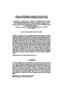
Figure 1. Snow depth (pink) and SWE (blue) measurements collected at the Sodankylä (left) and the Saariselkä (right) test sites during the SnowSAR-2 acquisitions.

3

Data and methods

3.1 3.1.1

Study sites Sodankylä

The in situ data used in this study were collected along the SnowSAR-2 flight lines over three sites during the winter of 2011–2012. One was located over sea ice in the Gulf of Bothnia, but these data are not covered here. Most acquisitions were located at the primary site, an approximately 7 by 10 km area close to the Arctic Research Centre of the Finnish Meteorological Institute (FMI-ARC) located near Sodankylä in northern Finland. The main site is a typical boreal forest/taiga environment dominated by spruce/scots pine forests of varying density, as well as open peatbogs (wetlands). The elevation in the area varies between 180 and 240 m above sea level and is relatively flat. The area covered by the SnowSAR-2 data also included several rivers and lakes. Acquisitions were timed to correspond closely to the planned CoReH2O revisit times during the two proposed phases of the mission (3- and 15-day revisit time). 3.1.2

Saariselkä

The second site was situated ∼ 150 km north of Sodankylä near Saariselkä, representative of an upland tundra environment. The area is mainly treeless, but the ground vegetation is characterized by lichen, mosses, and some larger shrubs, which result in a more variable local distribution of snow cover due to wind effects. The general topography was also more variable with several low-lying tundra hills situated along the acquisition path. This site was visited twice during the season; a single ∼ 20 km transect was covered. The aim was to provide data for CoReH2O retrieval performance testing over the tundra land cover type, which was not well represented at the main site.

Geosci. Instrum. Method. Data Syst., 5, 347–363, 2016

350

H.-R. Hannula et al.: Spatial and temporal variation of bulk snow properties

Table 1. Generalization of the field measurements based on the CLC2012 land cover classes analogous to Lemmetyinen et al. (2015), and the spatial %-coverage of each land cover group within a 7 km × 10 km area in the Sodankylä and the Saariselkä test sites. Acronym for generalized land cover group

3.1.3

Description

CLC2012 classes

DFm DFp SFm SFp FM

Dense forests (mineral soil type) Dense forests (organic/peat soil type) Sparse forests (mineral soil type) Sparse forests (organic/peat soil type) Fields and meadows

B OB LR O

Barren Open bogs Lakes and rivers Other (roads and urban areas)

Land cover

To study the spatial and temporal pattern of the snow properties in different land cover types, a land cover class for each snow measurement point was determined based on GPS coordinates, collected at each sample. The land cover information was available through the European Commission programme to COoRdinate INformation on the Environment (CORINE; http://land.copernicus.eu/pan-european/ corine-land-cover). A data set describing the land cover use and types during 2012 (CLC2012) was used. Analogous to former airborne data analysis from the site (Lemmetyinen et al., 2015) the original 44 CLC2012 land cover classes were generalized into nine land cover groups. Forested areas were divided based on both the total crown cover (> 30 % dense/ < 30 % sparse) and the soil type (mineral/peat or organic). The 30 % threshold value follows the classification of the CLC2012 data set where areas with a total crown cover exceeding 30 % and between 10 and 30 % are classified as dense forests and as sparse forests respectively. The division of forests on mineral and peat/organic soil was based on the hypothesized differences between these forest types; forests on peat/organic soil are former wetlands becoming forested and typically have lower canopy closure and tree height than the forests on mineral soil. Different types of open areas were also separated (wetlands/open bogs, meadows, barren surfaces, and water systems). The ninth group included all artificial surfaces, such as roads and buildings, and were excluded from the analysis. In Table 1, the nine generalized land cover groups, their acronyms used in this paper, and the spatial percent coverages of different land cover groups within a 7 km × 10 km area in the both test sites are shown.

Geosci. Instrum. Method. Data Syst., 5, 347–363, 2016

22, 24, 26, 27, 29 23, 25, 28 33, 35, 36 34 16, 17, 18, 19, 20, 21, 30, 31, 32 37, 38, 39 40, 41, 42, 44, 45 46, 47, (48) 1–15, 43

3.2 3.2.1

%-coverage on the 7 × 10 km area Sodankylä

Saariselkä

33 10 8 6 5

31 1 5 0 50

0 26 11 1

11 1 0 0

In situ measurements Snow depth

Ground sampling of the snow properties were made during the SnowSAR-2 flights. The main objective of the distributed measurements was to obtain a maximum amount of snow depth/SWE samples for comparison with the airborne observations. Around 600 SWE and 22 100 snow depth measurements were collected during a total of 19 days between December 2011 and March 2012. Table 2 represents the number of measurements within each land cover group per measurement day. The basic concept was to, at minimum, cover at least two 5 km transects for each flight. Sampling teams moved either on foot (snowshoes/skis), or by snowmobiles. At the main site, the sampling took place on most occasions during the day of the airborne acquisitions. On occasion, sampling was continued on the day following a flight, if the snow conditions remained stable. At Saariselkä, ground data were collected only on the dates of the airborne acquisitions. A total of 10 airborne acquisitions, as well as one dedicated calibration mission, were flown at the main site. Two acquisitions were flown at the Saariselkä tundra site. Snow depth was sampled every 100 m. At each measurement point, snow depth was recorded at minimum from three representative locations in a 10 m radius using a conventional snow probe (Fig. 1, left). An automated geolocated snow depth measuring tool (“Magnaprobe”, Snow-Hydro, Fairbanks, Alaska, USA) was also used on all sampling days (Fig. 1, middle). The Magnaprobe records the snow depth and the GPS position at the measurement point and stores the information in a data logger carried in a small backpack. For transects where the Magnaprobe was employed, snow depth was recorded considerably more frequently in distance (approximately every 2–10 m). Table 3 describes the approximate spacing, support and extent of the different measurement methods used during the campaign. www.geosci-instrum-method-data-syst.net/5/347/2016/

www.geosci-instrum-method-data-syst.net/5/347/2016/

LR

OB

B

FM

SFp

SFm

DFp

DFm

Land cover group

Dec 20

91 4 30 3 95 4 19 1 17 x x x 331 14 x x

x x x x x x x x 11 3 5 1 x x x x

Snow depth SWE

Dec 19

195 4 25 5 3 2 46 2 35 1 x x 333 25 42 1

Jan 9

x x x x x x x x x x x x 262 7 x x

Jan 10

172 7 24 2 74 4 17 2 37 2 2 x 123 23 375 10

Jan 23

218 8 72 4 81 2 38 2 7 2 x x 69 5 3 x

Jan 24

86 7 23 1 22 1 34 3 37 1 x x 281 11 32 2

Feb 7

20 6 23 2 45 2 11 1 28 4 2 x 55 5 254 10

Feb 8

17 3 5 2 13 4 3 x x x x x 45 9 1 1

Feb 9

587 13 193 4 241 6 141 4 138 10 x x 598 27 1098 8

Feb 22

1018 13 209 4 126 2 92 1 146 x x x 407 8 1 1

Feb 23

177 1 98 x 53 x 78 2 7 1 x x 791 8 x x

Feb 24

658 1 58 x 44 x 73 1 10 1 x x 2761 13 x x

Feb 25

116 12 55 2 32 4 63 5 45 1 x x 380 23 x x

Feb 26

11 x x x 16 x x x 3154 60 588 11 x x x x

Feb 29

1238 16 134 1 179 6 201 4 111 3 x x 1052 23 6 1

Mar 1

22 7 7 2 15 2 8 5 x x x x 60 9 4 1

Mar 5

58 6 41 1 36 4 53 3 x x x x 300 18 10 2

Mar 8

23 5 11 3 13 3 7 1 5 x x x 92 20 57 4

Mar 23

4887 113 1008 36 1120 46 884 37 3788 89 597 12 7940 248 1883 41

Total

Table 2. The in situ measurement dates and the number of snow depth and SWE/density measurements in the different land cover groups. Dates marked in bold indicate measurement days conducted at the Saariselkä test site.

H.-R. Hannula et al.: Spatial and temporal variation of bulk snow properties 351

Geosci. Instrum. Method. Data Syst., 5, 347–363, 2016

352

H.-R. Hannula et al.: Spatial and temporal variation of bulk snow properties

Table 3. Different measurement methods and their approximate spatial scales following the definitions of Blöschl and Sivapalan (1995). Spacing refers to the distance between the samples, support to the diameter of the individual sample, and extent to the overall areal coverage of the measurements. Method

Parameter

Spacing (m)

Support (cm)

Extent (km)

Snow probe Magnaprobe SWE coring tube

snow depth snow depth SWE (and density)

100 2–10 500

3 cm (3 samples) 2 cm 10 cm

7 × 10 7 × 10 7 × 10

Figure 2. Different methods utilized for snow depth and SWE measurements during the SnowSAR-2 campaign. Conventional snow probe (left), Magnaprobe (middle), and SWE coring tube (right).

3.2.2

Snow water equivalent

SWE was sampled every 500 m by using a SWE coring tube (Fig. 1, right). The tube was pushed through the snowpack, and snow depth was read from marks on the side of the coring tube. SWE (i.e. snow mass) was obtained by comparing the empty and full weight of the coring tube, while density was calculated based on the obtained SWE value and volume of the core sample (based on known radius of core and the measured snow height). The SWE measurement was taken from one representative location at each measurement point. 3.2.3

Snow density

SWE values for all the snow depth data points were determined to better allow for the analysis of the spatial variation of SWE. This was made based on the density information obtained from the distributed SWE measurements (every 500 m): ρb =

SWE . hb

(1)

Where ρ is the bulk (b) snow density and h is the total snow depth. Since fewer SWE than snow depth measurements were available, the density was determined per day per land cover group. If more than one SWE point was measured within the same land cover group during the same day, an average of these measurements was used. Sturm et al. (2010) Geosci. Instrum. Method. Data Syst., 5, 347–363, 2016

have shown that SWE distribution is mainly controlled by varying snow depth as snow density varies over a range much smaller than that of snow depth. However, the effect of this simplification was studied by comparing each measured density value to the average of other density values of the same land cover group on the same day when more than one measurement was available. The maximum and minimum differences in percentages (%) relative to the average value for each land cover group during the measurement campaign were recorded. In case no density information for a distinct land cover group was available, data from the previous or the subsequent measurement day was used, if no precipitation events or drastic temperature changes had occurred. On some occasions no applicable SWE measurement data were available; thus, for some snow depth data points no density and thus SWE information could be determined. The locations all of the collected ground measurements at the Sodankylä and the Saariselkä test sites are shown in Fig. 2. 3.3 3.3.1

Study methods Spatial and temporal variation of snow properties

The spatial and temporal variation of the bulk snow properties in different land cover groups was described and quantified. The three most important statistical characteristics to describe the variation of a parameter over a landscape are the integral scale (or autocorrelation), mean, and the variance (Skøien and Blöschl, 2006). The variation of snow depth, SWE, and snow density was described by constructing box plots of snow properties for each land cover group for each measurement day. To describe the overall average variation within each land cover group, the coefficients of variation (standard deviation divided by mean) were defined for each group for each measurement day. To easily compare the apparent spatial variability between the land cover groups, the values of coefficient of variation were averaged over the campaign period. The coefficient of variation was determined only for the snow depth data, as the comparatively low number of SWE/snow density measurements in different land cover groups during the campaign were not considered sufficient. The snow depth measurements, the most extensive part of the data set, allowed for further analysis of the apparent spatial variability of snow in different land cover groups. Most www.geosci-instrum-method-data-syst.net/5/347/2016/

H.-R. Hannula et al.: Spatial and temporal variation of bulk snow properties natural phenomena are, at least on some scale, spatially correlated (Atkinson and Tate, 2000). One of the basic principles of geostatistics is that observations near to each other are more likely to be alike than observations located farther apart. Spatial autocorrelation describes the spatial dimension over which a parameter varies (Blöschl, 1999), earlier defined as a process scale. This spatial dimension is described by a correlation length (Lex ), which is based on a semivariogram, in turn, characterising the average semivariance between two points (Skøien and Blöschl, 2006). A comprehensive description of a semivariogram and spatial correlation analysis can be found in the literature on geostatistics and spatiotemporal data (e.g. Christakos, 2000; Lloyd, 2014). For the autocorrelation analysis, snow depths measured with the Magnaprobe instrument were utilized, as these provided the necessary high spatial sampling spacing. In order to harmonize the analysis, multiple transects of 500 m were chosen from the collected data, representing each investigated land cover group. Autocorrelation was calculated as a function of lag distance. An exponential fit was applied to the autocorrelation, deriving the exponential (auto) correlation length (Lex ). The RMSD of the fit was also estimated. However, the data did not cover all land cover groups for all SnowSAR-2 acquisitions with a sufficient number of samples to conduct the autocorrelation analysis. The autocorrelation analysis was applied only for snow depths as SWE was estimated for each snow depth measurement point via land cover group fixed density and would have produced the same results. 3.3.2

Effect of sample size and spacing on the mean snow depth values

The effect of sample size and spacing on the mean snow depth values, typically used as a ground truth for airborne and space-borne data at various resolutions, was investigated by four different ways. Statistical similarity of the mean snow depths obtained via frequent and sparse measurements The difference between the mean snow depth values obtained from frequent Magnaprobe (potential over-sampling) measurements and the more sparse snow probe (potential undersampling) was statistically tested. Three land cover groups, DFm, OB, and LR, characterized by different average snow depths, and with sufficient Magnaprobe and conventional snow probe measurements were used for the comparison. The mean snow depth for both test groups of sample spacing for specific dates was calculated, and the difference of these values was statistically compared. No restriction for sample size was set; all qualified measurements were used leading into varying sample sizes. Statistical tests always lean on some assumptions, such as normality or equal variances, and to successfully use the test, www.geosci-instrum-method-data-syst.net/5/347/2016/

353

those assumptions should not be violated. Violation of normality assumption should not cause major errors if the sample sizes are > 30–40 (e.g. Ghasemi and Zahediasl, 2012). In our case the number of measurements within each sample varied. To be able to select an appropriate statistical analysis, each sub-group of the measurements was tested for normality and equality of variances. For some of the groups, the assumption of normality did not hold because snow depth distributions are limited by zero but essentially unbounded in the positive direction. As the assumption of equal variances also did not hold between all the compared groups, finally, both the Welsch’s unequal variances t test (assumes normality but not equal variances) as well as the Mann–Whitney U test (MWU) (assumes equal variances but not normality) were chosen for the statistical testing. The statistical methods used are widely described in the literature (e.g. Freund et al., 2010; Kanji, 2006). For each appropriate pair of snow depth test groups, the test statistic, p value, and the degrees of freedom were calculated. In statistical testing, the probability that the hypothesis set is true is tested. The null hypothesis (H0 ) set was there is no difference between the means of snow depth measured with frequent and sparse sample spacing. The alternative hypothesis (H1 ) was there is difference between the means, and the sample spacing has an effect on the measured mean snow depth value. The p value describes the probability that such a difference in mean snow depths that had been measured, or even higher than that, could be observed although the H0 was true; the smaller the p value the more likely the alternative hypothesis, H1 , was true. The p value was determined by calculating a test statistic from the sample measurements (t statistic / MWU statistic) and by comparing this test value to a threshold value of a chosen probability distribution (such as t distribution). The threshold value is dependent on the degrees of freedom (Df), describing the number of values in a sample that may vary independently, and the chosen significance level, which in this study was set to 0.05 or 5 %. If the p value was < = 0.05 the H0 was rejected and the probability the sampling spacing had an effect on the measured mean snow depth was deemed statistically significant. Effect of increasing measurement spacing on mean snow depth Further analysis of the Magnaprobe measurements was conducted to estimate the optimal sample spacing for each land cover type. For the analysis, further sub-transects of 50, 100, and 200 m were selected from the centre of each 500 m transect (used in the autocorrelation analysis), representing potential levels of aggregation of SnowSAR-2 data. For each of these sub-transects the “true” snow depth was calculated, assuming this to be the mean of all the Magnaprobe samples collected within the relevant transect. The mean snow depth of each transect was recalculated following an increasingly dense sample spacing, from three samples separated by Geosci. Instrum. Method. Data Syst., 5, 347–363, 2016

354

H.-R. Hannula et al.: Spatial and temporal variation of bulk snow properties

a maximum distance (Magnaprobe measurement at each end of transect + centre) up to using every second Magnaprobe measurement available. The resulting mean value was compared to the “true” snow depth, obtaining an RMSD versus increasing sample size (and decreasing sampling distance). The number of samples required to obtain an RMSD less than 5 % and less than 1 % was estimated from an exponential fit to the obtained RMSD vs. sample size. The RMSD of the fit in percentiles was also estimated. The same sub-transects were used to estimate the accuracy of the main snow depth sampling protocol (snow depth sampled by three samples every 100 m). The applied main sampling strategy was simulated by obtaining separately the mean of every adjacent three samples within the transect. This was compared to the “true” mean, obtaining an RMSD value. The mean of all calculated RMSDs was considered to represent the expected error of the sampling strategy (one set of three adjacent snow samples) against “true” average snow depth at 50, 100, and 200 m scales. Finally, it was studied if different measurement spacing leads to different outcomes when a weighted average of snow depth and SWE, based on land cover proportions within a typical remote sensing observation grid cell, were calculated; it was tested if the majority of the spatially distributed data, collected, e.g., at 100 m intervals, can provide an accurate reference, e.g., for the aggregated SnowSAR-2 products. For this purpose a 7 km × 10 km area was extracted from the CLC2012 land cover data and percent coverages of each generalized land cover group, both in the Sodankylä and in the Saariselkä test sites, were determined (Table 1). This area was approximately equivalent to the spatial extent of the ground measurements in the Sodankylä test site (Table 3). In the Saariselkä test site, the ground sampling occurred on a slightly smaller area; 4 campaign days with a high number of measurements were chosen for the analysis; 3 days from the Sodankylä test site and 1 day from the Saariselkä test site, as enough measurements were available from Saariselkä only from the second acquisition day. The distances between all the consequent measurements were calculated and three different cases of measurement spacing were compiled: one with maximum sample spacing (∼ every 1–10 m), one with medium sample spacing (∼ every 100 m), and one with sparse sample spacing (∼ every 500 m). However, as the measurement distances varied and were not always exactly every 100 m, it was not possible to produce withheld data with the exact sample spacing; for example, the 100 m case may actually vary between ∼ 70 and 150 m. However, the sample distances of the three cases were still clearly different. Proportionally weighted averages for both snow depth and SWE were calculated separately for each case of measurement spacing.

Geosci. Instrum. Method. Data Syst., 5, 347–363, 2016

4

Results

4.1

Land cover specific variation of snow properties

In the Figs. 3, 4, and 5 the box plots of snow depth, SWE, and snow density are presented. The red horizontal line marks the median, the blue box above and below the median mark the first quartile (Q1) and third quartile (Q3) respectively, representing the middle 50 % of the measurement values and as such also illustrate how variable the data are. The whiskers show the minimum and maximum values not considered as outliers (Q1 – inter-quartile range/Q3 + inter-quartile range), and black crosses note the outliers. In Fig. 4 the green median lines were added to mark the median derived only from the original SWE measurement values as the red median lines show the value derived from all the available SWE values including those calculated by utilizing the land cover group specific density information. The median snow depth of the LR was distinctly lower than those of the other land cover groups during the whole measurement campaign and varied approximately between 20 and 30 cm (Fig. 3). The snow depth in OB was typically several centimetres lower than in the forested land cover groups. This difference was more significant in the beginning and in the end of the measurement campaign than in the middle. This is in accordance with previous results from Neumann et al. (2006) and Goodison (1981), who noticed that there was a divergence of snow depth means between different types of sites as the snow season evolved. The median snow depth of the FM and the B were typically between those of forest cover groups and OB, being closer to the former. In the forested land cover groups, the median snow depth of the DFm was on average approximately 2–6 cm lower than the median snow depth of the DFp during most of the campaign period, but during some measurement days the relationship was the opposite. The highest variance in snow depth, according to minimum (2 cm) and maximum (120 cm) values was measured during the Saariselkä measurement day (29 February). For all other measurement days and land cover groups the highest median snow depths remained well below 80 cm. The SWE measurements in the different land cover groups (Fig. 4), show very similar results to snow depth, but the differences, for example, between the two dense and sparse forest groups were slightly clearer. For the calculated density, fewer measurements were available and on some days a single measurement might represent the snow density value in a land cover group (Fig. 5). The relationship between the density values of the land cover groups was different from those of snow depth and SWE, as densities were typically higher in the open areas than in the forested areas. The highest median density of 0.304 g cm−3 was measured in the LR on 9 January. The median density values measured in the FM and in the B in the Saariselkä test site on 29 February were also clearly more www.geosci-instrum-method-data-syst.net/5/347/2016/

H.-R. Hannula et al.: Spatial and temporal variation of bulk snow properties

355

Figure 3. Box plots of measured snow depth within each land cover group during the different field measurement days. Measurements from the Saariselkä test site are indicated in bold.

Figure 4. Box plots of measured SWE within each land cover group during the different field measurement days. Measurements from the Saariselkä test site are indicated in bold.

www.geosci-instrum-method-data-syst.net/5/347/2016/

Geosci. Instrum. Method. Data Syst., 5, 347–363, 2016

356

H.-R. Hannula et al.: Spatial and temporal variation of bulk snow properties

Figure 5. Box plots of measured snow density within each land cover group during the different field measurement days. Measurements from the Saariselkä test site are indicated in bold. Table 4. The minimum and maximum difference during the measurement campaign between a measured density value against an average of other density values representing n number of samples. The mean and standard deviation of exponential autocorrelation length (Lex ) of snow depth, and RMSD of the exponential fit over the land cover groups, calculated from representative transects during the snow sampling dates between 19 December 2011 and March 23, 2012. An averaged coefficient of variation for snow depth within each land cover group during the measurement campaign. The estimated RMSD of the nominal sampling protocol (as % of “true” snow depth), and the estimated number (threshold) of equally spaced samples required to achieve 5 and 1 % RMSD, for scales of 50, 100 and 200 m; an average of all acquisition dates by land cover types. Land over group

DFm DFp SFm SFp FM B OB LR

Difference in snow density (%)

Lex (m)

Snow depth (cm)

RMSD (%) for nominal protocol

No. of samples for RMSD < 5 %

No. of samples for RMSD < 1 %

min

n

max

n

mean

SD

exp fit RMSD

coefficient of variation

50

100

200

50

100

200

50

100

200

3.3 0.1 2.5 4 1.8 27.9 9.4 7.4

4 3 4 2 3 11 23 10

31.2 26.4 37.5 33.2 49.1 28.5 43.3 43.4

7 4 4 5 60 11 14 10

5.5 5.4 2.3 – 7.9 21.4 14.4 16.1

3.5 3.5 1.5 – 5.1 15.0 8.5 5.0

0.12 0.11 0.15 – 0.12 0.10 0.12 0.11

0.16 0.13 0.13 0.13 0.17 0.33 0.2 0.36

8.0 9.1 9.8 – 8.2 18.9 8.7 10.1

7.8 9.1 9.9 – 8.2 20.2 8.7 10.5

7.8 9.1 9.9 – 8.2 20.2 8.9 11.0

2.3 1.4 3.3 – 2.8 5.7 2.5 3.6

2.8 1.8 3.6 – 3.0 6.7 3.2 4.4

3.1 2.2 3.7 – 2.8 6.8 3.6 5.1

7.2 7.9 10.4 – 9.6 12.7 7.6 10.0

9.2 8.4 11.0 – 8.9 15.2 10.3 10.5

10.6 9.5 11.3 – 9.7 15.6 12.5 12.7

than 0.250 g cm−3 , as well as, the median densities measured in part of the forested groups towards the end of the campaign period. The highest variability in snow density was seen in measurements conducted on 29 February and in the OB during 19 December. The variability in the LR was very large; the density of this group was lower, and on some days much higher than in any other land cover group. It was also notable that the variation in density between the different land

Geosci. Instrum. Method. Data Syst., 5, 347–363, 2016

cover groups did not stay constant but as environmental factors changed, snow-bulk density in the different land cover groups reacted differently; on some days all the measured densities of the land cover groups were very close to each other, and on other days large differences existed. The maximum and minimum error the density simplification could introduce was estimated by comparison of each sample value with a sample mean. The analysis revealed few

www.geosci-instrum-method-data-syst.net/5/347/2016/

H.-R. Hannula et al.: Spatial and temporal variation of bulk snow properties very high densities which were potentially introduced by error in the sampling procedure. On 10 January one value of 0.619 g cm−3 had been measured in the LR with an average density within the group of 0.251 g cm−3 . This value was considered false and was removed from the analysis. Also on 19 December three high densities, 2–3 times higher than the average, one of them in the DFp and two in the OB, were measured, and were also left out when the final estimates of the density simplification error were calculated. The minimum/maximum difference (%) for all land cover groups representing (n) number of measurements during the measurement campaign are shown in Table 4. The maximum number of samples representing density within a land cover group during a single measurement day was 60, but in most cases this number varied between 2 to 30 (Table 2). An example of the autocorrelation of the measured snow depth over a representative transect is shown in Fig. 6 (top) for the OB land cover group. The correlation length (in metres) derived from an exponential fit is also displayed, providing a measure of the degree of variability in snow depth over distance. The mean and standard deviation of Lex and the RMSD of the fit (%), derived for the different land cover groups, is summarized in Table 4. The B land cover type represents data collected from the second Saariselkä campaign (average and standard deviation of Lex from 21 transects). On average, the DFm exhibited a low correlation length in snow depth, while values collected over the LR and the OB exhibited correlation lengths in excess of 14 m. Over the B landscape in Saariselkä, the average autocorrelation was in excess of 20 m. The RMSD of the fit in percentiles remained below 0.15 for all land cover groups. When the average of coefficient of variation for each land cover group, representing the whole campaign period, was calculated (Table 4), the dispersion of snow depth was highest over the LR and the B and remained low in the forested land cover groups and over the FM. Coefficient of variation for the same order of magnitude (from 0.12 to 0.22) for different types of sites in a boreal landscape, have been reported by Neumann et al. (2006) and for forested test sites by López-Moreno et al. (2011). 4.2

Effect of sample size, spacing, and the measurement protocol

The results from the statistical analysis of the difference of means in snow depth measured either every 2–10 m by Magnaprobe or approximately every 100 m by the conventional snow probe, are represented in Table 5. Both of the statistical tests gave similar results and clearly indicated an effect of sample spacing on the measured mean snow depth (rejecting the H0 ). Only on 26 February in the DFm did Welch’s test estimate the difference to be significant, whereas the MWU-test determined it insignificant. During most of the sample days, the difference between means was significant in the DFm and the difference remained rather constant, varying between approximately 3 and 6 cm, only increasing slightly towards the www.geosci-instrum-method-data-syst.net/5/347/2016/

357

Figure 6. Top: an example of an exponential fit to the calculated autocorrelation of snow depth measured over wetlands (OB) on 24 February 2012. Bottom: an example of mean RMSD against “true” snow depth with increasing sample size n for the same transect. Number of samples needed to achieve RMSD < 5 and < 1 % indicated.

end of the campaign. During 2 days with measurements from the LR, the difference in snow depth means was statistically significant. The observed maximum difference (cm) in mean snow depths on 23 January represented 18 and 15 % of the mean snow depth for Magnaprobe and conventional measurements respectively. The results from the comparisons in the OB were not consistent; during the first two sample days, the results were not statistically significant but during rest of the campaign, they were, with the difference between sample spacing protocols clearly increasing along the campaign period. The RMSD achieved using an emulation of the nominal sampling protocol of three adjacent snow depth samples is summarized in Table 4. The largest errors were apparent for the B land cover group (Saariselkä site), while the errors remained under 10 % for all other land cover groups except the LR. The lowest overall errors were estimated for the DFm. The investigated spatial scale affected results only marginally (less than 10 % for all land cover groups). Geosci. Instrum. Method. Data Syst., 5, 347–363, 2016

358

H.-R. Hannula et al.: Spatial and temporal variation of bulk snow properties

Table 5. The statistical difference of mean snow depth (cm) between the Magnaprobe and the sparse conventional measurements within DFm, OB, and LR. The number of measurements within a group (n), the mean snow depth, the difference in the mean measured snow depths, degrees of freedom (Df), test statistic (t/MWU), and the p value are presented. The p value is marked with ∗ if the result is statistically significant at 0.05. The test type considered more appropriate for each individual group, based on the distribution and variance of the data, is marked in bold. Date

Land cover class

magna 19 Dec 23 Jan 24 Jan 7 Feb 8 Feb 22 Feb 26 Feb

DFm OB DFm LR DFm OB DFm OB DFm LR DFm OB DFM OB

Mean (cm)

n

71 233 151 305 191 46 54 209 129 173 550 446 94 308

conv 20 98 21 70 27 23 32 72 71 81 37 152 22 72

magna 28.43 23.00 46.37 18.52 44.84 46.21 48.54 48.23 45.62 19.65 69.48 66.10 65.21 57.38

Difference (cm)

Welch’s t test

conv 32.30 22.99 50.30 21.72 47.97 41.70 53.84 45.22 51.64 22.14 70.71 57.38 69.44 50.86

Df 3.87 0.01 3.93 3.2 3.13 4.51 5.3 3.01 6.02 2.49 1.23 8.72 4.23 6.52

29.16 225.34 25.55 88.19 34.04 34.97 68.85 105.87 179.14 153.93 48.99 291.35 53.18 120.08

t statistic 2.596 −0.021 2.547 3.031 2.188 −2.068 3.730 −2.506 5.524 4.559 1.065 −8.591 2.284 −5.317

Mann–Whitney U

p 0.014∗ 0.983 0.017∗ 0.003∗ 0.036∗ 0.046 0.000∗ 0.014∗ 0.000∗ 0.000∗ 0.292 0.000∗ 0.026∗ 0.000∗

Df

MWU statistic

89 329 170 373 216 67 84 279 198 252 585 596 114 378

445.5 9993.0 1000.0 8224.0 1841.5 372.0 457.0 5563.0 2545.5 4561.0 9742.5 19 659.5 828.0 6883.0

p 0.011∗ 0.073 0.006∗ 0.003∗ 0.016∗ 0.046 0.000∗ 0.001∗ 0.000∗ 0.000∗ 0.665 0.000∗ 0.148 0.000∗

Table 6. The proportionally weighted averages of snow depth (cm) and SWE (mm) for the 7 km × 10 km land areas in the Sodankylä and the Saariselkä test sites (italic) for the three different cases of measurement spacing. Date 19 Dec 23 Jan 23 Feb 29 Feb

Snow depth Magnaprobe

100 m

500 m

SWE Magnaprobe

100 m

500 m

25.0 38.5 68.8 50.0

25.0 40.4 66.6 40.7

25.3 43.0 66.6 47.4

50.1 67.4 133.7 135.9

52.6 76.4 129.7 110.3

52.8 84.0 129.7 129.4

An average number of equally spaced samples required to reach a RMSD of less than 5 and 1 % of the “true” mean transect snow depth exhibited similar tendencies (Table 4). Fewer than five samples were required to characterize the mean snow depth with an RMSD lower than 5 % for most types of land cover at the investigated scales; an example is shown in Fig. 6 (bottom) for the OB land cover group on 24 February 2012. This would suggest a general sample spacing larger than that suggested by the Lex . An exception was the B land cover group at all three scales, represented by the Saariselkä tundra site. Results of the LR indicated an increase in required sample size, compared to other types of land cover at the Sodankylä site. Similar kind of results were shown by Neumann et al. (2006), who estimated the number of samples needed to represent a mean of 100 m snow depth transects at different sites. In their study, this amount varied between 1 and 44 but for most test sites during peak snow accumulation five samples represented the mean within 25 %. The number of samples required to characterize snow depth with an RMSD of less than 1 % was similarly the highest over the B land cover group, while in particular forested

Geosci. Instrum. Method. Data Syst., 5, 347–363, 2016

areas required the lowest number of samples. The number of samples required for both RMSD < 5 % and < 1 % typically increased with the investigated scale, with the exception of the FM, where the result was possibly affected by the low number of full 200 m transects sampled. For other types of land cover groups, increasing the investigated scale from 50 to 200 m increased the required number of samples from 10 to 45 %, or 9 to 63 % for errors of less than 5 % and less than 1 % respectively. The exponential fit used to calculate the 5 % and 1 % thresholds had, on average, an RMSD less than 0.9 percentiles in all cases. The weighted averages of snow depth and SWE based on land cover proportions in the 7 km × 10 km area are presented in Table 6. A consistent effect of the measurement spacing could not be determined; during the first 2 days investigated, the weighted averages increased slightly as the sampling spacing was decreased. During 23 February, the weighted average of snow depth and SWE showed very small decreases from 68.8 to 66.6 cm, and from 133.7 to 129.7 mm between the most frequent and the 100 m sampling case respectively. The 500 m sampling case did not introduce

www.geosci-instrum-method-data-syst.net/5/347/2016/

H.-R. Hannula et al.: Spatial and temporal variation of bulk snow properties change in these average values. At the Saariselkä test site, (29 February), the differences between the three cases were larger the average snow depth first decreasing ∼ 10 cm and then increasing ∼ 7 cm along the sparser sampling. Overall, the averaged SWE values changed more along with the sampling spacing than the values of snow depth. SWE estimated by using the land cover specific density values represent an additional source of error.

5

Discussion

The results of this study support the two previous general findings of open areas having more spatially heterogeneous snowpacks due to wind redistribution (e.g. Derksen et al., 2014; Essery and Pomeroy, 2004) than forested areas, whereas on the other hand, complicated canopy structure and small-scale ground topography affects the snow accumulation on the ground and increases the small-scale variability (e.g. Dobre et al., 2012; Storck et al., 2002); differences in snow depth and SWE variability (inter-quartile range in box plots in Figs. 3 and 4) between the land cover groups were often small, but the bulk snow properties measured at the Saariselkä test site, characterized by open tundra land cover type, had consistently higher deviation (inter-quartile range and minimum and maximum values) than the values at the mainly forested test site in Sodankylä. The mean values of coefficient of variation, showed the lowest variability in snow depth within the forested land cover groups (Table 4). However, the analysis of autocorrelation length (Lex ) presented in the Sect. 4.1 revealed that the snow properties tended to vary more on short distances in forests. This implies that although the absolute variation in snow depth was the largest in the sparsely vegetated areas, this heterogeneity appeared on scales larger than that in the forested groups. Earlier, Trujillo and Lehning (2015), Deems et al. (2006), and Trujillo et al. (2007) noted the different lengths of variability for snow depth over open and forested environments. Snow depth and SWE have similar spatial tendencies that are different than snow density due to the fact SWE is more dependent on snow depth than density as snow depth varies over a larger range (Sturm et al., 2010). For the same reason, smaller amount of snow density samples than snow depth samples have been considered to be adequate to estimate SWE over an area (e.g. Dickinson and Whitely, 1972). The analysis of frequently and sparsely (in distance) sampled snow depths indicated that different sample spacing protocols introduced a statistically significant difference in the mean snow depths within the tested land cover groups. Only in the OB the results were inconsistent perhaps because as the snow depth increases, wind redistribution increases the variability in the observed snow depth. In the LR the difference was significant during both days tested. This could be related to the overall high variation of snow depth on lakes and rivers (Table 4), which might be related to the fact that lakes www.geosci-instrum-method-data-syst.net/5/347/2016/

359

and rivers (including narrow creeks with typically deeper snow depths) were considered together. Although the differences were observed to be statistically significant, absolutely, they reached a maximum difference of approximately 8 cm against an average snow depth of 66.1/57.4 and 6 cm against an average snow depth of 45.6/51.6 cm for the OB and the DFm test groups respectively. This would have introduced a maximum “error” less than 15 %, and in most cases the error would have remained below 10 %. The success, however, of the sampling protocol is dependent on the desired scale to be quantified and the accepted amount of uncertainty. In the context of the SnowSAR-2 campaign, reasonably well representative results of mean snow depth characteristics, especially in the forested land cover groups, were achieved even with the protocol of sampling snow depth every 100 m. Watson et al. (2006) found that 65 % of the random SWE variability appeared at scales up to 10 m and 83 % at scales < 100 m. As such, the sampling protocol of this study can be considered to catch most of the snow depth variability to characterize the overall mean, but to determine, e.g., vegetation effects (Trujillo and Lehning, 2015), only the transects with Magnaprobe measurements would offer sufficiently intensive sample spacing. In an ideal situation, the sampling should be executed at least twice more frequently in distance than Lex so that the apparent variance at the considered scale could be captured. On the other hand, for the same reason sampled transects should represent lengths longer than Lex (López-Moreno et al., 2011). However, the RMSD analysis of the sample spacing (and thus the sample size) in transects of 200, 100, and 50 m, showed that in most of the land cover groups investigated, less than five samples were adequate to describe the average snow depth with a RMSD error less than 5 %. This, in turn, would generally mean spacing larger than that suggested by the autocorrelation, especially for the forested land cover groups. Even to gain RMSD error less than 1 %, the sampling spacing could generally be larger than that suggested by the Lex . If the desired result is to characterize the average snow depth (as it is for the aggregated SnowSAR-2 data products), sparser sampling protocol, than suggested by Lex , can be adequate in most of the land cover types represented in this study (also found by Trujillo et al., 2007). Over Barren lands (B) and in the LR, a higher number of samples was required and, as such, it might be reasonable to concentrate measurements in these land cover types. The autocorrelation analysis showed the small-scale snow depth variability in forests, and if the desired result is to characterize this instead of the mean pattern, sampling spacing suggested by the autocorrelation analysis would be more appropriate. The nominal process of snow depth measurements (three samples taken and averaged) introduced error less than 10 % in most of the land cover groups when compared to the “true” average snow depth of the transect. This kind of protocol may average out the measurement error and filter out very small-scale variability if it is not in the scope of the study Geosci. Instrum. Method. Data Syst., 5, 347–363, 2016

360

H.-R. Hannula et al.: Spatial and temporal variation of bulk snow properties

(Skøien and Blöschl, 2006). Averaging has a similar effect as has the increase of support; it decreases the overall statistical variability. This is why an increase in support, such as an increase of a footprint of a SAR product, decreases the amount of unresolved small-scale variability (Beckie, 1996). To characterize the mean snow depth within a passive microwave grid of 25 km × 25 km over the homogeneous Great Plains of the USA, “only” a minimum of 10 sample points was needed for error less than 5 cm (although error was dependent on snow depth) (Chang et al., 2005). In comparison, for a 10 m × 10 m plot with high snow depth variability, five samples would be needed to reduce the error of the mean estimate < 10 % (López-Moreno et al., 2011). However, it must be noted that the transects here represent rather short distances and the number of samples required for low RMSD error and the unrepresentativeness of a few point measurements naturally increases along the distance and the area to be characterized as well as along the complexity in terrain, vegetation variability, etc. (Yang and Woo, 1999). Different complexity along a different 100 m transect would produce different results. Because of the low overall variability in snow depth, few equally spaced samples were likely able to catch the variance with a reasonably low uncertainty in forests. In the B, the OB, and the LR more samples would be needed due to the high sub-interval variability between the samples (Trujillo and Lehning, 2015); with a small sample size, the measurements should also be located in the most optimal places to decrease uncertainty (McCreight et al., 2014). The effect of different sampling spacing on the spatially averaged snow depth and SWE values over the 7 km × 10 km areas was not clear (Table 6). The analysis gave some indication that the effect might be more significant in SWE than in snow depth measurements and that the effect increased as the snow depth increased along the snow season. Also Sturm et al. (2010), who used a statistical model to estimate snowbulk density based on the day of the year, climate class of snow, and snow depth, found that the probable error in SWE increased along with snow depth, but the relative error decreased along with increasing SWE. From the perspective of providing remotely sensed information for hydrology applications, the error during the peak accumulation is the most interesting as it defines the maximum amount of water to be released from the snowpack (Wetlaufer et al., 2016). The maximum difference the density simplification was estimated to introduce against the average value reached 49 % in the FM. Also in the OB and the LR the differences were clearly larger compared to other land cover groups. This is well in accordance with other results of the study as the highest error with such simplifications would occur in land cover groups with the highest spatial variability. A larger relative error would be introduced for shallow snow depths (Bormann et al., 2013) such as those on lakes and rivers. The number of measurements did not have a connection to the simplification error; the minimum difference (%) was not observed for cases of a high number and maximum differGeosci. Instrum. Method. Data Syst., 5, 347–363, 2016

ence for a low number of measurements. These density differences sound large but are mirroring the overall variability within the land cover groups; averaging over a land cover class can be considered to give reasonable results for comparison with aggregated SnowSAR-2 SWE products, but for more spatially detailed comparison this kind of simplification might introduce errors as large as 30–50 %. Even on a water basin scale, Wetlaufer et al. (2016) noted that although snow density can be considered a conservative parameter, small changes can introduce a substantial error into estimates of total SWE. In a boreal forest, where snow depth varies less in space compared to hilly tundra or alpine sites, snow density may have a more pronounced effect on SWE. The previous studies, taking advantage of the conservative characteristic of snow density, have been executed for either regionally large areas (Sturm et al., 2010), where rather simplified parameterization of snow density introduce relatively small uncertainty, or for alpine environments (e.g. Wetlaufer et al., 2016), where the very high distribution of snow depths can be considered to be more important for SWE estimates. The results represented here are site and time specific as data were available only from one winter and it represented the accumulation period only. Molotch and Bales (2005) have noted that different statistical characteristics are present during snow accumulation and ablation periods and as such distinct observation plans for these two periods are justifiable. However, Liston (1999) and Neumann et al. (2006) have noted that although the mean values for snow parameters may vary year to year, the variability characteristics for specific environments are likely to remain the same. To extrapolate the results for larger areas, a larger measurement extent or several smaller measurement areas distributed across the landscape would be optimal as increasing the number of measurements within a small sample area will not reduce the uncertainty introduced by a small measurement extent (Skøien and Blöschl, 2006).

6

Summary

In this study, an extensive data set of in situ bulk measurement of snow depth, snow density, and SWE, collected in support of ESA SnowSAR-2 airborne acquisitions in northern Finland during the winter of 2011–2012, was described. Measurements of snow depth and SWE were taken along the flight lines to offer ground-truth information. For the comparison with SAR backscatter data, processed into 2 and 10 m resolutions, detailed information of the variability of these parameters was important. For this reason, the temporal and spatial heterogeneity of bulk snow properties in different types of land cover in tundra and northern boreal test sites was determined. Because aggregated snow products up to 500 m will be developed, this gave a motivation to estimate the change of the measured snow information along the change in scale. The success of the chosen sampling prowww.geosci-instrum-method-data-syst.net/5/347/2016/

H.-R. Hannula et al.: Spatial and temporal variation of bulk snow properties tocol (three snow depths measured every 100 m) to capture the apparent snow depth variation at an accuracy superior to the one expected from the retrieved SnowSAR-2 geophysical data products (i.e. SWE) was estimated. The analysis of the sample spacing/sample size effect on the mean snow depth values was made via statistical testing, autocorrelation analysis, and estimating the evolution of RMSD along the change in sample size. The general findings were as follows. The highest variability in the bulk snow properties was observed at the tundra test site, open bogs, and lakes/rivers. According to the autocorrelation analysis of snow depth over distance, snow depth tended to vary more over short distances in forests than in open land cover types. The analysis of the effect of sample spacing/sample size on the mean snow depth value (considered as “true”) over 50, 100, and 200 m transects showed that in most cases less than five samples were needed to estimate the mean snow depth with RMSD < 5 %. The number of samples increased along with scale and smaller desired error (RMSD < 1 %). On average, the chosen sampling protocol (three snow depth every 100 m) succeeded to describe the apparent mean snow conditions. However, for equally representative characterization of variability in different land cover types, concentrating the methods allowing for denser sampling, such as with the Magnaprobe, could be targeted for areas with the highest absolute variability such as barren lands over tundra, open bogs, and lakes and rivers. Using density values averaged over a land cover type offer reasonable mean estimates of SWE. However, within areas of small snow depth variability within the scales considered in this study, spatial variability of density may have a more pronounced effect on the SWE estimates than it has on larger regional/continental scales or in alpine environments. The difference of the single snow density measurement to the mean value was observed to reach 49 %. As such, careful consideration of the uncertainty introduced by generalizing density values should be carried out. In the future work this extensive snow ground data set will be further analysed and utilized together with simultaneously observed airborne and spaceborne remote sensing observations, with the goal of developing a novel retrieval algorithm for snow geophysical properties. 7

Data availability

The data set described in the paper is available via the ESA Campaign web page upon registration: https://earth.esa.int/ web/guest/campaigns.

Acknowledgements. The work was supported by the EU 7th Framework Program project “European-Russian Centre for cooperation in the Arctic and Sub-Arctic environmental and climate research” (EuRuCAS, grant 295068), by the A4-project (Arctic Absorbing Aerosols and Albedo of Snow, decision no. 254195), Nordic

www.geosci-instrum-method-data-syst.net/5/347/2016/

361

Top-level Research Initiative (TRI) “Cryosphere-atmosphere interactions in a changing Arctic climate” (CRAICC), funded by the Academy of Finland, and by Maj and Tor Nessling Foundation. Edited by: C. Ménard Reviewed by: J. I. López-Moreno and two anonymous referees

References Atkinson, P. M. and Tate, N. J.: Spatial scale problems and geostatistical solutions: A review, Prof. Geogr., 52, 607–623, 2000. Beckie, R.: Sampling scale, network sampling scale, and groundwater model parameters, Water Resour. Res., 32, 65–76, 1996. Blöschl, G. and Sivapalan, M.: Scale issues in hydrologival modelling – a review, Hydrol. Process., 9, 251–290, 1995. Blöschl, G. and Kirnbauer, R.: An analysis of snow cover patterns in a small alpine catchment. Hydrol. Process., 6, 99–109, 1992. Blöschl, G.: Scaling issues in snow hydrology, Hydrol. Process., 13, 2149–2175, 1999. Bormann, K. L., Westra, S., Evans, J. P., and McCabe, M. F.: Spatial and temporal variability in seasonal snow density, J. Hydrol., 484, 63–73, 2013. Chang, A. T. C., Kelly, R. E. J., Josberger, E. G., Armstrong, R. L., Foster, J. L., and Mognard, N. M.: Analysis of ground-measured and passive-microwave-derived snow depth variations in midwinter across the Northern Great Plains, J. Hydrometeorol., 6, 20–33, 2005. Christakos, G.: Modern spatiotemporal goestatistics, e-book, http: //fmi.eblib.com/patron/FullRecord.aspx?p=430733 (last access: 29 April 2016), 2000. Clark, M. P., Hendrikx, J., Slater, A. G., Kavetski, D., Anderson, B., Cullen, N. J., Kerr, T., Hreinsson, E.Ö., and Woods, R. A.: Representing spatial variability of snow water equivalent in hydrologic and land-surface models: A review, Water. Resour. Res., 47, W07539, doi:10.1029/2011WR010745, 2011. Cohen, J., Lemmetyinen, J., Pulliainen, J., Heinilä, K., Montomoli, F., Seppänen, J., and Hallikainen, M. T.: The effect of boreal forest canopy in satellite snow mapping – a multisensor analysis, IEEE Trans. Geosci. Remote Sens., 52, 3275–3288, 2015. D’Eon, R.G.: Snow depth as a function of canopy cover and other site attributes in a forested ungulate winter range in southeast British Columbia. BC J. Ecosys. Manag., 3, 1–9, 2004. Deems, J. S., Fassnacht, S. R., and Elder, K. J.: Fractal distribution of snow depth from Lidar data, J. Hydrometeorol., 7, 285–297, 2006. Derksen, C.: The contribution of AMSR-E 18.7 and 10.7 GHz measurements to improved boreal forest snow water equivalent retrievals, Remote Sens. Environ., 112, 2701–2710, 2008. Derksen, C., Toose, P., Rees, A., Wang, L., English, M., Walker, A., and Sturm, M.: Development of a tundra-specific snow water equivalent retrieval algorithm for satellite passive microwave data, Remote Sens. Environ., 114, 1699–1709, 2010. Derksen, C., Lemmetyinen, J., Toose, P., Silis, A., Pulliainen, J., and Sturm, M.: Physical properties of Arctic and subarctic snow: Implications for high latitude passive microwave snow water equivalent retrievals, J. Geophys. Res. Atmos., 119, 7254–7270, 2014. Di Leo D., Coccia, A., and Meta, A.: Technical Assistance for the Development and Deployment of an X-and Ku-band MiniSAR

Geosci. Instrum. Method. Data Syst., 5, 347–363, 2016

362

H.-R. Hannula et al.: Spatial and temporal variation of bulk snow properties

Airborne System (SnowSAR), ESTEC No. 4000106761-CCN1, (https://earth.esa.int/web/guest/campaigns), 2015. Dickinson, W. T. and Whitely, H. R.: A sampling scheme for shallow snowpacks, IASH Bull., 17, 247–258, 1972. Dobre, M., Elliot, W. J., Wu, J., Link, T. E., Glaza, B., Jain, T. B., and Hudak, A. T.: Relationship of field and LiDAR estimates of forest canopy cover with snow accumulation and melt, Proc. of 80th Annual Western Snow Conference, 2012. ESA, Report for Mission Selection: CoReH2O, ESA SP-1324/2 (3 volume series), European Space Agency, Noordwijk, The Netherlands, 2012. ESA Earth Observation Campaigns Data 2000–2016, ESA Earth Online, https://earth.esa.int/web/guest/campaigns. Essery, R. and Pomeroy, J.: Vegetation and topographic control of wind-blown snow distributions in distributed and aggregated simulations for an Arctic tundra basin, J. Hydrometeor., 5, 735– 744, 2004. Foster, J. L., Sun, C., Walker, J. P., Kelly, R., Chang, A., Dong, J., and Powell, H.: Quantifying the uncertainty in passive microwave snow water equivalent observations, Remote Sens. Environ., 94, 187–203, 2005. Freund, R. J., Wilson, W. J., and Mohr, D. L.: Statistical methods (3rd edition), Academic Press, Boston, 824 pp., 2010. Gary, H. L.: Airflow patterns and snow accumulation in a forest clearing. In: Proceedings of the 43rd Western Snow Conference, Coronado, California, April 23–25, 106–113, 1975. Gelfan, A. N., Pomeroy, J. W., and Kuchment, L. S.: Modeling forest cover influences on snow accumulation, sublimation, and melt, J. Hydrometeorol., 5, 758–803, 2004. Ghasemi, A. and Zahediasl, S.: Normality tests for statistical analysis: A guide for non-statisticians, Int. J. Endocrinol. Metab., 10, 486–489, 2012. Golding, D. L. and Swanson, R. H.: Snow accumulation and melt in small forest openings in Alberta, Can. J. For. Res., 8, 380–388, 1978. Goodison, B. E.: Compatibility of Canadian snowfall and snow cover data, Water Resour. Res., 17, 893–900, 1981. Harding, R. J. and Pomeroy, J. W.: The energy balance of the winter boreal landscape, J. Climate, 9, 2778–2787, 1996. Hardy, J. P., Davis, R. E., Jordan, R., Li, X., Woodcock, C., Ni, W., and McKenzie, J. C.: Snow ablation modelling at the stand scale in a boreal jack pine forest, J Geophys. Res. Atmos., 102, 29397–29405, 1997. Hedström, N. R. and Pomeroy, J. W.: Measurements and modelling of snow interception in the boreal forest, Hydrol. Process., 12, 1611–1625, 1998. Heinilä, K., Salminen, M., Pulliainen, J., Cohen, J., Metsämäki, S., and Pellikka, P.: The effect of boreal forest canopy to reflectance of snow covered terrain based on airborne imaging spectrometer observations, Int. J. Appl. Earth Obs. Geoinf., 27, 31–41, 2014. Hosang, J. and Dettwiler, K.: Evaluation of a water equivalent of snow cover map in a small catchment-area using geostatistical approach, Hydrol. Process., 5, 283–290, 1991. Kanji, G. K.: 100 statistical tests (3rd edition), Sage Publications, London, 256 pp., 2006. Kuchment, L. S. and Gelfan, A. N.: Statistical self-similarity of spatial variations of snow cover: verification of the hypotheses and application in the snowmelt runoff generation models, Hydrol. Process., 15, 3343–3355, 2001.

Geosci. Instrum. Method. Data Syst., 5, 347–363, 2016

Lemmetyinen, J., Pulliainen, J., Kontu, A., Wiesmann, A., Mätzler, C., Rott, H., Voglmeier, K., Nagler, T., Meta, A., Coccia, A., Schneebeli, M., Proksch, M., Davidson, M., Schüttemeyer, D., Chung-Chi Lin, and Kern, M.: Observations of seasonal snow cover at X- and Ku bands during the NoSREx campaign, Proc. EUSAR 2014, 3–5 June, Berlin, 2014. Lemmetyinen, J., Derksen, C., Toose, P., Proksch, M., Pulliainen, J., Kontu, A., Rautiainen, K., Seppänen, J., and Hallikainen, M.: Simulating seasonally and spatially varying snow cover brightness temperature using HUT emission model and retrieval of a microwave effective grain size, Remote Sens. Environ., 156, 71– 95, 2015. Liston, G. E.: Interrelationships among snow distribution, snowmelt, and snow cover depletion: implications for atmospheric, hydrologic, and ecologic modelling, J. Appl. Meteorol., 38, 1474–1487, 1999. Lloyd, C. D.: Exploring spatial scale in geography, WileyBlackwell, Chichester, West Sussex, UK, 5–6, 53–56, 2014. López-Moreno, J. I., Fassnacht, S. R., Beguería, S., and Latron, J. B. P.: Variability of snow depth at the plot scale: Implications for mean depth estimation and sampling strategies, The Cryosphere, 5, 617–629, doi:10.5194/tc-5-617-2011, 2011. McCreight, J. L., Slater, A. G., Marshall, H. P., and Rajagopalan, B.: Inference and uncertainty of snow depth spatial distribution at the kilometre scale in the Colorado Rocky Mountains: the effect of sample size, random sampling, predictor quality, and validation procedures, Hydrol. Process., 28, 933–957, 2014. Metsämäki, S. J., Mattila, O. P., Pulliainen, J., Niemi, K., Luojus, K., and Böttcher, K.: An optical reflectance model-based method for fractional snow cover mapping applicable to continental scale, Remote Sens. Environ., 123, 508–521, 2012. Molotch, N. P. and Bales, R. C.: Scaling snow observations from the point to the grid element: Implications for observation network design. Water Resour. Res., 41, W11421, doi:10.1029/2005WR004229, 2005. Neumann, N. N., Derksen, C., Smith, C., and Goodison, B.: Characterizing local scale snow cover using point measurements during the winter season, Atmos. Ocean, 44, 257–269, 2006. Pomeroy, J. W., Parviainen, J., Hedström, N., and Gray, D. M.: Coupled modelling of forest snow interception and sublimation, Hydrol. Process., 12, 2317–2337, 1998. Rott, H., Yueh, S. H., Cline, D. W., Duguay, C., Essery, R., Haas, C., Heliere, F., Macelloni, G., Malnes, E., Nagler, T., Pulliainen, J., Rebhan, H., and Thompson, A.: Cold Regions Hydrology Highresolution Observatory for Snow and Cold Land Processes, Proc. IEEE, 98, 752–765, 2010. Skøien, J. O. and Blöschl, G.: Sampling scale effects in random fields and implications for environmental monitoring, Environ. Monit. Assess., 114, 521–552, 2006. Storck, P., Lettenmaier, D. P., and Bolton, S. M.: Measurement of snow interception and canopy effects on snow accumulation and melt in a mountainous maritime climate, Oregon, United States. Water Resour. Res., 39, 1–16, 2002. Sturm, M. and Benson, C.: Scales of spatial heterogeneity for perennial and seasonal snow layers, Ann. Glaciol., 38, 253–260, 2004. Sturm, M., Taras, B., Liston, G. E., Derksen, C., Jonas, T., and Lea, J.: Estimating snow water equivalent using snow depth data and climate classes, J. Hydrometeorol., 11, 1380–1394, 2010.

www.geosci-instrum-method-data-syst.net/5/347/2016/

H.-R. Hannula et al.: Spatial and temporal variation of bulk snow properties Trujillo, E. and Lehning, M.: Theoretical analysis of errors when estimating snow distribution through point measurements, The Cryosphere, 9, 1249–1264, doi:10.5194/tc-9-1249-2015, 2015. Trujillo, E., Ramírez, J. A., and Elder, K. J.: Topographic, meteorologic, and canopy controls on the scaling characteristics of the spatial distribution of snow depth fields. Water. Resour. Res., 43, W07409, doi:10.1029/2006WR005317, 2007. Trujillo, E., Ramírez, J. A., and Elder, K. J.: Scaling properties and spatial organization of snow depth fields in sub-alpine forest and alpine tundra, Hydrol. Process., 23, 1575–1590, 2009. Varhola, A., Coops, N. C., Weiler, M., and Moore R. D.: Forest canopy effects on snow accumulation and ablation: An integrative review of empirical results, J. Hydrol., 392, 219–233, 2010. Veatch, W., Brooks, P. D., Gustafson, J. R., and Molotch, N. P.: Quantifying the effects of forest canopy cover on net snow accumulation at a continental, mid-latitude site, Ecohydrology, 2, 115–128, 2009.

www.geosci-instrum-method-data-syst.net/5/347/2016/

363

Watson, F. G. R., Anderson, T. N., Newman, W. B., Alexander, S. E., and Garrott, R. A.: Optimal sampling schemes for estimating mean snow water equivalents in stratified heterogeneous landscapes, J. Hydrol., 328, 432–452, 2006. Wetlaufer, K., Hendrikx, J., and Marshall, L.: Spatial heterogeneity of snow density and its influence on snow water equivalence estimates in a large mountainous basin, Hydrology, 3, 1– 17, doi:10.3390/hydrology3010003, 2016. Yang, D. and Woo, M.-K.: Representativeness of local snow data for large scale hydrological investigations. Hydrol. Process., 13, 1977–1988, 1999. Zhang, Y., Suzuki, K., Kadota, T., Ohata, T.: Sublimation from snow surface in southern mountain taiga of eastern Siberia. J. Geophys. Res., 109, 115–128, 2004. Zheng, Z., Kirchner, P. B., and Bales, R. C.: Topographic and vegetation effects on snow accumulation in the southern Sierra Nevada: a statistical summary from lidar data, The Cryosphere, 10, 257–269, doi:10.5194/tc-10-257-2016, 2016.

Geosci. Instrum. Method. Data Syst., 5, 347–363, 2016