Spatial and Temporal Variation of Groundwater Level ...

J Indian Soc Remote Sens DOI 10.1007/s12524-013-0328-6

RESEARCH ARTICLE

Spatial and Temporal Variation of Groundwater Level and its Relation to Drainage and Intrusive Rocks in a part of Nalgonda District, Andhra Pradesh, India S. P. Rajaveni & K. Brindha & R. Rajesh & L. Elango

Received: 11 April 2013 / Accepted: 13 September 2013 # Indian Society of Remote Sensing 2013

Abstract Drainage and lineaments play an important role in the flow of groundwater. The objective of this study is to assess the groundwater level and its relation to drainage and lineaments in a hard rock region of a part of Nalgonda district, Andhra Pradesh, southern India. The region predominantly comprise of granites and gneisses. Groundwater level was measured in 42 representative wells in this study area from March 2008 to January 2010 once in every two months. Observed groundwater levels were compared with drainage and dyke density. Groundwater level fluctuation in low drainage density region is generally greater than those in moderate and high drainage density regions. The dykes do not act as barriers for groundwater flow as they are highly weathered. The quantity and flow of groundwater in this region is predominantly controlled by drainage density, intensity of weathering and presence of fractures. Thus the study indicate that the drainage density play a major role in groundwater level fluctuation and as the dykes are weathered, they do not affect the groundwater flow in this shallow unconfined aquifer. Keyword GIS . Rremote sensing . Drainage . Dolerite intrusive . Dyke . Weathering . Granitic terrain . Nalgonda . India

Introduction Groundwater level fluctuation in a region depends on several factors like rainfall, topography, infiltration, drainage, runoff, landuse/landcover, geology, geomorphology, river hydraulics, groundwater gradient, weathering, presence of S. P. Rajaveni : K. Brindha : R. Rajesh : L. Elango (*) Department of Geology, Anna University, Chennai 600 025, India e-mail: [email protected]

fractures etc. Generally processes such as weathering, fracturing and faulting increase the permeability of the rocks and the amount of recharge, which in turn controls the groundwater level fluctuation and flow in a hard rock terrain. Several studies have been carried out on the variation in the occurrence of groundwater in hard rock terrains (Gustafson and Krasny 1994; Henriksen 1995; Rao and Reddy 1999; Rao et al. 2001; Devi et al. 2001). Hydraulic behavior of the aquifer in crystalline terrain depends on the presence of rock discontinuities among other factors (Neves and Morales 2007). Henriksen and Braathen (2006) observed that the groundwater flow is predominantly controlled by favourably oriented fractures. Babiker and Gudmundsson (2004) and Rao (2006) indicated that in a crystalline terrain, groundwater yield depends on the orientation of lineaments in relation to the surface water bodies or where lineaments intersect. Some of the researchers have used geology, geomorphology, landuse, lithology, lineament, drainage and slope to delineate the groundwater potential zones (Gawande et al. 2002; Nag 2005; Vittala et al. 2005; Khan and Moharana 2006; Vijith 2007; Mondal et al. 2007; Thakur and Raghuwanshi 2008; Vasanthavigar et al. 2011). Evans et al. (1997) studied the groundwater flow in fault zones. Ballukraya and Kalimuthu (2010) observed that the thickness of weathered rock control the occurrence of groundwater in hard rock regions. Rushton and Weller (1985) indicated the dominance of vertical flow in the weathered zone during pumping from the fractured zone due to comparatively greater transmissivity in the fractured zone. Even though this observation is applicable on a local scale during pumping a well, on a larger scale, groundwater flow will be controlled by the regional hydraulic gradient. Nilsen et al. (2003) observed that dykes acts as barriers to groundwater flow. The control of groundwater flow by dykes in a granitic terrain was studied by Perrin et al. (2011). The presence of drainage in such crystalline rock regions also will interplay with the occurrence and

J Indian Soc Remote Sens

groundwater fluctuation along with the lineaments. Most of studies based on remote sensing have not considered the long term field observed groundwater levels. Generally, it is a believed that igneous intrusive rocks function as a barrier for groundwater flow. The role of drainage and dyke density on groundwater level fluctuation needs to be understood in hard rock regions that are traversed by igneous intrusives. The granitic terrain of Nalgonda district in Andhra Pradesh, India (Fig. 1) is one such region which is traversed by igneous intrusives where groundwater is one of the major sources for domestic and irrigation purposes. The present study was carried out with the aim of assessing relation between the drainage and dyke densities on the groundwater level fluctuation in a part of this area.

Study Area The study area (724 km2) is located at a distance of 80 km ESE of Hyderabad (Fig. 1). The southeastern side of the study area is surrounded by the Nagarjuna Sagar reservoir. Northern and southern sides of this area are bounded by Gudipalli Vagu river and Pedda Vagu river respectively. These two rivers are non perennial and flow for about three months in a year during the monsoon. This semi-arid region experiences hot climate during the summer (April-June) with temperature ranging from 30 °C to 46.5 °C and in winter (November - January) the temperature varies between 17 °C and 38 °C. The average annual rainfall in this area is about 600 mm estimated based on long term data of the four rain gauge stations (Fig. 1). Most of the rainfall occur during the

Fig. 1 Location and geology of the study area with monitoring wells

southwest monsoon (June- September). Agricultural land occupies most part of this area. Rice is the principle crop, while other crops include sweet lime, castor, cotton, grams and groundnut. As per the report of Central Ground Water Board (CGWB 2007) 57.20 % of the agricultural area is irrigated using groundwater and 38.63 % is irrigated by surface water resource.

Materials and Methods Survey of India toposheet (scale 1:25,000) was used to prepare the base map and drainage map. Satellite data of Indian Remote Sensing Satellite System Linear Imaging Self-scanning Sensor IV (IRS LISS IV) multispectral high resolution image with spatial resolution of 5.8 m (Scene No.009 dated 05th Jan 2008; Scene No.010 dated 05th Jan 2008; Scene No.096 dated10th Apr 2008; Scene No.120 dated10th May 2007) obtained from National Remote Sensing Centre (NRSC), India was used to prepare the geology and lineament map. For the purpose of the present investigation, initially LISS IV was used to improve the geological map (scale 1:50,000) obtained from Geological Survey of India (GSI 1995). The geological map prepared was verified and updated by intensive fieldwork carried out along different traverses. Arc GIS 9.3 software was used for the preparation of all thematic maps. Initially field survey was carried out in the study area in March 2008 and nearly 240 wells (37 bore wells and 203 dug wells) were examined in order to select representative wells for continuous monitoring. Electrical conductivity (EC) of groundwater was measured in these wells using Eutech portable digital meter.

J Indian Soc Remote Sens

Based on this survey, 42 representative wells (7 bore wells and 35 dug wells) were chosen for regular monitoring (Fig. 1). Elevation of ground surface at the well location was measured using Global Positioning System (GPS) (TRIMBLE Geoexplorer 3) which has 1 m to 3 m precision. Groundwater level and EC of water in these representative wells were measured once in every two months from March 2008 to January 2010. Groundwater level was measured using a water level indicator (Solinst 101). In bore wells, the water samples were collected after pumping the water for sufficient time so as to collect the formation water and then EC was measured. In case of dug wells, EC was measured in the samples collected 30 cm

Fig. 2 Spatial variation in groundwater level in m (msl)

below the water table. EC meter was calibrated before use with 84 μS/cm and 1,413 μS/cm conductivity solutions.

Results and Discussion Geology The basement of the area is characterized by medium to coarse grained granite which is traversed by numerous dolerite dykes and quartz veins (Fig. 1). Exposures of these rocks of Late Archaen age (GSI 1995) are seen over most

J Indian Soc Remote Sens

of the area. Srisailam formation, the youngest member of the Cuddapah supergroup, overlies the granite formation with a distinct unconformity in the southeastern part of the study area. The litho units of this formation are dipping at an angle ranging from 3° to 5° towards SE. The Srisailam formation is mainly arenaceous including pebbly-gritty quartzite shale with dolomitic limestone,

intercalated with shale quartzite and massive quartzite. The entire area is categorized as four layers as top soil, highly weathered zone, moderately weathered zone and massive/fractured rock. Thickness of top soil ranges from 1 m to 12 m; the highest thickness of top soil is encountered in the southern and northeastern boundary of the study area and this is due to the influence of river erosion

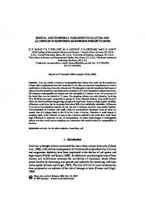
Fig. 3 a Spatial variation in drainage density b Minimum, median and maximum value of groundwater level in low, moderate and high drainage density zones

J Indian Soc Remote Sens

and weathering. The thickness of the highly weathered granite and moderately weathered granite ranges from 11 m to 33 m and from 34 to 77 m respectively. Hydrogeology Groundwater occurs under unconfined condition in the weathered and fractured rocks. Rainfall is the major source of groundwater recharge apart from irrigation returns. Recharge to unconfined aquifers is primarily by downward seepage of rainfall through the unsaturated zone. The groundwater recharge from rainfall varies from 2 % to 10 % (Elango et al. 2012). The depth of dug wells in this area varies from 1.45 m to 15 m. All these wells penetrate till moderately weathered rock. The dug wells are lined only in the soil zone and highly weathered rock zone. Bore wells are of maximum depth of 24 m. Recharge and

Fig. 4 Temporal variation in rainfall and groundwater level in wells located in low, moderate and high drainage density zones

Fig. 5 a Number of observations of groundwater level in different ranges in low, moderate and high drainage density zones b Relation between groundwater level and drainage density in different months

J Indian Soc Remote Sens

abstraction causes rise and fall in water table and in general the groundwater table occur between 0 and 14.6 m below ground level (bgl). In general, the groundwater flow towards southeastern direction in this area (Fig. 2). Drainage Analysis Drainage pattern is the ordered arrangement of streams, which depends on the slope of land, underlying rocks, geological structure, geomorphology and the climatic conditions of an area. The type of drainage pattern and drainage density gives vital information about the characteristics of the terrain and groundwater occurrence. Type of drainage pattern helps to

understand about the slope, intensity of rainfall, nature of the surface material, infiltration capacity, geological structures etc. General types of drainage patterns are dentritic, trellis, radial and rectangular. The study area is dominated by dentritic to subdentritic pattern due to the presence of more or less similar type of rock type. The drainage pattern is fine textured in the southeastern side in comparison to the rest of this area due to more surface water flow towards Pedda Vagu river. Drainage density is defined as the ratio of total length of rivers and streams to the total area considered. Area of high drainage density thus will indicate that most part of the area is covered by drainage and vice versa. Thus the drainage density of an area gives an idea about surface

Table 1 Coordinates, well depth, geology, drainage density and rise in groundwater level Well No

Latitude (decimal)

Longitude (decimal)

Well depth (m)

Rise in groundwater level (m) when rainfall>100 mm

Geology

Drainage density zones Low 1 2 3

16.77 16.74 16.76

78.90 78.90 78.91

7.50 5.53 2.70

4 5 7 8 9 10 11 13 14 15 16 17 21 22 24 26 28 32

16.66 16.63 16.61 16.61 16.68 16.65 16.67 16.66 16.65 16.63 16.65 16.66 16.73 16.73 16.77 16.72 16.75 16.71

79.16 79.18 79.23 79.23 79.26 79.22 79.22 79.17 79.12 79.06 79.03 79.01 78.86 78.84 78.86 78.90 78.94 79.08

7.70 10.50 16.60 16.60 3.58 1.45 10.94 10.45 3.60 10.00 5.20 2.00 9.00 3.30 6.95 2.80 12.45 10.65

33 34 35 38 39 43 44 45

16.69 16.68 16.69 16.70 16.72 16.69 16.63 16.74

79.08 79.10 79.14 79.24 79.11 78.89 79.12 78.90

9.52 3.60 6.10 6.10 11.04 7.21 6.90 10.96

Moderate

High 3.2 0.89 1.5

5.02 4.18 14.42 12.27 2.51 2.7 4.6 6.9 2.2 4.1 0 0 3.65 1.6 6.8 0 7.55 6.82 2.95 3.29 2.27 2.3 5.2 2.12 6.6 6.44

Grey biotite granite Grey biotite granite Grey biotite granite Grey biotite granite Grey biotite granite Quartzite Quartzite Migmatite granite Grey biotite granite Grey biotite granite Grey biotite granite Grey biotite granite Grey biotite granite Grey biotite granite Grey biotite granite Grey biotite granite Pink biotite granite Grey biotite granite Grey biotite granite Grey biotite granite Grey biotite granite Grey biotite granite Migmatite granite Grey biotite granite Migmatite granite Grey biotite granite Grey biotite granite Grey biotite granite Grey biotite granite

J Indian Soc Remote Sens

flow and the amount of infiltration. In a hard rock terrain, drainage density is considered as one of the prime indicators of groundwater potential and indirectly helps in understanding the porosity and permeability of terrain (Vasanthavigar et al. 2011). In the present study, drainage density was calculated by dividing the area into square cells of 1 km2. The total length of streams in each cell was measured which was divided by 1 km2. The plot of number of cells with different ranges of drainage density follows normal distribution (Fig. 3a). Based on this distribution the area was classified into different drainage density zones as low (2.39 km-1) drainage density. Figure 3a indicates that most of the area is covered by moderate drainage density zones. The range and median values of groundwater level, recorded in wells located in low, moderate and high drainage density are given in Fig. 3b. The maximum groundwater level observed in low, moderate and high drainage density zones are 14.6 m, 10.7 m and 12.0 m bgl respectively during the period of this study i.e. from March 2008 to January 2010. More groundwater is recharged in low drainage density area due to high infiltration, which is reflected by rise in groundwater level after the rains (Fig. 4). From Fig. 4 it is evident that groundwater recharge is high in low drainage density region during rainfall, compared to moderate and high drainage density regions. This observation indicate that the runoff is more in the moderate and high drainage density regions.

Fig. 6 a Fractures seen in a granitic outcrop near Devarkonda b Picture of dug well no 24 c Rose diagram of fractures

Further, the number of groundwater level observations were compared with the drainage density in Fig. 5a. The number of observations made with groundwater level in different ranges are high in the low drainage density zone. The groundwater level measured in a well and drainage density of that location was compared in different months. The drainage density versus groundwater level in the study area in four different months are shown in Fig. 5b. This figure shows that, in general groundwater level is deep in regions with high drainage density. Based on the analysis of groundwater levels, it is understood that groundwater occurs at shallow depths in regions with low drainage density. In general, in wells of low drainage density zones, groundwater level increase is more when compared to those of moderate and high drainage density zones, when monthly rainfall is greater than 100 mm (Table 1). The lesser rise in groundwater level in moderate and high drainage density zones are due to higher runoff and less groundwater recharge. This is also supported by temporal groundwater level fluctuation in wells located in low, moderate and high drainage density zones and rainfall in the area (Fig. 4). Lineament Analysis Lineament is a linear feature of regional extent, many a times it indicates the lithological contacts and underlying geological structure. Acharya and Mallik (2012) visually interpreted the lineaments from IRS-P6 LISS III standard False Color Composite (FCC) imageries treating the lineaments literally as straight lines in the horizontal plane in 1:50,000 scale. The onscreen observations of satellite

J Indian Soc Remote Sens

images, along with the geology (lithological contacts, faults and fractures zones) in the GIS environment helped to identify the linear features (Galanos and Rokos 2006). Study of lineaments is important for identification of groundwater flow paths (Mallast et al. 2011) and it is one of the indicators for groundwater resources (Sander et al. 1997). Hossam et al. (2011) carried out lineament analysis for groundwater exploration, as the joints and fractures serve as conduits for movement and storage of groundwater. Lineaments in the study are due to the fractures, faults and dykes. Fractures Fracture is any local separation or discontinuity in a geological formation. Fractures in rocks are formed due to compressional or tensional stress which exceeds the strength of the rock. Sometimes it forms deep fissures or

crevice in the rock. Presence of fractures increases the rate of weathering which in turn increases the porosity and permeability of the rocks. Barton et al. (1995) studied the relationship between the locally concentrated fluid flow, the orientation and relative aperture of fractures. High fracture density and fracture intersection are the most significant areas of groundwater occurrence (Magowe and Carr 1999). As fractures are minor structures they were studied by geological field investigation in the study area. Fractures seen on the outcrops, excavations and well sections (Fig. 6a & b). The direction and frequency of fractures are shown as a rose diagram (Fig. 6c). This diagram indicate that most of the fractures are trending NNESSW and NS. The number of fractures trending in other directions are relatively less. Field observation indicates, NS trending fractures occur at intervals of about 10 cm to 30 cm. On the other hand fractures which trend along EW

Fig. 7 a Spatial variation in dyke density with rose diagram b Dolerite dyke seen in a cross section of road cutting to Peddagattu c Minimum, median and maximum value of groundwater level in low, moderate and high dyke density zones

J Indian Soc Remote Sens

are at distances greater than 80 cm. Majority of these fractures are steeply dipping with dip angle greater than 80º. Further, horizontal fractures are also present at distances from 30 cm to 60 cm, which can be observed in well sections and excavations. Dykes Dykes are vertical or steeply dipping igneous intrusives. This area is traversed by number of dolerite dykes. Dolerite dykes totalling 217 and 5 faults where identified and mapped (Fig. 7a). The length of these dykes ranges from 0.17 km to 10.23 km whereas most of the dykes are of length steeply dipping or vertical. Dolerite dyke seen in a road cutting is shown in Fig. 7b. Rose diagram was prepared to understand the orientation and number of dykes (Fig. 7a). Majority of the dykes in the study area are trending in EES-WWN and EW direction. Around 26 dykes are trending in N-S direction. The dykes are generally considered as impermeable and hence they are likely to function as barriers for groundwater flow. Dyke density was calculated to understand its influence on groundwater level fluctuation. This is the ratio of total length of the dykes in each cell divided by the cell area. The area was divided into square cells of 1 km2 and the total length of dykes passing in each cell was measured to estimate dyke density. Dyke density map of this area was prepared in order to study the impact of dykes on groundwater level fluctuation. The study area was divided into three zones as low, moderate and high dyke density by dividing the range of dyke density from 0 to 2.96 km-1 at natural breaks. It is based on the subjective recognition of gaps in the number of distribution of cells, where there are significantly lesser observations. Plotting a histogram of the data can identify these gaps and this method minimizes variation within classes and maximizes variation between classes. Also, it is most useful when the data set has more than one modal value. As the numbers of dykes present in this region is less and they are not uniformly distributed over the entire area, the natural breaks method was used to classify the region as low (< 0.39 km-1), moderate (0.39 km-1 to 1.08 km-1) and high (>1.08 km-1) and their spatial distribution is shown in Fig. 7a. The range of groundwater level variations and the median value of wells located in low, moderate and high density zones are given in Fig. 7c. The maximum groundwater level observed in low, moderate and high density zones are 14.4 m, 12.0 m and 10.4 m bgl respectively. This figure shows that there is no significant variation in groundwater level in low, moderate and high dyke density areas. No major difference in the number of observations of groundwater level in different ranges in the low, moderate and high dyke density zones as

Fig. 8 a Number of observations of groundwater level in different ranges in low, moderate and high dyke density zones b Relation between groundwater level and dyke density in different months

J Indian Soc Remote Sens

shown in Fig. 8a. Even in the region with high dyke density, groundwater occurs at shallow depths. There is no difference in groundwater level observations in the low, moderate and high dyke density zones as seen in Fig. 8b, which indicate that the dykes are not affecting groundwater flow. Temporal groundwater level variation along with rainfall (Fig. 9a) indicates that there is no major difference in groundwater level fluctuation among the wells located in low, moderate and high dyke density areas. Similarly the pattern of fluctuation of groundwater level in wells located in these three different dyke density zones is similar. Further, the variation in groundwater level with respect to time in the wells located across the dolerite dykes are similar (Fig. 9b). This also indicate that the dykes are not functioning as a barrier to groundwater flow in this area. Further, the EC of groundwater measured during a field visit on 16th June 2011 across a dyke which was 1,053 μS/cm and 1,033 μS/cm. The groundwater level was same across this dyke. As EC value and groundwater level of

these two wells are similar, the dykes are not functioning as a barrier to groundwater flow. As majority of fractures in the rocks of the region (Fig. 6c) are oriented in a direction opposite to that of dykes (Fig. 7a), the dykes are not functioning as a barrier and altering the general groundwater flow direction especially as the groundwater occurs at relatively shallow depth in the region. Rajesh et al. (2012) also support this fact that dykes are not acting as a barrier to groundwater flow in this area. The depth up to which the dykes are weathered and fractured will be much greater than the depth of the groundwater table. Field investigation also revealed the presence of horizontal joints in the dykes. A weathered and dissected dolerite dyke is shown in Fig. 10a. All these indicate that the groundwater occurring around the dykes are not compartmentalized especially at the top of the saturated zone. However, it is probably compartmentalized at greater depths where the dolerite intrusives are massive. The conceptual diagram is given in Fig. 10b to illustrate this. As this study is based on

Fig. 9 a Temporal variation in rainfall and groundwater level in wells located in low, moderate and high dyke density zones b Temporal variation in groundwater level (msl) in wells across the dykes

J Indian Soc Remote Sens Fig. 10 a Weathered and dissected dolerite dyke observed in the field b Conceptual cross section across a dolerite dyke

the groundwater level observations made in the existing wells of depth less than 17 m, deeper aquifer system if any this region could be considered.

Conclusion The presence of drainage and dyke and their impact on groundwater level fluctuation were studied in a hard rock terrain of south India. The quantity and flow of groundwater in this region is predominantly controlled by the intensity of weathering, drainage density and presence of fractures. The drainage density plays a major role on the groundwater level fluctuation. Groundwater level fluctuation is high in low drainage density region. There is a significant rise in groundwater level in the regions of low drainage density after rainfall than the moderate and high density regions. The dolerite intrusives are not functioning as a barrier to the groundwater flow and this is due to the presence of major fractures and the due to high intensity of weathering. Hence, the mere presence of dolerite dykes could not be considered to be a barrier for groundwater flow. Similarly depth of groundwater table is not related to the density of dykes, indicating groundwater zone is not compartmentalized in this area especially at shallow depths. Thus the study highlights that the drainage density plays a major role in groundwater level fluctuation and as the dykes are weathered, they do not affect the groundwater flow in this shallow unconfined aquifer. This may be the case in

most of the other regions comprising of crystalline rocks where groundwater occur at shallow depths of less than 15 m. Acknowledgments The authors acknowledge the Board of Research in Nuclear Sciences, Department of Atomic Energy, Government of India for funding this work (Grant no. 2007/36/35). Authors also thank the Department of Science and Technology’s Funds for Improvement in Science and Technology scheme (Grant No. SR/FST/ESI-106/2010) and University Grants Commission’s Special Assistance Programme (Grant No. UGC DRS II F.550/10/DRS/2007(SAP-1)) for their support in creating laboratory facilities, which helped in carrying out part of this work.

References Acharya, T., & Mallik, S. B. (2012). Analysis of lineament swarms in Precambrian metamorphic rocks in India. Journal of Earth System Science., 121(2), 453–462. Babiker, M., & Gudmundsson, A. (2004). The effects of dykes and faults on groundwater flow in an arid land: the Red Sea Hills, Sudan. Journal of Hydrology, 297, 256–273. Ballukraya, P. N., & Kalimuthu, R. (2010). Quantitative hydrogeological and geomorphological analyses for groundwater potential assessment in hard rock terrains. Current Science, 98(2), 253–259. Barton, C. A., Zoback, M. D., Moos, D., & Sass, J. H. (1995). In situ stress and permeability in fractured and faulted crystalline rocks, Rock mechanics, Daemen &Schultz Central Ground Water Board. (2007). Ground water information Nalgonda district, Andhra Pradesh. Publishing cgwb http:// cgwbgovin/DistrictProfile/AP/Nalgonda.pdf.

J Indian Soc Remote Sens Devi, S. P. D., Srinivasulu, S., & Raju, K. (2001). Hydrogeomorphological and groundwater prospects of the Pageru river basin by using Remote sensing data. Environmental Geology, 40, 1088–1094. Elango, L., Brindha, K., Kalpana, L., Sunny, F., Nair, R. N., & Murugan, R. (2012). Modelling of groundwater flow and transport of radionuclides around a proposed uranium tailings pond. Hydrogeology Journal. doi:10.1007/s10040-012-0834-6. Evans, J. P., Forster, C. B., & Goddard, J. V. (1997). Permeability of faultrelated rocks and implications for hydraulic structure of fault zones. Journal of Structural Geology, 19(11), 1393–1404. Galanos, I., & Rokos, D. (2006). A statistical approach in investigating the hydrogeological significance of remotely sensed lineaments in the crystalline mountainous terrain of the island of Naxos, Greece. Hydrogeology Journal, 14, 1569–1581. Gawande, R., Srivastava, A. K., & Jeyaram, A. (2002). Geological, geomorphological, hydrogeological and land use/land cover studies around Kamthi area, Nagpur district, Maharashtra using remote sensing techniques. Journal of the Indian Society of Remote Sensing, 30(1&2), 95–104. Geological Survey of India. (1995). Geology and minerals map of Nalgonda district, Andhra Pradesh, India Gustafson, G., & Krasny, J. (1994). Crystalline rock aquifers: their occurrence, use and importance. Applied Hydrogeology, 2, 64–75. Henriksen, H. (1995). Relation between topography and well yield in boreholes in crystalline rocks, Sogn og Fjordane, Norway. Groundwater, 33(4), 635–643. Henriksen, H., & Braathen, A. (2006). Effects of fracture lineaments and in-situ rock stresses on groundwater flow in hard rocks: a case study from Sunnfjord, western Norway. Hydrogeology Journal, 14, 444– 461. Hossam, H., Elewa, A., & Quaddah, A. (2011). Groundwater potentiality mapping in the Sinai Peninsula, Egypt, using remote sensing and GIS-watershed-based modeling. Hydrogeology Journal, 19, 613– 628. Khan, M. A., & Moharana, P. C. (2006). Prospecting groundwater resources using RS-GIS—a case study from arid western Rajasthan of India. Journal of the Indian Society of Remote Sensing, 34(2), 171–178. Magowe, M., & Carr, J. R. (1999). Relation between lineaments and Groundwater occurrence in western Botswana. Groundwater, 37(2), 282–286. Mallast, U., Gloaguen, R., Geyer, S., Odiger, T. R., & Siebert, C. (2011). Semi-automatic extraction of lineaments from remote sensing data and the derivation of groundwater flow-paths. Hydrology Earth System Science Discuss, 8, 1399–1431. Mondal, S., Pandey, M. A. C., & Garg, R. D. (2007). Groundwater prospects evaluation based on hydrogeomorphological mapping using high resolution satellite images: a case study in Uttarakhand. Journal of the Indian Society of Remote Sensing, 36, 69–76. Nag, S. K. (2005). Application of lineament density and hydrogeomorphology to delineate groundwater potential zones of

Baghmundi block in Purulia district, West Bengal. Journal of the Indian Society of Remote Sensing, 33(4), 521–529. Neves, M. A., & Morales, N. (2007). Structural control over well productivity in the Jundiaí river catchment, southeastern Brazil. Annals of the Brazilian Academy of Sciences, 79(2), 307–320. Nilsen, K. H., Sydnes, M., Gudmundsson, A., & Larsen, B. T. (2003). How dykes affect groundwater transport in the northern part of the Oslo Graben, EGS—AGU—EUG Joint assembly. Abstracts from the meeting held in Nice, France, pp. 6–11. Perrin, J., Ahmed, S., & Hunkeler, D. (2011). The effects of geological heterogeneities and piezometric fluctuations on groundwater flow and chemistry in a hard-rock aquifer, southern India. Hydrogeology Journal. doi:10.1007/s10040-011-0745-y. Rajesh, R., Brindha, K., Murugan, R., & Elango, L. (2012). Influence of hydrogeochemical processes on temporal changes in groundwater quality in a part of Nalgonda district, Andhra Pradesh, India. Environmental Earth Sciences, 65, 1203–1213. Rao, S. N. (2006). Groundwater potential index in a crystalline terrain using remote sensing data. Environmental Geology, 50, 1067–1076. Rao, N. S., & Reddy, R. P. (1999). Groundwater prospects in a developing satellite township of Andhra Pradesh, India using remote sensing techniques. Journal of the Indian Society of Remote Sensing, 27(4), 193–203. Rao, N. S., Chakradhar, G. K. J., & Srinivas, V. (2001). Identification of groundwater potential zones using remote sensing techniques in and around Guntur town, Andhra Pradesh, India. Journal of the Indian Society of Remote Sensing, 29(1&2), 69–78. Rushton, K. R., & Weller, J. (1985). Response to pumping of a weathered-fractured granite aquifer. Journal of Hydrology, 80 , 299–309. Sander, P., Minor, T. B., & Chesley, M. M. (1997). Groundwater exploration based on lineament analysis and reproducibility test. Groundwater, 35(5), 888–894. Thakur, G. S., & Raghuwanshi, R. S. (2008). Perspect and assessment of groundwater resources using remote sensing techniques in and around Choral river basin, Indore and Khargone districts, MP. Journal of the Indian Society of Remote Sensing, 36, 217–225. Vasanthavigar, M., Srinivasamoorthy, K., Vijayaragavan, K., Gopinath, S., & Sarma, S. (2011). Groundwater potential zoning in Thirumanimuttar sub-basin Tamil Nadu, India—a GIS and remote sensing approach. Geo-spatial Information Sciences, 14(1), 17–26. Vijith, H. (2007). Groundwater potential in the hard rock terrain of western Ghats: a case study from Kottayam district, Kerala using ResourceSat (IRS-P6) data and GIS Techniques. Journal of the Indian Society of Remote Sensing, 35(2), 163–171. Vittala, S., Govindaiah, S., & Gowda, H. (2005). Evaluation of groundwater potential zones in the sub-watersheds of north Pennar river basin around Pavagada, Karnataka, India using remote sensing and GIS techniques. Journal of the Indian Society of Remote Sensing, 33(4), 483–493.