Spatial and temporal variation of stream communities in a ... - Core

Spatial and temporal variation of stream communities in a human-affected tropical watershed Ronald Sanchez-Arguello1*, Aydee Cornejo2,3, Richard G. Pearson4 and Luz Boyero4,5 1 2 3 4 5

Ministerio Nacional del Ambiente, Energıa y Telecomunicaciones, Area de Conservacion Tortuguero, Costa Rica Programa Centroamericano de Maestrıa en Entomologıa, Vicerrectorıa de Investigacion y Postgrado, Universidad de Panama, Panama Seccion de Entomologıa, Instituto Conmemorativo Gorgas de Estudios de la Salud, Ave. Justo Arosemena & Calle 35, 0816-02593 Panama, Panama School of Marine and Tropical Biology, James Cook University, Townsville, QLD 4811, Australia Wetland Ecology Group, Donana Biological Station-CSIC, Avda Americo Vespucio s/n, E-41092 Sevilla, Spain Received 2 September 2009; Accepted 18 May 2010 Abstract – We explored the spatial and temporal variability of benthic macroinvertebrate communities (density, taxon richness, evenness and taxonomic composition) in a tropical Panamanian stream that is potentially affected by organic and chemical pollution resulting from human activities. As predicted, pristine headwaters of Site 1, located within the Altos de Campana National Park, showed the lowest macroinvertebrate densities, suggesting an increase in pollution-tolerant taxa at downstream sites located near human settlements and agricultural land. Moreover, Site 1 had higher accumulated taxon richness than downstream sites (except Site 5), although evenness was higher at Site 3. Density and taxon richness were higher and more variable in the dry season, while evenness was only higher in the dry season at Site 1. Multivariate analysis showed that the fauna responded to a natural longitudinal gradient, but there was also a strong water quality signal associated with human settlements. Community composition was related to abiotic variables commonly associated to pollution, such as alkalinity, dissolved solids, phosphates, and total organic carbon. Key words: Stream macroinvertebrates / Panama / spatial variation / seasonality / tropics

Introduction Fresh waters may well be the most endangered ecosystems in the world, but still information on freshwater biodiversity is incomplete in many areas (Boyero et al., 2009), especially at tropical latitudes that support most of the world’s species (Dudgeon, 2006). This knowledge gap inevitably means that management policies and conservation strategies applied to tropical streams have been derived from research in the temperate zone (Wantzen et al., 2006) and that we still have much to learn about the functioning of tropical streams to be able to optimize their conservation (Moulton and Wantzen, 2006). Two of the five major threats to freshwater biodiversity are water pollution and habitat degradation (Dudgeon, 2006). Organic pollution caused by domestic sewage results in water eutrophication, while deforestation along the edges of watercourses often results in increases in *Corresponding author: [email protected]

temperature and sedimentation (Couceiro et al., 2007). Although sediment deposition is a natural process in streams, human land uses cause increased sedimentation, which can have detrimental effects on benthic stream communities. Sediments can bury macroinvertebrates and their habitats and cause the loss of species requiring coarse substrata for attachment or feeding, while they can promote an increase in abundance of burrowing animals (Connolly and Pearson, 2007). While organic pollution is increasingly under control in developed countries, it remains a major problem in most tropical areas, where streams receive direct inputs of municipal sewage, and water treatment is scarce or absent (Thorne and Williams, 1997; Moulton and Wantzen, 2006; Wantzen et al., 2006). Similarly, rapid development in tropical countries in recent decades has led to large-scale land degradation and erosion (Wantzen et al., 2006). Biodiversity has two major components: the number of taxa (richness) and the distribution of taxon abundances within the community (evenness). In streams, an increase

in water pollution and/or sedimentation often causes a decrease in both macroinvertebrate richness and evenness (Margalef, 1983). An increase in macroinvertebrate abundance is usually related to the proliferation of certain tolerant taxa such as Chironomidae or Oligochaeta (Connolly and Pearson, 2007). Changes in taxonomic composition are also a common indicator of community responses to changes in water and habitat quality (Rosenberg and Resh, 1993; Alba-Tercedor, 1996; Posada et al., 2000). We explored variation in density, richness, evenness and taxonomic composition of macroinvertebrate communities along a tropical stream whose headwaters are pristine and located within a national park, subsequently flowing through various human settlements and subject to organic pollution and sedimentation. We predicted that pristine headwater communities would have higher taxonomic richness and evenness than downstream sites, but the latter would have higher densities due to the proliferation of pollution-tolerant taxa. We also explored seasonal variation of communities and predicted that the lower frequency and intensity of spates in the dry season would allow the development of larger communities (higher densities, and higher richness due to a sampling effect) but also promote species dominance (lower evenness). These predictions have been little explored in the tropics despite tropical streams being subject to alarming levels of human alteration (Pringle et al., 2000).

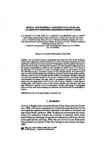
Figure 1. Map of the Capira stream showing the location of the sampling sites (1–6).

Study area The study was conducted at the Capira stream, which arises at 800 m asl at the Cerro Campana, within the Altos de Campana National Park (ACNP), Panama, and flows into the Pacific Ocean (Fig. 1). The climate is tropical humid, characterized by a warm mean annual temperature (24 xC), abundant precipitation (>2500 mm), and mean relative humidity of 80%. Six sampling sites were selected to represent the different conditions found along the stream. Site 1 was located at 743 m asl, within the limits of the ACNP, and thus represented pristine conditions. Sites 2–6 were located at altitudes ranging from 107 to 171 m asl and were potentially affected by agriculture, cattle farming, human settlements and roads (Table 1). Stream habitat was mainly composed of a series of riffles and pools, and substrate was largely composed of gravel, sand and cobble, with abundant leaf litter (mostly in the dry season). Canopy cover ranged from 90 to 95% at Site 1 and 50 to 85% at Sites 2–6 (Table 1).

Material and methods Field and laboratory work

At each site we collected 10 haphazard benthic samples at each of 8 sampling times, 4 in the dry season

(January–April) and 4 in the wet season (May–August) (total number of samples =480) in 2007. Samples were taken using a D-frame net (50 cm width, 250 mm mesh size) and a 50 r 50 cm PVC frame. We placed the net immediately downstream of the frame and without any time limit disturbed the substrate within the frame by hand, so invertebrates were dislodged and carried by the current into the net. The net contents were transferred to a jar and preserved in 70% ethanol. In the laboratory, samples were sorted and macroinvertebrates identified to the lowest taxonomic level possible (mostly genus) using the available literature (Roldan, 1988; Merrit and Cummins, 1996; Springer et al., 2010, unpublished taxonomic keys). At each sampling point we measured current velocity (cm.sx1; averaged from three measurements using a floating cork) and water depth (cm) and recorded the dominant substrate. At each site we estimated qualitatively the % of canopy cover (visually from the middle of the stream), and measured the stream wetted width (m; averaged from three transects at each site) and multiple physico-chemical variables. In situ we measured water temperature, pH and conductivity using a multiparameter Horiba U10. Then we collected water samples and kept them in ice to be transported to the laboratory where we determined biological oxygen demand (BOD), alkalinity, turbidity, hardness, phosphates, nitrates, chlorides, suspended solids (SS), total dissolved solids (TDS)

Intervened Forest 65 ¡ 7.10 107

Human settlement

Intervened Forest Human settlement

13.72 ¡ 7.92 20.84 ¡ 9.89 3.83 ¡ 0.254

9.46 ¡ 0.151

31.55 ¡ 9.97

15.04 ¡ 9.11

Gravel and sand Gravel 69.8 ¡ 5.10 110

Grassland Cattle farming, road 11.1 ¡ 1.14

26.86 ¡ 7.41

13.26 ¡ 7.49

Gravel 63.9 ¡ 4.51 120

Grassland 8.85 ¡ 0.694

34.40 ¡ 8.34

17.17 ¡ 9.72

Sand 57.1 ¡ 10.5 135

16.31 ¡ 8.34 28.63 ¡ 9.71 11.1 ¡ 0.524

Current vel. (cm.sx1) ¡ SE 9.56 ¡ 12.13 Depth (cm) ¡ SE 12.11 ¡ 12.93

6: Villa Camila

5: Villa Rosario

3: Puente Interamericana 4: Puente Capira

2: Pailitas

UTM coord. 618314 N 960341 W 621078 N 963790 W 622569 N 964615 W 624199 N 968340 W 068475 N 095002 W 627415 N 974206 W

Width (m) ¡ SE 1.56 ¡ 1.21

Gravel 63.9 ¡ 6.11 171

Human settlement, agriculture, cattle farming Human settlement, road

Forest type Primary and secondary forest Intervened Forest Human activity None (National Park)

Results

Dominant substrate Gravel Canopy (%) ¡ SE 95 ¡ 0 Altitude (m asl) 743

Data analysis

We determined the main abiotic characteristics of sites, and any environmental gradients, using principal components analysis (PCA), with the correlation coefficient as the dissimilarity measure, in the PC-ORD package (McCune and Mefford, 2006). Variation of the PCA axes explaining most of the variance was explored among sampling sites (1–6) and between seasons (dry/wet), with a two-way analysis of variance (ANOVA) (level of significance a = 0.05) followed by post-hoc Student’s t tests. We characterized macroinvertebrate communities using the following metrics: density (number of individuals per m2, log transformed), richness (number of taxa) and evenness (H'/lnS, where H' = Shannon’s diversity index and S = taxon richness). The spatial and seasonal variation of these metrics was explored with two-way ANOVA (level of significance a = 0.05) followed by posthoc Student’s t tests. Factors were site (1–6) and season (dry/wet). The maximum number of taxa at each site was estimated using jackknife estimates in PCORD (McCune and Mefford, 2006). Variation in taxonomic composition was explored with non-metric multidimensional scaling (NMS) in PC-ORD using the Sorensen (Bray-Curtis) similarity measure. Rare taxa (< 25 individuals in total) were excluded. The NMS was followed by multi-response permutation procedures (MRPP) to test the hypotheses of no differences in taxonomic composition among sites, between seasons and with the interaction site r season. The NMS axes were related to the abundance of each taxon and to biotic and abiotic metrics, including the PCA axis scores, using simple correlations.

Site 1: Rana Dorada

Table 1. Geographic position, altitude, canopy cover, stream wetted width, water depth, current velocity, dominant substrate type, human activity and forest type at each sampling site along the Capira stream.

and total organic carbon (TOC), following the Standard Methods for the Examination of Water and Wastewater (Eaton et al., 1995). All abiotic variables are summarized in Table 2. Average monthly rainfall and temperature data were collected from the closest weather station in Anton (Empresa de Transmision Electrica, 2008); rainfall increased at the end of the dry season (April) and in the wet season (Table 3).

The first three PCA axes summarizing abiotic variation explained the 30%, 15% and 10% of the variance, respectively (eigenvalues: 5.36, 2.67 and 1.88, respectively). Axis 1 was mostly loaded on altitude, canopy, stream width, alkalinity and dissolved solids; axis 2, on water depth, current velocity, pH, BOD, chlorides, nitrates and phosphates; and axis 3, on turbidity. The three axes varied significantly with site and season, and the interaction was significant in all cases (Table 4). Axis 1 differed between Site 1 and the others, and between Site 6 and the others, being similar among Sites 2–5; within sites, Axis 1 differed between the dry and wet seasons only for Site 6. Axis 2

Season Sampling site 1 BOD 1.74 ¡ 1.76 Temperature 21.6 ¡ 1.01 7.77 ¡ 0.58 pH 56.7 ¡ 14.3 Hardness Conductivity 120.8 ¡ 48.2 8.74 ¡ 6.86 Turbidity 22.8 ¡ 1.69 Alkalinity Organic carbon 11.3 ¡ 1.50 Dissolved solids 83.6 ¡ 7.41 16.3 ¡ 16.6 Susp. solids 0.02 ¡ 0.01 Phosphates 0.12 ¡ 0.02 Nitrates 13.3 ¡ 4.40 Chlorides

1.14 ¡ 0.77 26.3 ¡ 0.85 8.28 ¡ 0.33 99.6 ¡ 37.4 177.9 ¡ 24.1 1.76 ¡ 0.23 84.3 ¡ 6.77 12.8 ¡ 1.03 145.8 ¡ 5.54 4.26 ¡ 6.17 0.09 ¡ 0.01 0.05 ¡ 0.02 10.5 ¡ 3.86

2

Dry

4

5

6

1

2

3

Wet

4 5 6 1.26 ¡ 1.11 1.74 ¡ 1.76 1.14 ¡ 0.77 1.26 ¡ 1.11 1.35 ¡ 0.42 0.86 ¡ 0.52 1.13 ¡ 0.68 1.35 ¡ 0.42 0.86 ¡ 0.52 1.13 ¡ 0.68 29.7 ¡ 3.89 21.6 ¡ 1.01 26.3 ¡ 0.85 29.7 ¡ 3.89 26.0 ¡ 1.07 26.8 ¡ 1.54 27.2 ¡ 0.38 26.0 ¡ 1.07 26.8 ¡ 1.54 27.2 ¡ 0.38 7.23 ¡ 0.74 7.77 ¡ 0.58 8.28 ¡ 0.33 7.23 ¡ 0.74 8.42 ¡ 0.50 7.47 ¡ 0.50 7.61 ¡ 0.12 8.42 ¡ 0.50 7.47 ¡ 0.50 7.61 ¡ 0.12 111.6 ¡ 25.9 56.7 ¡ 14.3 99.6 ¡ 37.4 111.6 ¡ 25.9 75.1 ¡ 51.1 101.3 ¡ 13.9 88.9 ¡ 19.6 75.1 ¡ 51.1 101.3 ¡ 13.9 88.9 ¡ 19.6 190.9 ¡ 30.7 120.8 ¡ 48.2 177.9 ¡ 24.1 190.9 ¡ 30.7 167.2 ¡ 58.1 192.9 ¡ 21.3 179.6 ¡ 26.3 167.2 ¡ 58.1 192.9 ¡ 21.3 179.6 ¡ 26.3 9.79 ¡ 1.68 8.74 ¡ 6.86 1.76 ¡ 0.23 9.79 ¡ 1.68 1.51 ¡ 0.18 3.75 ¡ 1.82 8.45 ¡ 4.85 1.51 ¡ 0.18 3.75 ¡ 1.82 8.45 ¡ 4.85 89.7 ¡ 5.61 22.8 ¡ 1.69 84.3 ¡ 6.77 89.7 ¡ 5.61 83.6 ¡ 5.46 87.4 ¡ 4.39 78.2 ¡ 4.01 83.6 ¡ 5.46 87.4 ¡ 4.39 78.2 ¡ 4.01 12.3 ¡ 2.19 11.3 ¡ 1.50 12.8 ¡ 1.03 12.3 ¡ 2.19 13.4 ¡ 2.35 34.9 ¡ 13.3 11.6 ¡ 2.54 13.4 ¡ 2.35 34.9 ¡ 13.3 11.6 ¡ 2.54 156.7 ¡ 4.14 83.6 ¡ 7.41 145.8 ¡ 5.54 156.7 ¡ 4.14 139 ¡ 6.83 141.1 ¡ 10.9 147.1 ¡ 2.06 139 ¡ 6.83 141.1 ¡ 10.9 147.1 ¡ 2.06 5.57 ¡ 3.90 16.3 ¡ 16.6 4.26 ¡ 6.17 5.57 ¡ 3.90 0.88 ¡ 0.67 0.66 ¡ 0.69 6.80 ¡ 3.62 0.88 ¡ 0.67 0.66 ¡ 0.69 6.80 ¡ 3.62 0.21 ¡ 0.04 0.02 ¡ 0.01 0.09 ¡ 0.01 0.21 ¡ 0.04 0.09 ¡ 0.01 0.08 ¡ 0.01 0.03 ¡ 0.00 0.09 ¡ 0.01 0.08 ¡ 0.01 0.03 ¡ 0.00 0.30 ¡ 0.07 0.12 ¡ 0.02 0.05 ¡ 0.02 0.30 ¡ 0.07 0.06 ¡ 0.04 0.06 ¡ 0.03 0.09 ¡ 0.02 0.06 ¡ 0.04 0.06 ¡ 0.03 0.09 ¡ 0.02 15.6 ¡ 1.03 13.3 ¡ 4.40 10.5 ¡ 3.86 15.6 ¡ 1.03 9.88 ¡ 3.59 13.3 ¡ 0.87 14.3 ¡ 1.25 9.88 ¡ 3.59 13.3 ¡ 0.87 14.3 ¡ 1.25

3

Table 2. Abiotic variables measured at each sampling site and season (average ¡ SE). All in ppm except temperature (in xC), pH, and turbidity (in NTU).

Table 3. Average (¡ SD) temperature and rainfall at each sampling time, collected from the closest weather station in Anton (Empresa de Transmision Electrica, 2008). January February March April May June July August

Source Axis 1 Site Season Site r Season Error Axis 2 Site Season Site r Season Error Axis 3 Site Season Site r Season Error

Temperature ( xC) 28.6 ¡ 7.7 28.8 ¡ 9.3 29.4 ¡ 9.3 29.4 ¡ 9.0 28.4 ¡ 8.2 27.6 ¡ 7.5 27.7 ¡ 7.9 27.5 ¡ 7.9 Rainfall (mm) 0.0 ¡ 0.0 0.0 ¡ 0.0 0.0 ¡ 0.0 2.6 ¡ 13.4 4.1 ¡ 6.0 11.5 ¡ 22.0 6.4 ¡ 12.5 8.4 ¡ 15.4

Table 4. Results of ANOVA exploring variation of the principal component analysis (PCA) axes summarizing abiotic variation. ANOVA factors are: sampling site (1–6) and season (dry-wet). Degrees of freedom, sums of squares, F statistic and p-values are shown. df SS F p

5 1 5 36 228.77 14.34 4.55 9.52 173.11 54.25 3.44 < 0.0001 < 0.0001

5 1 5 36 21.75 51.42 19.11 27.72 5.65 71.17 4.96

5 1 5 36 43.00 10.22 18.01 16.25 19.33 6.81

0.0121

< 0.0001

0.0006

0.0015

< 0.0001 < 0.0001

0.0001

separated Sites 1 and 5 from Sites 2–4 and Site 6 from Sites 2–3; within sites, Axis 2 differed between seasons for Sites 3–6. Axis 3 separated Sites 1–4 from Sites 5–6; within sites, Axis 3 differed between seasons for Sites 4 and 6. We collected a total of 25 879 individuals belonging to 121 taxa from 17 orders. Communities were dominated by insects (91.7%) and mollusks (6.87%). The most common orders were Diptera (mainly Chironomidae), Ephemeroptera (mainly Leptohyphidae, Leptophlebiidae, and Caenidae), Mollusca (both Gastropoda and Bivalvia), Trichoptera (mainly Hydropsychidae, Glossosomatidae and Calamoceratidae), Coleoptera (mainly Elmidae) and Odonata (mainly Coenagrionidae and Libellulidae) (online Appendix I, available at www.limnology-journal. org/). Macroinvertebrate densities were lowest at Site 1 (mean of 80 individuals per m2), followed by Site 6 (163), but did not differ significantly among the other four sites (206–301 individuals per m2). Density was higher in the dry season (mean of 328 individuals per m2) than in the wet season (103) and the interaction site r season was

Table 5. Results of ANOVA exploring variation of macroinvertebrate density, taxonomic richness, and evenness. ANOVA factors are: sampling site (1–6) and season (dry-wet). Degrees of freedom, sums of squares, F statistic and p-values are shown. Source Density Site Season Site r Season Error Richness Site Season Site r Season Error Evenness Site Season Site r Season Error

df

SS

F

p

5 1 5 468

22.70 54.85 2.88 134.09

15.84 191.46 2.01

< 0.0001 < 0.0001

5 1 5 468

1696.32 3203.33 274.87 9994.65

15.89 150.00 2.57

< 0.0001 < 0.0001

5 1 5 462

0.70 0.01 0.66 16.48

3.84 0.33 3.63

0.0020 0.5621 0.0031

0.0753

0.0260

Table 6. Jacknife estimates of maximum number of taxa at each sampling site.

Site Site 1 Site 2 Site 3 Site 4 Site 5 Site 6

Total number of taxa 70.0 69.0 65.0 64.0 71.0 62.0

1st order jacknife estimate 89.7 80.8 83.8 80.8 91.7 76.8

2nd order jacknife estimate 98.7 86.8 93.6 89.7 108.4 85.7

nearly significant, differences among sites being more pronounced in the dry season (Table 5, Fig. 2). Macroinvertebrate richness (number of taxa per sample) was lowest at Site 1 (mean of 6 taxa per sample) followed by Site 6 (9), and similar at the other four sites (10–12 taxa per sample) (Table 5, Fig. 2). However, jackknife estimates indicated higher cumulative taxonomic richness at Sites 1 and 5 (Table 6). Richness was higher in the dry season (mean of 12.3 taxa per sample) than in the wet season (7.1) and the interaction site r season was significant, differences among sites being more pronounced in the dry season (Table 3, Fig. 2). Evenness was generally high, but was significantly higher at Site 3 (mean of 0.86) than at Sites 1, 4 and 5 (mean of 0.73–0.78), and significantly lower at Site 5 (mean of 0.73) than at Sites 2, 3 and 6 (means of 0.80– 0.86). Evenness did not vary between seasons, but the interaction site r season was significant: seasonal differences were significant only at Sites 1 (evenness higher in the dry season (mean of 0.84) than in the wet season (mean of 0.72)) and 4 (evenness higher in the wet season (mean of 0.85) than in the dry season (mean of 0.72)) (Table 5, Fig. 2).

Figure 2. Variation among sampling sites and seasons (grey bars: dry season; black bars: wet season) of: 1) macroinvertebrate density; 2) taxonomic richness; and 3) evenness (N = 480).

The NMS (based on 48 taxa, see online Appendix I) was performed using two axes (stress: 0.13). Axis 1 (45% of variance) separated the dry from the wet season, while Axis 2 (44% of variance) separated Sites 1 and 6 from all the other sites (Fig. 3). The MRPP showed a highly significant difference among sites (T = x 9.18, p < 0.0001), with Site 1 differing from all other sites (p < 0.001 in all cases), Site 6 also differing from all other sites (p < 0.050 in all cases), and Site 2 differing from Site 5 (p = 0.003). Differences between seasons and the interaction site r season were also highly significant (T=x 13.27, p < 0.0001; and T= x 10.77, p < 0.0001, respectively).

Table 7. Correlations of the non-metric multidimensional scaling (NMS) axes with taxa. Only significant correlations (p < 0.01) are shown. Taxa NMS axis 1 and: Chironomini Farrodes Tanypodinae Leptohyphes Caenis Baetis Tanytarsini NMS axis 2 and: Tanypodinae Tricorythodes Gastropoda Chironomini Leptohyphes Caenis Bivalvia Macrothemis Vacuperinus Polycentropus Brechmorhoga

Correlation (r)

Taxa

Correlation (r)

0.722 0.635 0.558 0.542 0.531 0.468 0.440

Phylloicus Argia Macronema Tricorythodes Heterelmis Nectopsyche Macrelmis

0.451 0.433 0.432 0.416 0.411 0.379 0.372

0.791 0.790 0.713 0.668 0.622 0.565 0.546 0.546 0.482 0.479 0.459

Austrolimnius Tanytarsini Ceratopogoninae Phylloicus Nectopsyche Macrelmis Farrodes Neoelmis Erpetogomphus Macronema

0.415 0.458 0.453 0.453 0.442 0.440 0.436 0.429 0.398 0.372

Discussion Variation among sites

Figure 3. Non-metric multidimensional scaling showing separation of: A, sampling sites (1–6); and B, seasons (D: dry, W: wet), based on taxonomic composition.

NMS axes were determined by several taxa, indicated by correlations between their log abundance and the axis scores (Table 7). The abundances of various Ephemeroptera (5 taxa), Diptera (3), Coleoptera (3), Trichoptera (2) and Odonata (1) correlated with axis 1; and abundances of various Ephemeroptera (5), Diptera (4), Odonata (4), Trichoptera (3), Coleoptera (3) and Mollusca (2) correlated with axis 2 (Table 7). Axis 1 was related to macroinvertebrate density and richness, and to various environmental variables, including PCA axis 2 and 3, and water depth, current velocity, turbidity and BOD. Axis 2 was also related to macroinvertebrate density and richness and to PCA axis 1 and multiple environmental variables: alkalinity, dissolved solids, altitude, phosphates, current velocity, stream width, conductivity, canopy cover, water depth and TOC (Table 8).

Our results suggested on-going effects of pollution on macroinvertebrate communities in our study stream. As predicted, headwater communities at the pristine Site 1 showed the lowest densities, and the highest taxonomic richness at the site scale (together with Site 5). The other sites, all outside the national park and located near human settlements, roads and agricultural areas, had higher densities and generally lower richness. This could be due to an effect of pollution and/or habitat modification at these impacted sites, as shown for temperate streams (e.g. Pascoal et al., 2001). However, we must be cautious when interpreting differences between Site 1 and downstream sites, as these could also be at least partly due to a natural altitudinal gradient (Site 1 was located at more than 700 m asl while Sites 2–6 were between 100 and 200 m asl). Altitude was one of the abiotic variables most related to variation in macroinvertebrate densities and richness between Site 1 and the other sites. Stream width, which generally co-varies with altitude, was also related to this variation, as well as canopy cover, alkalinity, and dissolved solids. These variables may show some natural variation along an altitudinal gradient (particularly canopy cover) but are also frequently related to human activities (Allan, 2004). Moreover, some other variables commonly associated to organic pollution (pH, BOD, chlorides, nitrates and phosphates) were strongly related to differences in taxonomic richness between Sites 1 and 5 and the other sites.

Table 8. Correlations of the non-metric multidimensional scaling (NMS) axes with community metrics and abiotic variables (including the PCA axes summarizing abiotic variation). Only significant correlations (p < 0.01) are shown. Variables NMS axis 1 and: Density Richness PCA axis 2 Depth Current Turbidity PCA axis 3 BOD NMS axis 2 and: Density Alkalinity Richness PCA axis 1 Dissolved solids Altitude Phosphates Current Width Conductivity Canopy Depth TOC

Correlation (r) 0.7734 0.7287 0.4683 x 0.4106 x 0.3378 x 0.3052 x 0.3011 x 0.2944 0.8412 0.8188 0.7831 0.7737 0.7662 x 0.6763 0.5766 x 0.5236 0.5151 0.4618 x 0.4612 0.3487 0.2874

Other studies have shown natural upstream-downstream gradients in macroinvertebrate communities, but these are usually correlated with changes in substrate particle size along the stream (Vannote et al., 1980). Connolly et al. (2007) found, in streams of the Australian wet tropics, a downstream decline in taxon richness, as well as a longitudinal gradient in macroinvertebrate community composition, both strongly related to substrate particle size. Their study streams were relatively short, with rapid changes in substrate over short distances as a product of high rainfall and steep ranges. In our case, however, there was no clear longitudinal gradient in substrate particle size, and thus natural gradients in taxon richness and community composition are less likely. The taxonomic composition of communities differed at the pristine Site 1, and also at Site 6, and this variation was associated with altitude and related variables such as stream width and water depth, as well as several other variables likely to be related to human influence (canopy cover, dissolved solids, phospates, TOC). Several taxa were absent only at Site 1 (Austrolimnius, Bivalvia, Caenis, Erpetogomphus and Vacuperinus) or scarce at Sites 1 and 6 (Brechnomorga, Cerapogoninae, Macrelmis, Macrothemis, Nectopsyche, Neoelmis, Phylloicus), while other taxa were much more abundant at Sites 2–5 (Chironomini, Leptohyphes) or 2–6 (Tanypodinae, Tanytarsini, Tricorythodes). Many chironomid species are well known to be pollutiontolerant (Pearson and Penridge, 1987). NMS axis 2 was associated mainly with the normal longitudinal turnover of species expected in streams (Connolly et al.,

2007), while NMS axis 1 was clearly associated with water quality parameters, including PCA axes 2 and 3. Thus, even though there was no strong evidence of a pollution fauna (Hynes, 1960), we were able to discriminate between normal gradients and the subtle effects of human activity on the invertebrate assemblages. Seasonal variation

As predicted, macroinvertebrate densities and taxonomic richness were higher in the dry season. Moreover, variation in densities and richness among sites was less obvious in the wet season, which could be due to the dilution effect caused by the increased discharge (Ramirez and Pringle, 2001). Taxonomic composition also varied with season, mostly due to variation in several Diptera, Ephemeroptera, Coleoptera, Odonata and Trichoptera, all of them more abundant in the dry season. Taxonomic variation between seasons was related to water depth, current velocity, turbidity and BOD, factors clearly related to rainfall. Conclusions

Our results suggest that human settlements and activities next to the Capira stream affect the structure and composition of macroinvertebrate assemblages, through changes in habitat characteristics and water chemistry. However, changes are not pronounced and no obvious “pollution fauna” (Hynes, 1960) was evident, unlike the more extreme conditions found in a Queensland tropical stream that received sugar mill wastes (Pearson and Penridge, 1987). Other studies have also found humanrelated impacts on macroinvertebrate assemblage structure and composition in tropical streams, e.g. Matagi (1996) in Uganda, Ndaruga et al. (2004) in Kenya, Helson et al. (2006) in Trinidad or Yule et al. (2010) in Indonesia. However, information available from tropical streams is still relatively scarce, despite rates of habitat degradation and biodiversity loss being exceptionally high in the tropics. Understanding how tropical streams change in response to land use is a major priority for management and conservation of these ecosystems (Boyero et al., 2009) and, while major effects can be obvious (e.g., Pearson and Penridge, 1987), more subtle effects need care in sampling design to remove effects of natural gradients (Connolly et al., 2007). In this study, multivariate analysis showed that the invertebrate assemblages clearly distinguished a natural altitudinal gradient from increases in contaminants caused by human activity. Acknowledgements. The Secretaria Nacional de Ciencia, Tecnologıa e Innovacion (SENACYT) provided financial support and the Smithsonian Tropical Research Institute (STRI) provided facilities. This study was part of RS’s MSc thesis at the University of Panama, funded by a scholarship from Deutscher Akademischer Austausch Dienst (DAAD).

References Alba-Tercedor J., 1996. Macroinvertebrados acuaticos y calidad de las aguas de los rıos, IV Simposio del Agua en Andalucıa (SIAGA). Almaeria, 2, 203–213. Allan J.D., 2004. The influence of land use on stream ecosystems. Annu. Rev. Ecol. Evol. Sys., 35, 257–284. Boyero L., Ramirez A., Dudgeon D. and Pearson R.G., 2009. Are tropical streams really different? J. N. Amer. Benthol. Soc., 28, 397–403. Connolly N. and Pearson R.G., 2007. The effect of fine sedimentation on tropical stream macroinvertebrate assemblages: a comparison using flow-through artificial stream channels and recirculating mesocosms. Hydrobiologia, 592, 423–438. Connolly N.M., Pearson B.A. and Pearson R.G., 2007. Macroinvertebrates as indicators of ecosystem health in Wet Tropics streams. In: Arthington A.H. and Pearson R.G. (eds.), Biological Indicators of Ecosystem health in Wet Tropics Streams, Final Report Task 3 Catchment to Reef Research Program Cooperative Research Centre for Rainforest Ecology & Management and Cooperative Research Centre for the Great Barrier Reef World Heritage Area, 129–176. Couceiro S.R., Hamada N., Luz S.L., Forsberg B.R. and Pimentel T.P., 2007. Deforestation and sewage effects on aquatic macroinvertebrates in urban streams in Manaus, Amazonas, Brazil. Hydrobiologia, 575, 271–284. Dudgeon D., 2006. The impacts of human disturbance on stream benthic invertebrates and their drift in North Sulawesi, Indonesia. Freshwat. Biol., 51, 1710–1729. Eaton A.D., Clesceri L.S. and Greenberg A.E., 1995. Standard Methods for the Examination of Water and Wastewater, 19th edn., American Public Health Association, Washington DC, 1000 p. Empresa de Transmision Electrica S.A., 2008. Registros diarios de temperaturas y humedad relativa de la estacion de Anton, Panama, http://www.hidromet.com.pa/sp/InicioFrm.htm. Helson J.E., Williams D. and Turner D., 2006. Larval chironomid community organization in four tropical rivers: human impacts and longitudinal zonation. Hydrobiologia, 559, 413–431. Hynes H.B.N., 1960. The biology of polluted waters, Liverpool University Press, Liverpool. Margalef R., 1983. Limnologia, Omega, Barcelona, 1010 p. Matagi S.V., 1996. The effect of pollution on benthic macroinvertebrates in a Ugandan stream. Arch. Hydrobiol., 137, 537–549. McCune B. and Mefford M.J., 2006. PC-ORD. Multivariate Analysis of Ecological Data, Version 5.10, MjM Software, Gleneden Beach.

Merrit R.W. and Cummins K.W., 1996. An introduction to the aquatic insects of North America, Kendall/Hunt Publication, Dubuque, 862 p. Moulton T.P. and Wantzen K.M., 2006. Conservation of tropical streams special questions or conventional paradigms? Aquat. Conserv., 16, 659–663. Ndaruga A., Ndiritu G., Gichuki N. and Wamicha W.N., 2004. Impact of water quality on macroinvertebrate assemblages along a tropical stream in Kenya. African J. Ecol., 42, 208– 216. Pascoal C., Cassio F. and Gomes P., 2001. Leaf breakdown rates: a measure of water quality? Int. Rev. Hydrobiol., 86, 407–416. Pearson R.G. and Penridge L.K., 1987. The effects of pollution by organic sugar mill effluent on the macro-invertebrates of a stream in tropical Queensland, Australia. J. Environ. Manag., 24, 205–215. Posada J., Roldan G. and Ramirez J., 2000. Caracterizacion fisicoquımica y biologica de la calidad de aguas en la cuenca Piedras Blancas, Antioquia, Colombia. Rev. Biol. Trop., 48, 59–70. Pringle C.M., Scatena F.N., Paaby-Hansen P. and NunezFerrera M., 2000. River conservation in Latin America and the Caribbean. In: Boon P.J., Davies B.R. and Petts G.E. (eds.), Global Perspectives on River Conservation: Policy and Practice, John Wiley & Sons, Chichester, 41–77. Ramirez A. and Pringle C., 2001. Spatial and temporal patterns of invertebrate drift in streams draining a Neotropical landscape. Freshwat. Biol., 46, 47–62. Roldan G., 1988. Guıa para el estudio de los macroinvertebrados acuaticos del Departamento de Antioquia, Fondo FEN, Medellın, 217 p. Rosenberg D.M. and Resh V.H., 1993. Freshwater biomonitoring and benthic macroinvertebrates, Chapman and Hall publishers, New York, 488 p. Springer M., Hanson P. and Ramirez A. (eds.), 2010. Macroinvertebrados de Agua Dulce de Costa Rica I. Rev. Biol. Trop., 58, Suppl. 3. Thorne R. and Williams W., 1997. The response of benthic macroinvertebrates to pollution in developing countries: a multimetric system of bioassessment. Freshwat. Biol., 37, 671–686. Vannote R.L., Minshall G.W., Cummins K.W., Sedell J.R. and Cushing C.E., 1980. The river continuum concept. Can. J. Fish. Aquat. Sci., 37, 130–137. Wantzen K.M., Ramirez A. and Winemimller K.O., 2006. New vistas in Neotropical stream ecology – Preface. J. N. Amer. Benthol. Soc., 25, 61–65. Yule C.M., Boyero L. and Marchant R., 2010. Effects of sediment pollution on food webs in a tropical river (Borneo, Indonesia). Mar. Freshwat. Res., 61, 204–213.