Spatial and temporal variations in copepod community structure in the ...

MARINE ECOLOGY PROGRESS SERIES Mar Ecol Prog Ser

Vol. 230: 211–224, 2002

Published April 5

Spatial and temporal variations in copepod community structure in the lower St. Lawrence Estuary, Canada Stéphane Plourde1,*, Julian J. Dodson1, Jeffrey A. Runge2, Jean-Claude Therriault2 1

Département de Biologie, Université Laval, Pavillon Vachon, Ste-Foy, Québec G1K 7P4, Canada Fisheries and Oceans, Maurice-Lamontagne Institute, Division of Ocean Sciences, 850 route de la Mer, Mont-Joli, Québec G5H 3Z4, Canada

2

ABSTRACT: The lower St. Lawrence estuary (LSLE) is a narrow and deep basin under the influence of both estuarine and marine processes. As a result, the LSLE is characterized by strong spatiotemporal heterogeneity in biological and physical environmental conditions. Previous studies have indicated a bias in the summer composition of the copepod population for predominance of late-development stages of Calanus spp., in comparison with adjacent waters of the Gulf of St. Lawrence (GSL) and northwest Atlantic. In this study, we use a 22 mo spatial survey of the LSLE to determine spatial and temporal variations in the copepod community and the relative contribution of Calanus spp. (C. finmarchicus and C. hyperboreus). Multivariate analysis revealed 4 copepod assemblages associated with seasonal patterns in temperature and chlorophyll a. Calanus spp. dominated the early summer community whereas the seasonal increase in abundance of the more surface-dwelling species (Acartia spp., Oithona spp. and Pseudocalanus spp.) explained the mixed Calanus spp./surface species community observed in late summer-autumn and winter. Three recurrent geographic zones can be discriminated in the LSLE on the basis of specific composition and abundance. The copepod community in the upper-central Laurentian Channel was dominated by Calanus spp. Downstream, in late summer-autumn and winter, a mixed Calanus/surface species assemblage was observed. In the shallow region, a very low abundance of Calanus spp. resulted in dominance of surface species after the early summer period. The genus Calanus spp. was the dominant component of the copepod community in LSLE as a whole because of its consistently high abundance along the Laurentian Channel during different seasons. A change in environmental conditions in the 1990s associated with a decadal climate variation in the GSL-LSLE region appears to be related to a dramatic increase in abundance of midwater copepod species (mainly Metridia longa) and, subsequent decline in the relative abundance of Calanus spp. We develop the hypothesis that the observed patterns in copepod species composition in the LSLE are primarily a consequence of the combined effect of the export in the residual surface outflow of early life stages of Calanus spp. and small surface-dwelling species and the upstream advection of late-development stages of Calanus spp. and midwater species in the inflowing deep water of the Laurentian Channel. KEY WORDS: Copepod · Community · Spatial · Seasonal · Decadal · Variation · Circulation · Estuary Resale or republication not permitted without written consent of the publisher

INTRODUCTION Seasonal and spatial variations in abundance and composition of zooplankton communities are determined by the interplay between species life cycle *E-mail: [email protected] © Inter-Research 2002 · www.int-res.com

characteristics and environmental conditions. For example, the seasonal succession of species of planktonic copepods has been related to differential timing in reproduction; some species are dependent on the spring phytoplankton bloom, whereas reproduction in others is associated with warmer, post-bloom conditions in summer (Davis 1987, McLaren et al. 1989).

212

Mar Ecol Prog Ser 230: 211–224, 2002

Environmental conditions and animal behaviors also play a key role in the determination of the spatial pattern of zooplankton communities. In estuaries, different zooplankton assemblages have been associated with strong salinity gradients in which resident zooplankton species exhibit specific vertical migration and reproductive strategies in order to maintain a population in these strong advective environments (Laprise & Dodson 1994, Katajisto et al. 1998, Kimmerer et al. 1998). The invasion of shallower coastal regions by the dominant Calanus spp. in late winter appears to be controlled by the interaction between the ascent of adult females to the surface layer and advection in surface currents, whereas advection and aggregation of zooplankton biomass in fjords and at channel heads are determined by the interaction between the vertical distribution of zooplankton and the general circulation pattern (Falkenhaug et al. 1995, Miller et al. 1998, Heath et al. 1999, Lavoie et al. 2000). Finally, deep-water exchanges driven by atmospheric and oceanographic processes often control the seasonal pattern in abundance of Calanus spp. and Metridia spp. in fjords (Aksnes et al. 1989, Osgood & Frost 1996). The lower St. Lawrence estuary is a large marine estuary (200 km long and 20 to 40 km wide) characterized by strong spatiotemporal variation in physical and biological conditions. Its predominant features are the Laurentian Channel (LC), a deep (up to 350 m) marine valley extending unobstructed from the margin of the continental shelf to the head of LSLE, and a permanent cold intermediate layer (CIL) (30 to 125 m) formed by the autumn-winter cooling and mixing and advection of arctic water (Gilbert & Pettigrew 1997). The LSLE has a typical estuarine 2layer circulation in which the intensity of both residual outflow in the upper 0 to 75 m and upward advection of water below 75 m through the Laurentian Channel is driven by the seasonal pattern in freshwater runoff from the St. Lawrence River (see Fig. 1) (Tee & Lin 1987). The seasonal surface circulation pattern is not well described, and its mechanisms of control not fully understood. As surface currents are predominantly outward in the upstream half of the LSLE, the high internal Rossby number in its downstream region allows the formation of semi-permanent mesoscale features (Ingram & El-Sabh 1990). The freshwater runoff appears to control the surface circulation pattern on a seasonal time scale, as suggested by the switch following the decrease in freshwater runoff in late July from an anti-cyclonic (see Fig. 1) to a cyclonic gyre accompanied by the advection of surface water from the Gulf of St. Lawrence (GSL) (Ingram & El-Sabh 1990). The high freshwater runoff in spring-early summer and

this spatiotemporal heterogeneity in surface circulation and hydrographic conditions are responsible for the late onset of the phytoplankton bloom in late June and the regional and temporal variation in phytoplankton biomass and production cycles in the region (Therriault & Levasseur 1985, Zakardjian et al. 2000). Interannual and interdecadal variations in physical conditions have been described in the GSLLSLE, whereas the region underwent a dramatic cooling in the 1990s, as evidenced by the temperature and thickness of the CIL being respectively lower and greater than their long-term averages (Gilbert & Pettigrew 1997). The summer composition of the copepod population in the LSLE is biased towards a dominance of latedevelopment stages of Calanus spp. (55 to 60% of the community) in comparison to adjacent waters of the GSL and northwest Atlantic (Runge & Simard 1990, de Lafontaine et al. 1991). Runge & Simard (1990) hypothesized that this unusual copepod species composition results from the combined effect of the export in the residual surface outflow of early life stages of Calanus spp. and small surface-dwelling species and the upstream advection of late-development stages of Calanus spp. in the inflowing deep water of the LC. They also proposed that the relatively cold surfacewater temperature in summer (3 to 11°C) and the delayed phytoplankton bloom probably hinder local copepod production and development and reinforce the susceptibility of surface-dwellers to being exported. The observations on which the above analysis is founded, however, are derived from a relatively small number of samples taken between May and September and limited to the upstream half of the LSLE. With the objective of understanding the variability in copepod abundance and composition and the influence of physical factors in a dynamic coastal environment, we describe here spatial and temporal patterns of copepod abundance and composition based on a far more complete dataset, gathered over a period of 22 mo and covering the entire LSLE. We examine different spatial and temporal groups revealed by multivariate numerical analyses in order to test the robustness of the assumption of a particularly strong dominance of Calanus spp. in this region. We discuss and develop the coupled advection-life history hypothesis put forward by Runge & Simard (1990) to take into account the more complex patterns emerging from this detailed dataset. Finally, we investigate potential climate-related changes in copepod community structure by comparing the abundance and the composition of the copepod community during summer in the central LSLE before and during a recent cooling event.

Plourde et al.: Copepod community variation in St. Lawrence Estuary

MATERIALS AND METHODS Sampling. A grid of 29 stations distributed along 8 transects located between the head and the mouth of the LSLE was visited on 16 occasions between March 1979 and December 1980 (Fig. 1). Cruises usually took place during the first half of the month and 6 to 9 d were necessary to cover the entire grid. Zooplankton samples were collected with a 0.5 m diameter Bongo net equipped with 150 µm nets, and the volume of water filtered was measured with a flowmeter (General Oceanic) mounted in the mouth of each net. The net was obliquely towed at a ship speed of 2 knots from the surface to a depth of 30 to 250 m, depending on the station depth. Additionally, a vertical tow (250 m to surface) with a 1 m diameter, 158 µm mesh ring net equipped with a TSK flowmeter was made on 10 occasions between June and September 1994 (in addition to the basic protocol and other samples) as described in Plourde et al. (2001). Zooplankton samples were preserved in 4% formalin. Methods for the environmental data measurements during the synoptic sampling of 1979 to 1980 are described in Therriault & Levasseur (1985). Briefly, water samples were collected with 5 l Niskin bottles at depths corresponding to 100, 60, 30, 16 and 1% of the surface incident radiation and, depending on the station depth, at fixed depths of 25, 50, 100, 150, 200 and 250 m below the photic zone. Temperature and salinity profiles were recorded using either a bathythermogragh (in 1979) or a self-contained Bissett-Berman

Fig. 1. Map of the Lower St. Lawrence Estuary (LSLE) and the Gulf of St. Lawrence (GSL) showing the general surface circulation pattern (arrows) in the LSLE in early summer and the Laurentian Channel (LC) identified by the 200 m isobath (closed line) (adapted from El-Sabh 1979). Upperright inset: position of the stations sampled in 1979–1980 (circles) and 1994 (square); open symbols denote stations used in the interdecadal comparison. Lower-right inset: representative depth profile of along-channel baroclinic velocities, U, showing the downstream (positive) and upstream (negative) residual currents in the central LSLE in summer (adapted from Zakardjian et al. 1999)

213

thermosalinograph Model 5580 (in 1980). Additionally, salinity and temperature were measured on sub-samples of water collected with bottles at discrete depths. Technical details on measurements of chlorophyll a (chl a) and particulate organic carbon (POC) concentrations are given in Therriault & Levasseur (1985). We use the RIVSUM index (Budgen et al. 1982) as an index of the freshwater discharge of the St. Lawrence watershed in the LSLE. Data were obtained (from D. Gilbert, Maurice-Lamontagne Institute, Mont-Joli) as monthly means (m3 s–1) of the sum of freshwater discharge from the St. Lawrence River at Cornwall (Ontario), and the Ottawa and Saguenay rivers (Québec). Zooplankton sample analysis. The formalin-preserved zooplankton samples were analyzed in 2 steps. First, the samples were rinsed in tap water and larger organisms such as medusa, euphausiids, mysiids and fish larvae were counted and removed. Second, samples were fractionated with a Folsom splitter (1979 to 1980) or a 10 ml Stemple pipette (1994) in order to arrive at 300 to 600 individuals identified in each subsample. These 2 techniques showed similar coefficient of variation in subsampling the copepod fraction (van Guelpen et al. 1982). No less than 1/100 of the original sample was analyzed. Calanus glacialis was not distinguished from the much more abundant C. finmarchicus in the analysis of samples collected in 1979 and 1980; therefore the 2 species are considered as a single taxon. Data analysis. Multivariate analyses were carried out to objectively identify the spatiotemporal variabil-

214

Mar Ecol Prog Ser 230: 211–224, 2002

ity in copepod species assemblages and to determine the extent of covariation with environmental variables. Samples were first represented by the abundance of the 8 most dominant copepod species or genera (Calanus finmarchicus, C. hyperboreus, Metridia longa, Microcalanus spp., Pseudocalanus spp., Scolecithricella spp., Acartia spp., and Oithona spp.) Seven copepod taxa (Bradidyus similis, Centropages hamatus, Eurytemora spp., Euchaeta norvegica, Metridia lucens, Oncea spp. and Temora longicornis) were excluded from the analysis because of their very low abundance and occurrence (representing 2% of the overall abundance). The abundance data include all copepodite stages sampled with the 150 µm net and were normalized using a log(x + 1) transformation in order to conserve zero values. The first step of the analysis was to identify homogeneous periods based on the monthly averaged (16 mo

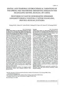
total) abundance of the copepod taxa. From the results of this analysis, the averaged abundance for each station within each period (25 to 29 stations) was computed and the same analysis performed to identify homogeneous groups of stations within each period. The log-transformed abundance data were used to build a similarity matrix (Legendre & Legendre 1998), in which differences between the most abundant species contribute more to the similarity among months or stations than do differences among rarer species. The hierarchical agglomerative clustering model of Lance & Williams (1967; flexible grouping with beta = 0.5) was used to group months or stations into homogeneous clusters. Clusters were then superimposed on a projection in the reduced plane of the first 2 axes of a principal coordinate analysis to separate groups with similar copepod composition. Spearman correlations were calculated between principal axes and abundance data to identify species that contributed the most to the formation of each seasonal and spatial group. The spatial analysis was constrained with the geographic position of the stations (latitude, longitude), allowing smoother clustering that avoids sampling artifacts and less variable solutions that are more readily interpretable (Legendre & Legendre 1998). The more distant the stations, the more similar they must be in order to be grouped together (Legendre & Legendre 1998). Finally, multivariate discriminant analyses were conducted to separate groups on the basis of environmental variables, including salinity, temperature, chl a and POC. Because water samples were collected at various depths in the photic layer throughout the sampling program, averaged values of each parameter in 4 different depth layers were computed: the surface (0 to 3 m), the thermocline (4 to 25 m), the CIL (26 to 100 m) and the deep layer (>100 m). All multivariate numerical analysis were performed with the SAS statistical package (SAS Institute Inc. 1998). The spatiotemporal variation in Calanus spp. contribution to the copepod population was investigated using Fig. 2. Day (open) and night (shaded) vertical distributions of Calanus spp. the averaged absolute and relative (C. finmarchicus, C. hyperboreus), midwater species (Metridia longa, Microcalanus spp., Scolecithricella spp.) and surface species (Acartia spp., Oithona copepod abundances for the periods spp., Pseudocalanus spp.) in late May-early June (top), late June-early July and the regions determined with the (middle) and September (bottom). Data represents means of 2 to 8 oblique vermultivariate analysis. Copepod genera tical tows taken with a BIONESS multinet sampler. Broken lines: 75 m depth; and species were grouped into 3 catevalues inside graphs: integrated mean abundance (ind. m–2) of each copepod categories (J.A.R. et al. unpubl.) gories: (1) Calanus spp. (C. finmarchicus


and C. hyperboreus), (2) midwater species (Metridia longa, Microcalanus spp. and Scolecithricella spp.), and (3) surface species (Acartia spp., Oithona spp. and Pseudocalanus spp.). The latter 2 categories are based on the general vertical distribution of these genera in the LSLE (late May to September), as they were mainly associated with water below and above 75 m respectively (Fig. 2) (J.A.R. et al. unpubl. data). Analysis of variance was performed on normalized data [log(x + 1)] with the STATVIEW statistical package to test for significant spatiotemporal differences in the abundance and relative contribution of Calanus spp. in the region. Comparison of summer composition between decades. We used data collected from June to October to compare the copepod species composition between 1979–1980 and 1994. We considered 3 stations of the 1979–1980 project, as they were located in the vicinity of the monitoring station visited in 1994 (Fig. 1). Average abundance of each copepod class for each period was calculated and compared with a chi-square test to detect significant difference in species composition using the STATVIEW statistical package. Correction of abundance data according to depth sampled. During the synoptic sampling of 1979 and 1980 and the 1994 monitoring effort, the deep stations located in the LC (> 300 m) were sampled at a depth of 150, 200 and 250 m. It is likely that species undergoing strong ontogenetic seasonal vertical migrations were undersampled during some periods, which would introduce a major bias in our data set. We used stratified samples collected with a BIONESS multinet sampler (9 depth strata from bottom to surface) in the LSLE between March and September of different years to correct the abundance data (J.A.R. et al. unpubl. data). We computed the ratio of copepodite abundance in the depth interval sampled during different projects (i.e. to 150, 200 and 250 m) to their integrated abundance over the entire water column (0 to 150 m/0 to bottom, 0 to 200 m/0 to bottom, 0 to 250 m/0 to bottom). As an example, a ratio of 0.6 between the abundance in 0 to 150 m and 0 to bottom would indicate that 40% of the population was below the depth sampled (150 m) and was undersampled. Ratios were then averaged for 5 different periods (January to March, May, June, July, August and September to December). Ratios varied between a minimum of 0.05 (0 to 150 m/0 to bottom ratio of Calanus hyperboreus in September to December and January to March) and a maximum of 1.0 (0 to 250 m/bottom ratio of C. finmarchicus in June and July). When necessary, we used these ratios to correct abundance at stations during different months (cruises). Only the larger calanoid copepods, C. finmarchicus, C. hyperboreus and Metridia longa, showed notable seasonal trends in the depth distribution of abundance.

215

Fig. 3. Monthly averages of environmental conditions and copepod abundance. (A) RIVSUM index; (B) salinity; (C) temperature; (D) chl a; (E) total copepod abundance; (F) relative copepod abundance. (B–D) 4 depth layers represented by thick (0 to 3 m), thin (4 to 25 m), dotted (26 to 100) and dashed (>100 m) lines; (B–E) monthly averages calculated for 15 to 29 stations

RESULTS Mean seasonal pattern The LSLE is characterized by important seasonal variations in environmental conditions in the top 25 m of the water column. RIVSUM, an index of the freshwater discharge of the St. Lawrence system, was highest in spring (April to June) with a smaller peak in autumn (Fig. 3A). The seasonal pattern of salinity in the surface layers reflects the freshwater runoff, with an annual minimum observed during the RIVSUM peak in spring

216

Mar Ecol Prog Ser 230: 211–224, 2002

Table 1. Spearman correlation coefficients, Rs, between copepod taxa and species and the first 2 axes of the principal coordinate analysis; coefficients in bold are significant at p < 0.05. Percentages are % of total variance in species composition and abundance explained by Axes I and II for periods early summer (ES), late summer-autumn 1979 (LS-Aut79), late summer-autumn 1980 (LSAut80) and winter (W). –: not considered in the seasonal analysis Seasonal ES

Calanus finmarchicus Calanus hyperboreus Metridia longa Microcalanus spp. Scolecithricella spp. Pseudocalanus spp. Acartia spp. Oithona spp. Latitude Longitude No. of months/stations

I 46%

II 29%

I 56%

II 33%

0.11 –0.13 0.59 0.09 0.38 0.00 0.79 0.18 – –

0.71 0.75 0.25 0.50 0.58 0.72 0.44 0.56 – –

0.73 0.74 0.54 0.18 0.39 0.65 0.17 0.70 –0.52 0.53

–0.06 0.07 0.23 0.64 0.52 –0.42 –0.36 –0.38 0.88 –0.71

25

25

(Fig. 3B). The temperature of the surface layers varied in response to the seasonal summer warming and autumn-winter cooling and mixing (Fig. 3C). Mostly restricted to the top 25 m of the water column, chl a concentration and POC (not shown in Fig. 3) peaked from June to August 1979; the phytoplankton biomass then remained very low between October 1979 and the onset of the bloom in June 1980, which lasted until October (Fig. 3D). Salinity and temperature in the deep layers showed small variations (Fig. 3B,C).

Fig. 4. Simultaneous projection of samples and groups of samples (periods, regions) on the first 2 axes of a principal coordinate analysis performed on copepod abundance. (A) Seasonal analysis showing discrimination of the early summer, late summer-autumn 1979, late summer-autumn 1980, and winter copepod assemblages; (B) to (E) spatial analysis made for the early summer, late summer-autumn 1979, late summer-autumn 1980, and winter periods, respectively. Lines discriminate the uppercentral LC (I), downstream (II) and shallow (III) copepod assemblages

Spatial LS-Aut79 LS-Aut80 I II I II 54% 23% 49% 27% 0.37 0.63 0.76 0.45 0.69 –0.26 –0.40 –0.34 0.33 –0.41

0.80 0.62 0.52 0.65 0.34 0.50 0.60 0.47 –0.80 0.75 26

0.13 0.45 0.49 0.63 0.65 –0.40 –0.28 –0.17 0.60 –0.56

0.80 0.67 0.61 0.39 0.37 0.66 0.51 –0.14 –0.79 0.71 26

W I 39%

II 30%

0.45 0.31 0.52 0.23 0.52 0.51 0.24 0.48 –0.49 0.50

–0.15 0.08 –0.18 0.64 0.08 0.04 –0.08 0.02 0.80 –0.66 24

In both years, total copepod abundance declined steadily from March to July during the main period of freshwater runoff, and increased from July to November (Fig. 3E). The copepod species composition showed a marked seasonal pattern (Fig. 3F). Calanus finmarchicus and C. hyperboreus dominated the population from May to September, whereas Oithona spp. was predominant from September to March. Although not dominant, Acartia spp. showed a pronounced seasonal pattern, representing 5 to 15% of

217


Table 2. Copepods in the Lower St. Lawrence estuary (LSLE), 1979 and 1980. Mean abundance (ind. m–2) of copepod species and taxa and average values of environmental variables in the surface layer during periods and in Regions I (upper-central LC), II (downstream) and III (shallow) determined by multivariate analysis. The group with the highest value for a given taxon is in bold Whole LSLE

I

II

III

Early summer Abundance (ind. m–2) Calanus finmarchicus Calanus hyperboreus Metridia longa Microcalanus spp. Scolecithricella spp. Pseudocalanus spp. Acartia spp. Oithona spp. Environmental variables T (°C) (0–3 m) Salinity (PSU) (0–3 m) Chl a (mg m– 3) (0–3 m) POC (mg m– 3) (0–3 m) No. of stations

9900.7 8102.0 1122.2 1772.1 466.1 389.3 957.4 2761.2 7.124 26.397 3.817 468.912 25

Whole LSLE

Environmental variables T(°C) (0–3 m) Salinity (PSU) (0–3 m) Chl a (mg m– 3) (0–3 m) POC (mg m– 3) (0–3 m) No. of stations

10973.7 4980.1 2307.2 3686.0 484.1 492.8 4418.2 17775.5

10042.7 8620.9 1850.4 3146.4 804.8 206.5 541.4 1262.8

15169.1 12392.6 934.2 913.7 309.0 806.1 1584.7 6207.8

2849.6 1673.1 186.9 686.0 124.9 145.7 832.0 691.1

6.2 26.8 3.7 430.7 10

9.1 26.1 4.0 565.2 9

6.9 25.9 4.6 474.5 6

8.111 28.538 0.904 189.930 25

11040.4 7940.1 4079.3 4825.2 835.9 260.8 1458.1 9984.1 9.4 28.8 1.3 206.7 7

18945.6 6609.5 2392.5 4842.4 510.8 759.0 9482.2 25816.8 No d.ata 28.8 0.7 179.9 10

the population from June to November 1979 and July to October 1980.

Seasonal variation in copepod species assemblage Between March 1979 and December 1980, 4 distinct copepod groupings were determined by principal component analysis: (1) winter, (2) early summer, (3) late summer-autumn 1979, and (4) late summerautumn 1980. The first 2 axes of the principal coordinate analysis accounted for 75% of the seasonal variance in species composition and abundance in the LSLE (Table 1). Winter, early summer and late summer-autumn 1979 are separated along the first axis by progressively higher abundance of Metridia longa and Acartia spp., whereas late summer-autumn 1980 is separated from others along the second axis by much higher abundance of almost all copepod taxa (Fig. 4A, Tables 1 & 2).

II

III

Late summer-Autumn 1980 27910.8 20382.8 2072.6 6221.0 790.6 2788.9 5715.1 29775.3 8.691 28.158 1.381 228.489 26

Late summer-autumn 1979 Abundance (ind. m–2) Calanus finmarchicus Calanus hyperboreus Metridia longa Microcalanus spp. Scolecithricella spp. Pseudocalanus spp. Acartia spp. Oithona spp.

I

35394.6 43739.6 3717.3 10493.8 1665.4 1180.1 2896.6 20529.4

41155.4 7530.4 17790.1 704.9 2106.9 470.2 4822.1 3606.7 465.5 293.0 6276.6 879.7 6938.2 7146.2 52734.3 15953.7

7.9 28.1 1.7 285.2 8

10.6 28.9 1.5 201.3 9

8.1 27.6 1.2 231.0 9

Winter

1528.3 103.0 434.7 1327.7 138.2 392.3 1203.1 15435.8 7.7 28.4 0.8 177.0 8

16444.1 6969.0 1160.2 5857.8 287.8 965.5 131.8 20028.5 1.957 28.583 0.179 147.793 24

30095.1 14901.6 2920.1 6634.7 619.4 732.3 27.2 12603.0 1.8 28.2 0.1 129.9 8

14950.0 4670.9 4745.9 1786.5 605.7 44.0 3977.3 7421.0 207.4 74.3 1403.4 888.7 314.0 80.0 32815.2 17394.6 –0.9 30.0 0.3 155.5 8

2.5 27.9 0.1 124.5 8

When temperature is considered (which necessitates the exclusion of 4 mo, because of missing temperature measurements), the first axis of the discriminant analysis accounts for 91% of the seasonal variance (Table 3). The seasonal groups can mainly be explained by corresponding variation in temperature (0 to 3 m and 26 to 100 m layers) and in the chl a concentration in the >100 m layer. When all months are included (and therefore months without corresponding temperature measurements), the first axis accounted for 52% of seasonal variance and the chl a in the surface layer (0 to 3 m) is the only significant variable contributing to the first axis.

Spatial distribution of copepod assemblages The principal coordinate analysis, performed on the abundance of copepod classes averaged at each station for each period independently, revealed 3 distinct

218

Mar Ecol Prog Ser 230: 211–224, 2002

Fig. 5. Geographical distribution of the species assemblages defined in Table 2 during different periods. (A) Early summer; (B) late summer-autumn 1979; (C) late summer-autumn 1980; (D) winter. (s) Group I (upper-central LC); (d) Group II (downstream); (j) Group III (shallow); (+) non-classified stations; (•) missing stations

and recurrent sub-regions: the uppercentral LC (I), the downstream region (II), and the shallow region (III: Fig. 5). Two main results emerged from the analysis. First, stations in shallow region were grouped along the first axis by a lower abundance of most copepod classes (Tables 1 & 2). Second, depending on the season, different copepod classes separated the uppercentral LC from the downstream region along the second axis. During the early summer, lower abundances of Microcalanus spp. and Scolecithricella spp. and higher abundances of Pseudocalanus spp. distinguished the downstream portion of the LSLE from the shallow and upper-central LC regions (Fig. 4B, Tables 1 & 2). Later in the year (late summer-autumn 1979 and 1980), stations located in the upper-central LC were mainly differentiated from the downstream region by higher abundances of Calanus hyperboreus, Metridia longa, Scolecithricella spp. and Microcalanus spp. and lower num-

bers of Acartia spp. (in 1979) or Pseudocalanus spp. (in 1980) (Fig. 4C,D, Tables 1 & 2). Finally, during the winter period, only the lower abundance of Microcalanus spp. significantly contributed to separating the downstream region from the upper-central LC (Fig. 4E, Tables 1 & 2). Some environmental variables and depth layers were excluded from the discriminant analysis in order to consider all stations visited during each period. Despite this shortcoming, the first function of the discriminant analysis accounted for between 36 and 84% of the spatial variance of copepod assemblages (Table 3). During the early summer period (without data in the 26 to 100 m and >100 m layers), 84% of the variance is associated with temperature (0 to 3 m), salinity (4 to 25 m) and chl a (0 to 3 m and 4 to 25 m). In the late summer-autumn 1980 (without data in the >100 m layer), salinity (0 to 3 m) and temperature (4 to 25 m) are the only significant variables accounting for 47% of the variance between regions. Finally, temperature and data collected in the deep-water layer (>100 m) were not considered in winter and in late summer-autumn 1979. Only chl a in the 4 to 25 m and 26 to 100 m water layers contributed, accounting for, respectively, 44 and 36% of the spatial variance in the winter and late summer of 1979.

Table 3. Copepods in the Lower St. Lawrence estuary, 1979 and 1980. Relative contribution of each significant environmental variable (total-sample standardized canonical coefficients) to the formation of the first discriminant canonical axis separating the temporal and spatial copepod assemblages defined by the multivariate analysis for periods early summer (ES), late summer-autumn 1979 (LS-Aut79), late summer-autumn 1980 (LS-Aut80) and winter (W). Units as in Table 2. Dashes: missing variables in the analysis Seasonal 91.4% Temperature, 0–3 m Salinity, 0–3 m Chl a, 0–3 m POC, 0–3 m

–1.04

51.6% –

Spatial ES LS-Aut79 LS-Aut80 W 84.5% 36.0% 47.3% 43.6% 2.65

–

– 1.07

1.28

Temperature, 4–25 m Salinity, 4–25 m Chl a, 4–25 m POC, 4–25 m

–

Temperature, 26–100 m 2.98 Salinity, 26–100 m Chl a, 26–100 m POC, 26–100 m

–

Temperature, +100 m Salinity, +100 m Chl a, +100 m POC, +100 m Wilk’s lambda

–

–1.12 –

0.87

3.35 1.66

1.45 0.007 0.029

– – – – – – – – 0.0001

– 1.25

–

–

1.20 – – – – 0.007

– – – – 0.005

– – – – 0.005


219

this general seasonal pattern varied among regions in the LSLE. In the upper-central LC, Calanus spp. always outnumbered other copepod classes during all periods (Fig. 6B). In the downstream portion of the LSLE, 70% of the copepod population was composed of Calanus spp. in early summer but only 40 to 43% during other periods, a variation mainly induced by the 8-fold seasonal increase in the abundance of surface species (Fig. 6C). A similar but more pronounced pattern was observed in the shallow region. Calanus spp. represented 58% of the population in early summer despite its low absolute abundance but no more than 23% in other seasons due to the increase in abundance of surface species (Fig. 6D). Overall, the relative contribution of Calanus spp. varied significantly among regions with, respectively, 60, 45 and 30% in uppercentral LC, downstream and shallow regions (ANOVA, p < 0.0001). The midwater species showed generally low abundance with small seasonal and spatial variations (Fig. 6).

Fig. 6. Average abundance (A–D) and relative contribution (E–H) of Calanus spp. (d), midwater species (e) and surface species (s) during periods and regions determined with numerical multivariate analysis. (A, E) Whole estuary; (B, F) uppercentral LC region (I). (C, G) downstream region (II); (D, H) shallow region (III). Error bars: ± SE

Spatiotemporal variation in Calanus spp. abundance and contribution to species composition Significant variations in the Calanus spp. contribution to the copepod community occurred in the LSLE across seasons and subregions identified by multivariate numerical analyses. Considering the entire LSLE, Calanus spp. was a significantly higher contributor to the copepod community in early summer than during other periods (Fig. 6A) (ANOVA, p < 0.0001). The abundance of different copepod classes indicates that this seasonal variation in Calanus spp. contribution was mainly caused by a dramatic change in surface species abundance from low in early summer to higher abundance during other periods (Fig. 6A). However,

Fig. 7. Influence of surface salinity on abundance of copepods in the LSLE. (A) Average abundance of surface species (bars) and surface salinity (■) during periods determined with the multivariate analysis; (B) monthly averaged abundance of Calanus spp. as a function of surface salinity, where r2 = 0.00, p > 0.05; (C) monthly averaged abundance of surface species as a function of surface salinity, where r2 = 0.33, p < 0.0001. Data are fit to a rectilinear model

220

Mar Ecol Prog Ser 230: 211–224, 2002

change probably driven by the tremendous increase in Metridia longa abundance (Fig. 8A,B). Although not significant (ANOVA, p > 0.05), there was a concurrent reduction in Calanus spp. abundance mainly caused by a 2-fold decrease in C. hyperboreus abundance (Fig. 8C). Combined with the increase in the midwater species abundance, this decrease would explain the important diminution of Calanus spp. contribution from 71% in 1979–1980 to 41% in 1994 (Fig. 8B). The relative abundance of surface species was similar in both periods (Fig. 8D).

DISCUSSION In the 1979–1980 dataset, Calanus finmarchicus and C. hyperboreus were clearly major components of the planktonic community in the LSLE, confirming conclusions of other studies. Our results reveal, however, that the contribution of Calanus spp. to the composition of the copepod community differs significantly according to different seasons and subregions. Here, we expand on the original coupled advection-life history hypothesis of Runge & Simard (1990) in order to take into account these observed spatial-temporal differences in copepod community structure.

Fig. 8. Comparison of averaged abundance (A, B) and relative contribution (C, D) of copepod taxa (A, C) and groups (B, D) between summer 1979–1980 (open bars) and 1994 (shaded bars) in central LSLE. Cfin: Calanus finmarchicus; Chyp: C. hyperboreus; Mlon: Metridia longa; Micr: Microcalanus spp.; Scol: Scolecithricella spp.; Pcal: Pseudocalanus spp.; Acar: Acartia spp.; Oith: Oithona spp.; Calspp: Calanus spp.; Midspp: midwater species; Surspp: surface species

The important fluctuations in abundance of surface species are correlated with variation in physical conditions. The low abundance of surface species in early summer coincided with a significantly lower mean surface salinity in the LSLE (ANOVA, p < 0.0001) (Fig. 7A). Monthly mean surface salinity is an indicator of several circulation/physical processes, of which the balance between the input of freshwater from the St. Lawrence river and other tributaries and saline water from the adjacent GSL in the LSLE (general estuarine circulation pattern) would be the most predominant. Although there is no significant relationship between the abundance of Calanus spp. and surface salinity (Fig. 7B), there is a positive trend in surface species abundance with increasing monthly averaged surface salinity (Fig. 7C).

Copepod summer species composition in the central LSLE in 1979–1980 and 1994 There is evidence of a switch in the copepod community composition between 1979–1980 and 1994 (Fig. 8A–D). The frequency distribution of different species varied significantly among periods (chi-square test, p < 0.0001). The midwater species increased significantly by a factor of 3, representing 27 and 43% of the population in 1979–1980 and 1994 respectively, a

Seasonal variation The seasonal succession in timing of reproduction of different copepod species contributes to the variation in the species composition. Reproduction and/or development of the dominant Calanus finmarchicus and C. hyperboreus and common Pseudocalanus spp. are generally linked to the spring phytoplankton bloom, which occurs during the period of dominance (> 60%) of Calanus spp. in early summer (June and July) in the LSLE (Conover 1988, McLaren et al. 1989, Plourde & Runge 1993). For the less numerically abundant midwater species, evidence points to a later timing of reproduction and recruitment. For Metridia longa, the peak of egg production and abundance of nauplii in the LSLE occurs in August whereas Copepodite Stages C1 to C5 dominate in autumn-winter (S.P. et al. unpubl. data). Microcalanus spp. and Scolecithricella spp. are considered omnivorous or detritivorous midwater inhabitants, with a reproduction strategy uncoupled from the spring phytoplankton bloom and a


cohort developing in autumn and winter (SchnackSchiel & Mizdalski 1994, Falkenhaug et al. 1997). In Acartia spp., the life cycle is characterized by the seasonal production of resting benthic eggs, which overcome unsuitable environmental conditions and initiate the first generation the following summer (Viitasalo 1992). The hatching of resting benthic eggs in A. tonsa appears to be cued by temperatures (8 to 15°C) typical of boreal and temperate water (as in LSLE) in late summer-autumn, when the species is most abundant (Katajisto et al. 1998). Therefore, the reproduction of M. longa and Acartia spp. in late summer may contribute to their increase in abundance from winter to late summer-autumn and explain their significant contribution to the formation of seasonal groups evidenced by the multivariate numerical analysis (Table 1). Finally, the ubiquitous Oithona spp. has, in comparison to calanoids, a small seasonal variation in reproduction rates and biomass. The genus shows a marked feeding preference for motile prey, an ability to graze small cells, and a lower feeding threshold (Sabatini & Kiørboe 1994 and references therein). The seasonal grouping is also correlated with seasonal patterns in freshwater runoff and surface circulation. The early summer copepod assemblage dominated by Calanus spp. occurred during the period of maximal freshwater outflow and low mean surface salinity (May to July), whereas the late summerautumn and winter assemblages characterized by high abundance of surface species (mainly Oithona spp.) corresponded to periods of lower freshwater input and higher surface salinity. These observations are consistent with Runge & Simard’s (1990) original hypothesis. We argue that this seasonal pattern in copepod assemblages is mainly controlled by the interaction of the estuarine 2-layer circulation pattern and the general vertical distribution of copepods. Although we do not have a detailed description of the spatiotemporal circulation in the LSLE, the general effect of the 2-layer residual flow field on copepod abundance can nevertheless be estimated. The 2-layer residual flow field of the LSLE in late spring and early summer typically shows surface (0 to 75 m) downstream velocities typically 5-fold higher (20 to 50 cm s–1) than the deep (75 to 300 m) inflowing currents (5 to 10 cm s–1) (Fig. 1) (Zakardjian et al. 1999). In this flow field, 80% of the population would have to be located below 75 m to be maintained in the region in spring and early summer. In late spring in the LSLE, 60 to 70% of the surface species (Oithona spp. and Acartia spp.) typically occupy the 0 to 75 m layer both day and night, whereas 60 to 80% of Calanus spp. and midwater species are permanently located deeper than 75 m or perform diel vertical migration (Fig. 2). Therefore, surface species are clearly more susceptible to flushing than Calanus spp.

221

and midwater species during the period of strong residual surface outflow. Several lines of evidence support the preponderance of circulation and vertical distribution in the control of the seasonal pattern in copepod composition. First, the low seasonal variation in abundance of Calanus spp. and midwater species probably results from the upward advection of a deep component of the population, which largely counteract losses of surfacedwelling or vertical-migrants development stages through the general surface outflow. Plourde et al. (2001) proposed that deep-living, late-development stages of C. finmarchicus observed in summer would mainly originate from an earlier developing population in spring in the adjacent GSL and be advected upstream in the deep LC. Second, the seasonal switch in copepod assemblages from early summer to late summer-autumn (August to December) and winter (February, March) corresponds to the proposed reversal in surface circulation following the decrease in freshwater runoff in mid summer (Ingram & El-Sabh 1990). The late summer-autumn and winter copepod assemblages are mainly characterized by high abundance of surface species (80 to 90% Oithona spp.) positively related to the monthly mean surface salinity and, consequently, to a longer residence time of surface water in the LSLE (Therriault & Levasseur 1986, Ingram & El-Sabh 1990). Third, the key role of the surface circulation regime is also manifested in (1) the uncoupling between the increase in Oithona spp. abundance in late summer-autumn (October) with the phytoplankton bloom (June), and (2) the high Oithona spp. abundance in winter despite the 4-fold longer development duration at low winter temperature (lower potential for high population growth) (Huntley & Lopez 1992).

Spatial pattern In late summer-autumn and winter, copepod assemblages in sub-regions were mainly characterized by (1) a dominance of Calanus spp. in the upper-central LC, (2) a mixed Calanus spp./surface species community in the downstream region, and (3) a lower total copepod abundance dominated by surface species in the shallow region. The chl a biomass showed no significant difference among regions during different periods (Table 2, ANOVA, p > 0.05), which suggests that other environmental variables determine the spatial heterogeneity of the copepod community at the scale of this study. The dominance of Calanus spp. in the upper-central LC we found here agrees with previous observations based mainly on samples collected at deep stations

222

Mar Ecol Prog Ser 230: 211–224, 2002

located in the upper half of the LSLE (Runge & Simard 1990). Consistent with this earlier study, we hypothesize that this Calanus-spp.-dominated community results from the combined effects of the constant upward advection of deep Calanus spp. overwintering stages in the LC (which compensates the export of surface-dwelling early development stages) and the downstream transport of developing populations of surface species (Runge & Simard 1990, Zakardjian et al. 1999). Additionally, the deep LC (> 200 m) may prevent population maintenance of the diapausing benthic egg producer Acartia spp. This would only be possible in shallow habitat where diapausing eggs can be deposited and hatching triggered by environmental stimuli such as temperature and phytoplankton bloom (Kaartvedt 1993). Finally, the relatively cold surfacewater temperature maintained by upwelled water from the CIL in the upper-central LC in summer would hinder reproduction and development of surface species (Huntley & Lopez 1992). Longer development time would favor the downstream export of surfacedwelling organisms in the upper-central LC, a region for which a short residence time of surface water is hypothesized (Ingram & El-Sabh 1990, Zakardjian et al. 1999). We argue that the mixed Calanus spp./surface species community observed in the downstream portion of the LSLE in late summer-autumn and winter results from suitable conditions for development and retention of surface species (mainly Oithona spp.). In late summer-autumn, the shallow margins, combined with warmer conditions generally observed in the downstream region, provide adequate conditions for Acartia spp., which is able to maintain populations in strongly advective shallow habitats (Table 2) (Therriault & Levasseur 1985, Kaartvedt 1993, Katajisto et al. 1998). Warm temperature and an increase in residence time of the surface layer associated with mesoscale features would also promote development of surface-species populations from both upstream and local origins (Ingram & El-Sabh 1990, Huntley & Lopez 1992). As discussed earlier, the abundance of Oithona spp., which represented > 80% of surface species, would be mainly determined by the respective influence of upstream freshwater runoff and saline surface water from the GSL. The downstream region seems more heavily influenced by GSL surface water, as suggested by the generally higher surface salinity (> 28 PSU) observed (Therriault & Levasseur 1985). Therefore, the combination of warmer temperatures and the surface circulation pattern appears to be the main determinant of the mixed Calanus spp./surface species assemblage in the downstream region of LSLE. The dominance of surface species in the shallow region results from low abundance of Calanus spp. and

midwater species. Overall, abundance of Calanus spp. and midwater species was respectively 10 and 5 times lower in the shallow region than in adjacent uppercentral LC (Fig. 6D). Despite the favorable conditions for population development of Acartia spp. in shallow habitats, the abundance of surface species in the upper-central LC and in shallow regions was similar during all periods. This observation is consistent with a detrimental influence of surface circulation and cold temperature on the population development of surface species in both regions.

Decadal variation: 1979–1980 and 1994 The GSL-LSLE underwent a major cooling event from the late 1980s to the mid 1990s during which the minimal temperature of the CIL was below the longterm average; this cooling is part of a 10 to 15 yr oscillation between maximum and minimal CIL temperature (Gilbert & Pettigrew 1997). These decadal changes in physical conditions in the GSL-LSLE region suggest mid- to long-term variations in climate forcing related to large-scale atmospheric processes over the North Atlantic mainly driven by the North Atlantic Oscillation (NAO index) (Drinkwater 1996). The potential impacts that these climate-related variations in environmental conditions might have on the timing and composition of phyto- and zooplankton communities are still unknown in the GSL-LSLE region. However, climate-driven variations in phytoplankton production cycle and in zooplankton composition and population dynamics have been shown over the subarctic Atlantic and Pacific Ocean (Roemmich & McGowan 1995, Fromentin & Planque 1996, Mackas et al. 1998). Our results suggest the potential for an important decadal change in the copepod species composition in the upper-central LC, from a Calanus spp. community in the summers of 1979–1980 to a mixed Calanus spp./midwater species assemblage in summer 1994. This change was mainly associated with a significant increase in the abundance of the arctic Metridia longa. Interannual variations in abundance of the arctic C. glacialis and sub-arctic C. finmarchicus have been previously related to the relative influence of the warm Atlantic and cold Arctic water (Tande 1991, Conover et al. 1995). Environmental conditions in the early 1990s may have favored the population growth of M. longa, but no historical data are available to compare its abundance over the GSL-LSLE region and during a similar cold period that occurred during the previous 2 to 3 decades. While M. longa is an endemic arctic species (Conover 1988), it is unclear whether deep advection of large numbers of M. longa from the adja-


cent GSL, a local increase in growth and reproduction, or some combination of these 2 mechanisms promoted the recent increase in M. longa population size. However, given the spatial scale of the climate-related atmospheric forcing on oceanographic conditions, it is likely that the entire GSL-LSLE region would be affected (Drinkwater 1996). Late-development stages of M. longa feed on eggs and nauplii of other copepod species (Conover 1988). Hence, the important increase in abundance of this omnivorous species may have a significant top-down impact on the abundance of other copepod species and may have changed the trophic structure in the GSL-LSLE ecosystem. Acknowledgements. We thank L. Devine-Castonguay and I. St-Pierre for the tabulation and management of historical environmental data. We were greatly aided by G. Daigle (Bureau de Consultation Statistique, Université Laval), who performed the multivariate numerical analysis. We thank L. Chénard, A. Gagné, E. Bonneau, P. Joly and several others for their support at sea and in the laboratory. D. Gilbert provided RIVSUM data. This research was supported by the Department of Fisheries and Oceans Canada (DFO), Laurentian Region, and by grants from the Natural Sciences and Engineering Research Council (NSERC) to J.J.D. S.P. was funded by NSERC (Canada), Fonds pour la formation de Chercheurs et l’Aide à la Recherche, Québec (FCAR) and GIROQ fellowships. This is a contribution to the program of GIROQ (Groupe Interuniversitaire de Recherches Océanographiques du Québec) and to the GLOBEC-Canada program. LITERATURE CITED Aksnes DL, Aure J, Kaartvedt S, Magnesen T, Richard J (1989) Significance of advection for carrying capacities of fjord populations. Mar Ecol Prog Ser 50:263–274 Budgen GL, Hargrave BT, Sinclair MM, Tang CL, Therriault JC, Veats PA (1982) Freshwater runoff effects in the marine environment: the Gulf of St. Lawrence example. Can Tech Rep Fish Aquat Sci 1078 Conover RJ (1988) Comparative life histories in the genera Calanus and Neocalanus in high latitudes of the northern hemisphere. Hydrobiologia 167/168:127–142 Conover RJ, Wilson S, Hardings GCH, Vass WP (1995) Climate, copepods and cod: some thoughts on the long-range prospects for a sustainable northern cod fishery. Clim Res 5:69–82 Davis CS (1987) Zooplankton life cycles. In: Backus RH (ed) Georges Bank. Massachusetts Institute of Technology, Cambridge, MA, p 256–267 de Lafontaine Y, Demers S, Runge J (1991) Pelagic food web interactions and productivity in the Gulf of St. Lawrence: a perspective. In: Therriault JC (ed) The Gulf of St. Lawrence: small ocean or big estuary? Can Spec Publ Fish Aquat Sci 113:99–123 Drinkwater KF (1996) Atmospheric and oceanic variability in the northwest Atlantic during the 1980s and early 1990s. J Northwest Atl Fish Sci 18:77–97 El-Sabh MI (1979) The Lower St. Lawrence Estuary as a physical oceanographic system. Nat Can (Québec) 106:55–73 Falkenhaug T, Nordby E, Svendsen H, Tande K (1995) Impact of advective processes on displacement of zooplankton biomass in a north Norwegian fjord: a comparison

223

between spring and summer. In: Skjoldal HR, Hopkins C, Erikstad KE, Leinass HP (eds) Ecology of fjords and coastal waters. Elsevier Science BV, Amsterdam, p 195–217 Falkenhaug T, Tande K, Timonin A (1997) Spatio-temporal patterns in the copepod community in Malangen, northern Norway. J Plankton Res 19:449–468 Fromentin JM, Planque B (1996) Calanus and environment in the eastern North Atlantic. II. Influence of the North Atlantic oscillation on C. finmarchicus and C. helgolandicus. Mar Ecol Prog Ser 134:111–118 Gilbert D, Pettigrew B (1997) Interannual variability (1948–1994) of the CIL core temperature in the Gulf of St. Lawrence. Can J Fish Aquat Sci 54:57–67 Heath MR, Backhaus JO, Richardson K, McKenzie E and 11 others (1999) Climate fluctuations and the spring invasion of the North Sea by Calanus finmarchicus. Fish Oceanogr 8(Suppl 1):163–176 Huntley ME, Lopez MDG (1992) Temperature-dependent production of marine copepods: a global synthesis. Am Nat 140:201–242 Ingram RG, El-Sabh MI (1990) Fronts and mesoscale features in the St. Lawrence Estuary. In: El-Sabh MI, Silverberg N (eds) Coastal and estuarine studies. Oceanography of a large-scale estuarine system: the St. Lawrence. SpringerVerlag, New York, p 71–93 Kaartvedt S (1993) Drifting and resident plankton. Bull Mar Sci 53:154–159 Katajisto T, Viitasalo M, Koski M (1998) Seasonal occurrence and hatching of calanoid eggs in sediments of the northern Baltic Sea. Mar Ecol Prog Ser 163:133–143 Kimmerer WJ, Burau JR, Bennett WA (1998) Tidally oriented vertical migration and position maintenance of zooplankton in a temperate estuary. Limnol Oceanogr 43: 1697–1709 Lance GN, Williams WT (1967) A general theory of classificatory sorting strategies. II. Clustering systems. Computer J 10:271–277 Laprise R, Dodson JJ (1994) Environmental variability as a factor controlling spatial patterns in distribution and species diversity of zooplankton in the St. Lawrence Estuary. Mar Ecol Prog Ser 107:67–81 Lavoie D, Simard Y, Saucier FJ (2000) Aggregation and dispersion of krill at channel heads and shelf edges: the dynamics in the Saguenay-St. Lawrence Marine Park. Can J Fish Aquat Sci 57:1853–1869 Legendre P, Legendre L (1998) Numerical ecology. Elsevier, New York Mackas DL, Goldblatt R, Lewis AG (1998) Interdecadal variation in development timing of Neocalanus plumchrus populations at Ocean Station P in the subarctic North Pacific. Can J Aquat Fish Sci 55:1878–1893 McLaren IA, Tremblay MJ, Corkett CJ, Roff JC (1989) Copepod production on the Scotian Shelf based on life-history analyses and laboratory rearings. Can J Fish Aquat Sci 46: 560–583 Miller CB, Lynch DR, Carlotti F, Gentleman W, Lewis CVW (1998) Coupling of an individual-based population dynamic model of Calanus finmarchicus to a circulation model for the Georges Bank region. Fish Oceanogr 7: 219–234 Osgood KE, Frost BW (1996) Effects of advection on the seasonal abundance patterns of three species of planktonic calanoid copepods in Dabob Bay, Washington. Cont Shelf Res 16:1225–1243 Plourde S, Runge JA (1993) Reproduction of the planktonic copepod Calanus finmarchicus in the lower St. Lawrence

224

Mar Ecol Prog Ser 230: 211–224, 2002

Estuary: relation to the cycle of phytoplankton production and evidence for a Calanus pump. Mar Ecol Prog Ser 102: 217–227 Plourde S, Joly P, Runge JA, Zakardjian B, Dodson JJ (2001) Life cycle of Calanus finmarchicus in the lower St. Lawrence Estuary: imprint of circulation and late phytoplankton bloom. Can J Fish Aquat Sci 58:647–658 Roemmich D, McGowan J (1995) Climatic warming and the decline of zooplankton in the California Current. Science 267:1324–1326 Runge JA, Simard Y (1990) Zooplankton of the St. Lawrence Estuary: the imprint of physical processes on its composition and distribution. In: El-Sabh MI, Silverberg N (eds) Coastal and estuarine studies. Oceanography of a largescale estuarine system: the St. Lawrence. Springer-Verlag, New-York, p 298–320 Sabatini M, Kiørboe T (1994) Egg production, growth and development of the cyclopoid copepod Oithona similis. J Plankton Res 16:1329–1351 SAS Institute Inc. (1998) SAS/STAT user’s guide. Release 6.03 edn. SAS Institute Inc, Cary, NC Schnack-Schiel SB, Mizdalski M (1994) Seasonal variations in distribution and population structure of Microcalanus pygmaeus and Ctenocalanus citer (Copepoda: Calanoida) in the eastern Weddell Sea, Antarctica. Mar Biol 119: 357–366 Tande K (1991) Calanus in North Norwegian fjords and in the

Barents Sea. Polar Res 10:389–407 Tee KT, Lin TH (1987) The freshwater pulse — a numerical model with an application to the St. Lawrence Estuary. J Mar Res 45:871–909 Therriault JC, Levasseur M (1985) Control of phytoplankton production in the lower St. Lawrence Estuary: light and freshwater runoff. Nat Can 112:77–96 Therriault JC, Levasseur M (1986) Freshwater runoff control of the spatio-temporal distribution of phytoplankton in the lower St. Lawrence estuary (Canada). NATO ASI Ser Ser G7 Ecol Sci: 251–260 van Guelpen L, Markle, DF, Duggan DG (1982) An evaluation of accurate, precision, and speed of several zooplankton subsampling techniques. J Cons Int Explor Mer 40: 226–236 Viitasalo M (1992) Calanoid resting eggs in the Baltic Sea: implications for the population dynamics of Acartia bifilosa (Copepoda). Mar Biol 114:397–405 Zakardjian BA, Runge JA, Plourde S, Gratton Y (1999) A biophysical model of the interaction between vertical migration of crustacean zooplankton and circulation in the Lower St. Lawrence Estuary. Can J Fish Aquat Sci 56: 2420–2432 Zakardjian BA, Gratton Y, Vezina AF (2000) Late spring phytoplankton bloom in the Lower St. Lawrence Estuary: the flushing hypothesis revisited. Mar Ecol Prog Ser 192: 31–48

Editorial responsibility: Howard Browman (Contributing Editor), Storebø, Norway

Submitted: February 15, 2001; Accepted: September 6, 2001 Proofs received from author(s): March 13, 2002