SPATIAL COVARIANCE MODELS FOR UNDER-DETERMINED ... - Irisa

2009 IEEE Workshop on Applications of Signal Processing to Audio and Acoustics

October 18-21, 2009, New Paltz, NY

SPATIAL COVARIANCE MODELS FOR UNDER-DETERMINED REVERBERANT AUDIO SOURCE SEPARATION Ngoc Q.K. Duong, Emmanuel Vincent and R´emi Gribonval METISS project team, IRISA-INRIA Campus de Beaulieu, 35042 Rennes Cedex, France {qduong, emmanuel.vincent, remi.gribonval}@irisa.fr ABSTRACT

prior distribution. Popular algorithms include binary masking [1] or ℓ1 -norm minimization [2]. In [3], a different framework was proposed whereby the vector simg (𝑛, 𝑓 ) of STFT coefficients of each spatial source image 𝑗 at time frame 𝑛 and frequency bin 𝑓 is modeled as a zero-mean Gaussian variable with covariance matrix

The separation of under-determined convolutive audio mixtures is generally addressed in the time-frequency domain where the sources exhibit little overlap. Most previous approaches rely on the approximation of the mixing process by complex-valued multiplication in each frequency bin. This is equivalent to assuming that the spatial covariance matrix of each source, that is the covariance of its contribution to all mixture channels, has rank 1. In this paper, we propose to represent each source via a full-rank spatial covariance matrix instead, which better approximates reverberation. We also investigate a possible parameterization of this matrix stemming from the theory of statistical room acoustics. We illustrate the potential of the proposed approach over a stereo reverberant speech mixture.

Rsimg (𝑛, 𝑓 ) = 𝑣𝑗 (𝑛, 𝑓 ) R𝑗 (𝑓 ) 𝑗

where 𝑣𝑗 (𝑛, 𝑓 ) is a scalar time-varying variance and R𝑗 (𝑓 ) a timeinvariant matrix encoding the spatial properties of the source. Assuming that the sources are uncorrelated, the vector x(𝑛, 𝑓 ) of STFT coefficients of the mixture signal is also zero-mean Gaussian with covariance matrix Rx (𝑛, 𝑓 ) =

Index Terms— Audio source separation, under-determined mixtures, reverberation, spatial covariance models

x(𝑡) =

ˆ simg (𝑛, 𝑓 ) = 𝑣𝑗 (𝑛, 𝑓 )R𝑗 (𝑓 )R−1 x (𝑛, 𝑓 )x(𝑛, 𝑓 ). 𝑗

(4)

(5)

This framework was applied to the separation of instantaneous audio mixtures in [4] and shown to provide better separation performance than ℓ𝑝 -norm minimization. Recently, the covariance model (3) was also applied to the separation of convolutive audio mixtures via multichannel nonnegative matrix factorization (NMF) in [5]. However, the mixing process was approximated by complexvalued multiplication in each frequency bin, resulting in a rank-1 approximation of the spatial covariance matrix of each source. In the following, we investigate the modeling of each source by a full-rank spatial covariance matrix instead. This generalization was shown to improve flexibility of the model for astronomical data in [6]. We argue that it provides a better approximation of reverberation within audio recordings and study a possible full-rank parameterization stemming from the theory of statistical room acoustics [7]. We demonstrate the potential of the proposed approach by considering the separation of a reverberant speech mixture in a semi-blind context, where the source spatial covariance matrices R𝑗 (𝑓 ) are known. We also compute a performance upper-bound for each model. The structure of the rest of the paper is as follows. We present rank-1 and full-rank spatial covariance models in Section 2 and explain how to estimate the source variances 𝑣𝑗 (𝑛, 𝑓 ) in Section 3. We evaluate the separation performance achieved by all models on speech data in Section 4 and conclude in Section 5.

(1)

𝑗=1

where simg (𝑡) is the spatial image of source 𝑗. When the mixture 𝑗 results from the recording of 𝐽 static point sources via 𝐼 static microphones, this quantity can be modeled via the convolutive mixing process ∑ simg (𝑡) = h𝑗 (𝜏 )𝑠𝑗 (𝑡 − 𝜏 ) (2) 𝑗 𝜏

where 𝑠𝑗 (𝑡) is the 𝑗-th source signal and h𝑗 (𝜏 ) is the vector of mixing filter coefficients modeling the acoustic path from source 𝑗 to all microphones. Source separation consists of recovering either the source signals or their spatial images given the mixture signal. This problem is particularly difficult in the under-determined case, i.e. when the number of sources 𝐽 is larger than the number of mixture channels 𝐼. Most existing approaches transform the signals into the timefrequency domain via the short-time Fourier transform (STFT) and approximate the convolutive mixing process by a complex-valued mixing matrix in each frequency bin. Source separation can then be achieved by estimating the mixing matrices in all frequency bins and deriving the source STFT coefficients under some sparse

978-1-4244-3679-8/09/$25.00 ©2009 IEEE

𝑣𝑗 (𝑛, 𝑓 ) R𝑗 (𝑓 ).

The parameters 𝑣𝑗 (𝑛, 𝑓 ) and R𝑗 (𝑓 ) of the model are estimated in the maximum likelihood (ML) sense. The spatial images of all sources are then obtained in the minimum mean square error (MMSE) sense by Wiener filtering

Most audio signals are mixtures of several sound sources such as speech, music, and background noise. The observed multichannel signal x(𝑡) can be expressed as simg (𝑡) 𝑗

𝐽 ∑ 𝑗=1

1. INTRODUCTION

𝐽 ∑

(3)

129

2009 IEEE Workshop on Applications of Signal Processing to Audio and Acoustics

2. SPATIAL COVARIANCE MODELS

October 18-21, 2009, New Paltz, NY

Assuming that the reverberant part is diffuse, i.e. its intensity is uniformly distributed over all possible directions, its normalized cross-correlation is real-valued and shown in [8] to be equal to

We investigate four spatial source models with different degrees of flexibility. For simplicity, we focus our presentation on stereo (𝐼 = 2) signals, although the models can also be defined for 𝐼 > 2 channels.

Ψ(𝑑, 𝑓 ) =

sin(2𝜋𝑓 𝑑/𝑐) . 2𝜋𝑓 𝑑/𝑐

(10)

Furthermore, the power of the reverberant part ) within a rectangular ( 2 room is given by 𝜎𝑟𝑒𝑣 = 4𝛽 2 /(𝒜 1 − 𝛽 2 ) where 𝒜 is the total wall area and 𝛽 the wall reflection coefficient computed from the room reverberation time via Eyring’s formula [7].

2.1. Rank-1 convolutive model Most existing approaches to audio source separation approximate the convolutive mixing process (2) by the complex-valued multiplication simg (𝑛, 𝑓 ) = h𝑗 (𝑓 )𝑠𝑗 (𝑛, 𝑓 ) where h𝑗 (𝑓 ) is the Fourier 𝑗 transform of the mixing filters h𝑗 (𝜏 ) and 𝑠𝑗 (𝑛, 𝑓 ) is the STFT of 𝑠𝑗 (𝑡). The covariance matrix of simg (𝑛, 𝑓 ) is then given by (3) 𝑗 where 𝑣𝑗 (𝑛, 𝑓 ) is the variance of 𝑠𝑗 (𝑡) and R𝑗 (𝑓 ) is equal to the rank-1 matrix (6) R𝑗 (𝑓 ) = h𝑗 (𝑓 )h𝐻 𝑗 (𝑓 )

2.4. Full-rank unconstrained model In practice, the assumption that the reverberant part is diffuse is rarely satisfied. Indeed, early echoes containing more energy are not uniformly distributed on the walls of the recording room, but at certain positions depending on the position of the source and the microphones. When performing some simulations in a rectangular room, we observed that (10) is valid on average when considering a large number of sources at different positions, but generally not valid for each source considered independently. Therefore, we also investigate the modeling of each source via an unconstrained spatial covariance matrix R𝑗 (𝑓 ) whose coefficients are not related a priori. Since this model is more general than (6) and (9), it allows more flexible modeling of the mixing process and is expected to improve separation performance of realworld convolutive mixtures. However the estimation of its parameters may be more difficult in a blind context.

with 𝐻 denoting matrix conjugate transposition. In the following, we assume that the vectors h𝑗 (𝑓 ) associated with different sources 𝑗 are not collinear. 2.2. Rank-1 anechoic model In the particular case where the recording environment is anechoic, each mixing filter ℎ𝑖𝑗 (𝜏 ) is the combination of a delay and a gain. The FFT of the mixing filters h𝑗 (𝑓 ) is then denoted as a𝑗 (𝑓 ) and specified by the distance 𝑟𝑖𝑗 between each source 𝑗 and each microphone 𝑖. More precisely, ( ) 𝜅(𝑟1𝑗 )𝑒−2𝑖𝜋𝑓 𝜏1𝑗 a𝑗 (𝑓 ) = (7) −2𝑖𝜋𝑓 𝜏2𝑗 𝜅(𝑟2𝑗 )𝑒

3. ESTIMATION OF THE MODEL PARAMETERS

where

In order to use the models for blind source separation, we would need to estimate the source variances 𝑣𝑗 (𝑛, 𝑓 ) and their spatial 2 parameters h𝑗 (𝑓 ), 𝑟𝑖𝑗 , 𝜎rev , 𝑑 or R𝑗 (𝑓 ) from the mixture signal only. Recent evaluations of state-of-the-art algorithms [9] have shown that the estimation of spatial parameters remains difficult for real-world reverberant mixtures, due in particular to the existence of multiple local maxima in the ML criterion and to the source permutation problem arising when the model parameters at different frequencies are assumed to be independent. In the following, we investigate the potential separation performance achievable via each model in a semi-blind context, where the spatial covariance matrices R𝑗 (𝑓 ) are known but the source variances 𝑣𝑗 (𝑛, 𝑓 ) are blindly estimated from the observed mixture. We also compare the models in an oracle context, where both the spatial covariance matrices R𝑗 (𝑓 ) and the source variances 𝑣𝑗 (𝑛, 𝑓 ) are known. The resulting performance figures provide upper bounds of the separation performance achievable in a blind context.

𝑟𝑖𝑗 1 and 𝜏𝑖𝑗 = (8) 𝑐 4𝜋𝑟𝑖𝑗 are respectively the mixing gains and delays for source 𝑗 with sound velocity 𝑐 [7]. 𝜅(𝑟𝑖𝑗 ) = √

2.3. Full-rank direct+diffuse model The above rank-1 models rely on an approximation of the actual mixing process, whereby the sound of source 𝑗 as recorded on the microphones comes from a single spatial position at each frequency 𝑓 , as specified by h𝑗 (𝑓 ). In practice, reverberation increases the spatial spread of each source, due to echoes at many different positions on the walls of the recording room. The theory of statistical room acoustics assumes that the spatial image of each source is composed of two uncorrelated parts: a direct part modeled by a𝑗 (𝑓 ) and a reverberant part. The spatial covariance R𝑗 (𝑓 ) of source 𝑗 is then a full-rank matrix defined as the sum of the covariance of the direct part and the covariance of the reverberant part [7] ( ) 1 Ψ(𝑑, 𝑓 ) 2 R𝑗 (𝑓 ) = a𝑗 (𝑓 )a𝐻 (𝑓 ) + 𝜎 (9) 𝑗 rev Ψ(𝑑, 𝑓 ) 1

3.1. Blind estimation of the source variances From now on, we assume that the spatial covariance matrices R𝑗 (𝑓 ) ˆ x (𝑛, 𝑓 ) the empirical covariance are known. Let us denote by R matrix of the mixture signal x(𝑛, 𝑓 ) in the time-frequency point (𝑛, 𝑓 ). This quantity can be computed by averaging over some time-frequency neighborhood of that point as [4] ∑ ′ ′ ′ ′ ′ ′ 𝐻 𝑛′ ,𝑓 ′ 𝑤(𝑛 − 𝑛, 𝑓 − 𝑓 )x(𝑛 , 𝑓 )x(𝑛 , 𝑓 ) ˆ x (𝑛, 𝑓 ) = ∑ R ′ ′ 𝑛′ ,𝑓 ′ 𝑤(𝑛 − 𝑛, 𝑓 − 𝑓 ) (11)

2 where 𝜎rev is the power of the reverberant part and Ψ(𝑑, 𝑓 ) is a function of microphone distance 𝑑 and frequency 𝑓 . This model assumes that the reverberation recorded at both microphones has the same power but is correlated as characterized by Ψ(𝑑, 𝑓 ). This model was employed for single source localization in [7] but its use for the separation of multiple sources has not yet been investigated.

130

2009 IEEE Workshop on Applications of Signal Processing to Audio and Acoustics

where 𝑤 is a bi-dimensional window specifying the shape of the neighborhood. The estimation of the source variances 𝑣𝑗 (𝑛, 𝑓 ) in the ML sense is equivalent to minimizing the sum over all timefrequency points (𝑛, 𝑓 ) of the Kullback-Leibler (KL) divergence ˆ x (𝑛, 𝑓 )∣Rx (𝑛, 𝑓 )) between two zero-mean Gaussian dis𝐷𝐾𝐿 (R ˆ x (𝑛, 𝑓 ) and Rx (𝑛, 𝑓 ) detributions with covariance matrices R fined in (11) and (4) respectively with 1 ˆ ˆ − log det(R−1 R)] ˆ − 1. 𝐷𝐾𝐿 (R∣R) = [tr(R−1 R) 2

𝑣𝑗1 or 𝑣𝑗2 , which implies that the KL divergence is not minimized when these two variances only are nonzero. To sum up, the global minimum of the KL divergence under the constraint that at most two sources are active is obtained by considering all possible indexes 𝑗 and pairs of indexes (𝑗1 , 𝑗2 ) of active sources, deriving the optimal source variances via (14) and (16) and selecting the index or the pair of indexes resulting in the smallest KL divergence. Once a suitable initial value of the source variances has been found, the KL minimization problem can be solved via any Newtonbased optimizer given the gradient and Hessian of the criterion. In the following, we use Matlab’s fmincon optimizer which is based on a subspace trust region. Preliminary experiments showed that convergence is achieved in less than five iterations in most timefrequency points.

(12)

ˆ are both full-rank This criterion is defined only when R and R matrices. It is always nonnegative and equal to zero if and only if ˆ R = R. This minimization with respect to the source variances was performed iteratively using the expectation-mazimization (EM) algorithm in [3] and a faster conjugate gradient algorithm in [6]. We observed that the resulting source separation performance is quite sensitive to the initial parameter values, since both algorithms may converge to a local minimum of the criterion. The issue of finding an appropriate initialization was addressed in [4] for rank-1 instantaneous models. We now extend this approach to rank-1 and fullrank convolutive models. To simplify the notation, we omit time and frequency indexes hereafter, since the estimation of the source variances is achieved separately in each time-frequency point. We choose the initial source variances 𝑣𝑗 as the global minimum of the KL divergence under the constraint that at most two sources are active in the considered time-frequency point, i.e. ∃𝑗1 , 𝑗2 such that 𝑣𝑗 = 0 ∀𝑗 ∈ / {𝑗1 , 𝑗2 }.

3.2. Oracle estimation of the source variances In addition to semi-blind separation, we evaluate the separation performance achieved by each model when the “true” source variances 𝑣𝑗 (𝑛, 𝑓 ) are known. These variances can be derived from the true source spatial images simg (𝑛, 𝑓 ) when available. Let us 𝑗 ˆ img (𝑛, 𝑓 ) the empirical covariance matrix of the spadenote by R s 𝑗

tial image of source 𝑗, which can be computed as in (11) by replacing x with simg . For full-rank models, the “true” source variances 𝑗 can be computed in the ML sense by minimizing the KL diverˆ img (𝑛, 𝑓 )∣R img (𝑛, 𝑓 )), which gives gence 𝐷𝐾𝐿 (R s s 𝑗

𝑗

𝑣𝑗 (𝑛, 𝑓 ) =

(13)

We compute this global minimum via a non-iterative approach. We distinguish two cases: either this global minimum involves a single active source or it involves two active sources. Let us consider first the case when the global minimum of the KL divergence under constraint (13) involves a single active source indexed by 𝑗. By ˆ x ∣Rx ) with respect to 𝑣𝑗 and computing the derivative of 𝐷𝐾𝐿 (R equating it to zero, we get 1 ˆ 𝑣𝑗 = tr(R−1 𝑗 Rx ). 2

October 18-21, 2009, New Paltz, NY

1 ˆ tr(R−1 𝑗 (𝑓 )Rsimg (𝑛, 𝑓 )). 𝑗 2

(17)

For rank-1 models, this divergence is undefined since Rsimg (𝑛, 𝑓 ) 𝑗

is not invertible. We compute the true source variances instead as 𝑣𝑗 (𝑛, 𝑓 ) =

𝑖𝑚𝑔 ∣h𝐻 (𝑛, 𝑓 )∣2 𝑗 (𝑓 )s𝑗 . ∥h𝑗 (𝑓 )∥22

(18)

3.3. Computation of the source spatial covariance matrices The estimation of the source variances in Sections 3.1 and 3.2 relied on the knowledge of R𝑗 (𝑓 ). For rank-1 models and for the full-rank direct+diffuse model, R𝑗 (𝑓 ) was computed from the geometry setting or from the mixing filters as explained in Sections 2.1, 2.2 and 2.3. For the full-rank unconstrained model in Section 2.4, R𝑗 (𝑓 ) was computed by iterative minimization of ˆ img (𝑛, 𝑓 )∣R img (𝑛, 𝑓 )) by alternate application of (17) 𝐷𝐾𝐿 (R s s

(14)

Let us now assume that the global minimum of the KL divergence under constraint (13) involves two active sources indexed by 𝑗1 and 𝑗2 . We use the fact that there exists an invertible matrix A and two diagonal matrices Λ1 and Λ2 such that R𝑗1 = AΛ1 A𝐻 and R𝑗2 = AΛ2 A𝐻 . When R𝑗1 or R𝑗2 have full rank, the columns of A can be computed as the eigenvectors of R𝑗2 R−1 𝑗1 or R𝑗1 R−1 𝑗2 as shown in [10]. When both R𝑗1 and R𝑗2 have rank 1, the columns of A are the vectors h𝑗1 and h𝑗2 such that 𝐻 R 𝑗1 = h 𝑗1 h𝐻 𝑗1 and R𝑗2 = h𝑗2 h𝑗2 . Since the KL divergence is invariant under invertible linear transforms, it can be rewritten as

and

𝑗

𝑗

R𝑗 (𝑓 ) =

𝑁 1 1 ∑ ˆ img (𝑛, 𝑓 ) R 𝑁 𝑛=1 𝑣𝑗 (𝑛, 𝑓 ) s𝑗

(19)

where 𝑁 is the total number of frames. The minimization was ∑time 𝑁 ˆ initialized by R𝑗 (𝑓 ) = 𝑁1 𝑡=1 Rsimg (𝑛, 𝑓 ) and convergence

ˆ x ∣Rx ) = 𝐷𝐾𝐿 (A−1 R ˆ x (A𝐻 )−1 ∣𝑣𝑗1 Λ1 + 𝑣𝑗2 Λ2 ). 𝐷𝐾𝐿 (R (15) By computing the gradient of this expression with respect to 𝑣𝑗1 and 𝑣𝑗2 and equating it to zero, we obtain ( ) ( )−1 𝑣𝑗 1 ˆ x (A𝐻 )−1 ) = diag(Λ1 ) diag(Λ2 ) diag(A−1 R 𝑣𝑗 2 (16) where diag(.) denotes the column vector of diagonal entries of a matrix. Note that this equation may result in negative variances

𝑗

was typically achieved in two or three iterations.

4. EXPERIMENTAL EVALUATION We evaluated the source separation performance achieved by each of the models in Section 2 over a three-source stereo reverberant speech mixture using the semi-blind and oracle parameter estimation algorithms described in Section 3. The mixture was generated by convolving 5 s speech signals sampled at 16 kHz with room

131

2009 IEEE Workshop on Applications of Signal Processing to Audio and Acoustics

sible parameterization of these matrices stemming from the theory of statistical room acoustics. We derived algorithms to estimate the source variances and perform source separation either in a semiblind or in an oracle setting. Experimental results over speech data confirm that full-rank spatial covariance matrices better account for reverberation and potentially improve separation performance compared to rank-1 matrices. Future work will validate the performance of the proposed algorithms over real-world recordings. Moreover, we will investigate blind learning of full-rank spatial covariance matrices from the mixture signal. In order to address the permutation problem, we will take into account dependencies between the model parameters in different frequency bins by investigating both advanced models of the source variances in the spirit of [5] and alternative parameterizations of the spatial covariance matrices providing more flexibility than the current direct+diffuse parameterization, e.g. by learning the value of Ψ(𝑑, 𝑓 ) from the data instead of defining it as in (10).

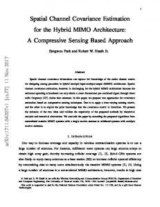
Figure 1: Geometry setting of the test mixture. Source variance estimation Blind

Oracle

October 18-21, 2009, New Paltz, NY

Covariance model

Rank

SDR

SIR

ISR

anechoic convolutive direct+diffuse unconstrained anechoic convolutive direct+diffuse unconstrained

1 1 2 2 1 1 2 2

0.9 4.0 3.1 5.8 0.4 4.2 10.2 10.9

1.7 6.4 6.1 10.3 4.4 10.2 17.3 17.9

4.8 8.5 7.3 10.5 7.5 6.2 11.7 12.5

6. REFERENCES [1] O. Yılmaz and S. Rickard, “Blind separation of speech mixtures via time-frequency masking,” IEEE Trans. on Signal Processing, vol. 52, no. 7, pp. 1830–1847, July 2004. [2] S. Winter, W. Kellermann, H. Sawada, and S. Makino, “MAP-based underdetermined blind source separation of convolutive mixtures by hierarchical clustering and ℓ1 -norm minimization,” EURASIP Journal on Advances in Signal Processing, vol. 2007, 2007, article ID 24717.

Table 1: Average source separation performance.

[3] C. F´evotte and J.-F. Cardoso, “Maximum likelihood approach for blind audio source separation using timefrequency Gaussian models,” in Proc. 2005 IEEE Workshop on Applications of Signal Processing to Audio and Acoustics (WASPAA), 2005, pp. 78–81.

impulse responses simulated via the source image method so that the geometry setting, i.e. showned in Fig 1, is known exactly. The STFT was computed with a sine window of length 1024 (64 ms). The bi-dimensional window 𝑤 defining time-frequency neighborhoods in (11) was chosen as the outer product of two Hanning windows with length of 3 [4]. Computation time was on the order of 5 min per model in the semi-blind case using Matlab on a 2.4 GHz computer. Separation performance was evaluated using the signal-to-distortion ratio (SDR), signal-to-interference ratio (SIR) and source image-to-spatial distortion ratio (ISR) criteria in [9], averaged over all sources. The results are shown in Table 1. The rank-1 anechoic model has lowest performance because it only accounts for the direct path. In a semi-blind context, the full-rank direct+diffuse model results in a SDR decrease of 1 dB compared to the rank-1 convolutive model. This decrease appears surprisingly small when considering the fact that the former involves 8 spatial parameters (6 dis2 tances 𝑟𝑖𝑗 , plus 𝜎rev and 𝑑) instead of 3078 parameters (6 mixing coefficients per frequency bin) for the latter. The full-rank unconstrained model improves the SDR by 2 dB and 2.5 dB when compared to the rank-1 convolutive model and binary masking method respectively. In an oracle context, full-rank models clearly outperform rank-1 models by 6 dB or more regarding all criteria. Also, the performance of the full-rank direct+diffuse model is very close to that of the unconstrained model.

[4] E. Vincent, S. Arberet, and R. Gribonval, “Underdetermined instantaneous audio source separation via local Gaussian modeling,” in Proc. Int. Conf. on Independent Component Analysis and Signal Separation (ICA), 2009, pp. 775–782. [5] A. Ozerov and C. F´evotte, “Multichannel nonnegative matrix factorization in convolutive mixtures. With application to blind audio source separation.” in Proc. Int. Conf. on Acoustics, Speech and Signal Processing (ICASSP), April 2009. [6] J. F. Cardoso and M. Martin, “A flexible component model for precision ICA,” in Proc. Int. Conf. on Independent Component Analysis and Signal Separation (ICA), 2007, pp. 1–8. [7] T. Gustafsson, B. D. Rao, and M. Trivedi, “Source localization in reverberant environments: Modeling and statistical analysis,” IEEE Trans. on Speech and Audio Processing, vol. 11, pp. 791–803, Nov 2003. [8] H. Kuttruff, Room Acoustics, 4th ed., New York, 2000. [9] E. Vincent, H. Sawada, P. Bofill, S. Makino, and J. Rosca, “First stereo audio source separation evaluation campaign: data, algorithms and results,” in Proc. Int. Conf. on Independent Component Analysis and Signal Separation (ICA), 2007, pp. 552–559.

5. CONCLUSION

[10] A. Yeredor, “On using exact joint diagonalization for noniterative approximate joint diagonalization,” IEEE Signal Processing Letters, vol. 12, no. 9, pp. 645–648, Sep 2005.

In this paper, we proposed to model the spatial properties of sound sources by full-rank spatial covariance matrices and studied a pos-

132