Spatial Extent of Random Laser Modes Karen L. van der Molen,1, ∗ R. Willem Tjerkstra,1 Allard P. Mosk,1 and Ad Lagendijk2
arXiv:cond-mat/0612328v2 [cond-mat.dis-nn] 27 Feb 2007
1
Complex Photonic Systems, MESA+ Institute for Nanotechnology and Department of Science and Technology University of Twente, P.O. Box 217, 7500 AE Enschede, The Netherlands. 2 FOM Institute for Atomic and Molecular Physics (AMOLF), Kruislaan 407, 1098 SJ Amsterdam, The Netherlands (Dated: February 5, 2008) We have experimentally studied the distribution of the spatial extent of modes, and the crossover from essentially single-mode to distinctly multi-mode behavior inside a porous gallium phosphide random laser. This system serves as a paragon for random lasers due to its exemplary high index contrast. In the multi-mode regime we observed mode competition. We have measured the distribution of spectral mode spacings in our emission spectra, and found level repulsion that is well described by the Gaussian orthogonal ensemble of random-matrix theory. PACS numbers: 42.55.Zz, 42.25.Dd, 78.55.Cr
Random lasers, in which gain is combined with multiple scattering of light [1, 2], are the subject of active research [3, 4, 5, 6]. The discovery of intriguingly narrow spectral emission peaks (spikes) in certain random lasers by Cao et al. [7] has given an enormous boost to this field of research [8, 9, 10, 11, 12, 13, 14]. In the past few years a debate on the origin of these spikes has started [14, 15, 16, 17, 18, 19, 20, 21, 22]. On one hand Cao et al. [16], as well as Sebbah and Vanneste [15] and Apalkov et al. [17], attribute the spikes to local cavities (local modes, LM) for light, which are formed by multiple scattering. On the other hand Mujumdar et al. [14], as well as Pinheiro and Sampaio [21], attribute the spikes to single spontaneous emission events that, by chance, follow very long light paths (open modes, OM) in the sample and hence pick up a very large gain. The LM and the OM model we cite represent divergent answers to the question what the spatial extent is of the modes responsible for the spikes. The spatial extent of the modes is a crucial factor for the fundamental behavior of a random laser. If the spatial extent of the modes is small, and the modes do not spatially overlap, the laser effectively consists of a collection of single-mode lasers. In contrast, spatially overlapping modes inside the random laser lead to distinctly multi-mode behavior, such as mode competition [23]. In this Letter, we present the first systematic study of the spatial extent of the modes of a random laser, and show the crossover from essentially single-mode to multimode behavior in a new type of random laser: single crystal porous gallium phosphide [24], filled with liquid dye solution. Among other conclusions, our results indicate that the LM model describes the physics of our random laser better than the OM model, but the LM model needs more sophistication. Our random laser consists of porous gallium phosphide obtained by anodic etching (porosity, 45% air; thickness, > 46µm), of which the pores are filled with a 10 mmol/l solution of rhodamine 640 perchlorate in
methanol (pump absorption length, 22 µm; minimal gain length, 12 µm [25]). This random laser combines three characteristics which sets it apart from other random lasers. Firstly, the position of the scatterers is rigidly fixed. Secondly, the efficient laser dye rhodamine 640 ensures high gain. Finally, the contrast of the refractive indices in the sample is the highest ever reported for random lasers: n = 1.33 for methanol and 3.4 for gallium phosphide. The method of fabrication of the porous gallium phosphide is slightly modified from the method described earlier [26, 27]. We used n-GaP with a dopant density of 2·1017 /cm2 , obtained from Marketech. To make porous GaP without a non-porous top layer, the GaP is anodically etched in 0.5 M H2 SO4 . In the first step, the potential is set to 22.5 V until 5 C/cm2 has passed through the sample. In the next step, the potential is switched to 30 V for 10 minutes. In the third step, the potential is switched back to 22.5 V. The GaP is etched until 60 C/cm2 has passed through the sample. After finishing the etching process, the first layer can easily be removed, leaving porous GaP. The transport mean free path ℓ of our samples filled with pure methanol is measured with an enhancedbackscatter-cone experiment [28] and is 0.6 ± 0.3 µm at λ = 633 nm (k0 ℓ = 6.4 ± 2.8, with k0 the vacuum wavenumber, neff = 2.1 ± 0.4). The sample holder has a sapphire window with a thickness of 3 mm. The random laser sample is lightly pushed onto the window with a spring. A detailed calculation shows that the emitted laser-light is generated inside the pores of the gallium phosphide, and cannot be generated by the dye between the window and the sample. The sample holder can be translated in one direction (parallel to the surface of the sample) with a total displacement of 12 mm by means of a stepper motor. The pump source is a tunable optical parametric oscillator (Coherent Infinity 40-100/XPO). The pump pulse, at a wavelength of 567 nm, has a duration of 3 ns and a rep rate of 50 Hz. The wavelength of the pump source is chosen to avoid dam-
Spectral pulse energy (pJ/nm)
2
2000
1500
1000
500
0 604
605
606
607
608
Wavelength (nm)
FIG. 1: (Color) Two emission spectra of the random laser collected at the same spot on the sample. One spectrum (black) before, and one (red) after shifting the sample by 37 µm and back. Apparently, the frequencies of the modes are fully determined by the realization of the disorder.
age through absorption of light by gallium phosphide, and to obtain high enough gain of the dye. The pump light is spatially filtered, and focused with a microscope objective (numerical aperture, 0.55) onto the sample (focus area, 3 ± 1 µm2 ). The pump energy on the sample was at maximum 0.32 µJ/pulse. Emission light of the random laser is collected through the microscope objective, dispersed by a spectrometer (resolution, 1 cm−1 ) and detected by an electron-multiplier charged-coupled device (C9100-02, Hamamatsu) [35]. The responsivity of the system was calibrated with an Ophir power meter (PD300-3W) and a HeNe-laser. All measurements presented in this Letter are measured at an input energy of twice the threshold input energy, except Fig. 3. This threshold is defined as the collapse of full width at half maximum (FWHM) of the emitted spectrum [2]. The FWHM of the spectrum far above threshold is 13 times narrower than the FWHM of the emitted spectrum below threshold. To discriminate between current models, and possibly stimulate new theoretical approaches, we want to investigate whether mode frequencies are completely determined by the realization of disorder inside the random laser. In contrast to the frequencies of the modes, we expect that in all cases the peak intensities will depend on the pump energy; as we have pulse-to-pulse fluctuations of our pump source, we expect a different overall scale factor for our peak intensities for every shot. We collected several spectra above threshold at a single position on the sample. In between measurements, the sample was translated 37 µm and back. Two of the resulting spectra are shown in Fig. 1 [36]. The spectral positions of the modes reproduce, proving that mode frequencies are completely determined by the realization of disorder, and not selected by spontaneous emission events. In addition to the expected overall scale factor the peak intensities above threshold differed individually from shot-to-shot, as is shown in Fig. 1. To investigate the origin of this height-distribution variation, we
FIG. 2: (Color) One of the 50 single-shot-emission spectrum of our random laser system collected at one position of the sample. The symbols near the peaks correspond to the pulse energy of those peaks in Fig. 3.
looked at the emission spectrum of the random laser at a single position for different pump energies. We took 50 single shot measurements, and used the measured pulseto-pulse variation of the pump source to obtain a range of pump energies. Above threshold we observed a linear relation between the total energy of the emitted light and the pump energy. A typical emission spectrum is shown in Fig. 2. We determined the energies in the observed 4 narrow peaks in the emission spectrum (integration of spectrum over 0.576 nm). In Fig. 3 we plotted these energies versus the total pulse energy of the emitted light. When the total emitted pulse energy increases above a threshold of 50 pJ, we observed that a single mode starts to lase (star symbol). In this regime, the random laser can be described as a single-mode laser. We found a decrease of the spectral width of this single mode for increasing pulse energy in the mode, in correspondence with the well-known Schawlow-Townes behavior [29]. At higher emitted pulse energies (125 to 150 pJ) two more modes of the random laser start to lase, whereas the energy in the first mode does not increase anymore. This leveling-off is a clear sign that the modes are competing for the available energy, and thus are overlapping in space. This spatial mode competition causing the heightdistribution variation is not related to the frequencies of the modes. To directly observe the spatial extent of the modes inside the random laser, we measured emission spectra while pumping at different positions of the sample. In contrast, using speckle correlation techniques it is possible to determine the spatial extent of the secondary light source on the surface, originating from the scattered light [16]. In our experiment the sample was horizontally translated with steps of 506 ± 4 nm, and for every position of the sample 50 single-shot-emission spectra were collected. We displaced the sample 20 µm in total, which is 10 times the diameter of the pump spot. In Fig. 4 zoom-in of collected spectra at 5 consecutive positions are shown [37]. Figure 4 is a visualization of a typical evolution of a peak in the emission spectrum as the po-
3
FIG. 3: (Color) Pulse energy in 4 modes [see for single-shot emission spectrum Fig. 2] versus the total emitted pulse energy of the collected light for 50 single-shot spectra. The measured errors are smaller than the symbol size. The solid line is a guide to the eye for the star symbols. Clearly, one mode starts to lase (star symbol), before the other modes begin to lase at higher pump energies.
Spectral pulse energy (pJ/nm)
1000
Displacement: 0.0 mm
0 1000
0.5 mm
0 1000
FIG. 5: Measured distribution of the spatial size of the modes determined with a displacement measurement. The dotted line is a marker for the diameter of the focus of the pump source on the sample.
1.0 mm
0 1000
1.5 mm
0 1000
2.0 mm
0 605.0
605.2
605.4
605.6
605.8
606.0
Wavelength (nm) FIG. 4: Enlargement of a part of the emission spectra where a peak is visible. Between consecutive spectra, the sample is translated by 506 nm.
sition of the sample is changed. First a peak becomes visible. Additional displacement of the sample leads to an intensity going through a maximum. The increase and decrease of intensity corresponds to the overlap between the gain region and the mode. The spatial extent of mode is defined by the difference in sample position where the mode rises above noise level and the position where the mode falls below the noise level (noise level is 5%). In the specific case of Fig. 4 the spatial extent is 2.5 ± 0.5 µm. In Fig. 5 the distribution of the spatial extent of all the modes is plotted, together with a marker of the diameter of the focus of the pump source on the sample. Almost 80% of the modes have a spatial extent smaller
than the diameter of the spot size of the focus (2 µm). The other 20% of the modes are larger than the diameter of the spot size of the focus. For the LM (OM) model, we would expect all modes to have a spatial extent much smaller (larger) than the focus diameter of the pump spot. Apparently, our measured distribution disagrees with the expectation of either of the two models. The selection criterium for a mode to lase is its dwell time [30]. Our observed limited spatial extent of lasing modes suggests that modes with long dwell times have small spatial extent. This connection has never been put forward before, and may be unique to three dimensional strongly scattering media [13]. We will now focus on the statistics of spectral spacings of the modes. For 11 spectra taken at widely spaced positions, we determined the spectral spacing between two adjacent peaks. These 11 spectra are statistically independent but equivalent. The only difference is the position on the sample where the data was collected. Therefore we combine the 41 spectral spacings of these 11 spectra in one distribution. In Fig. 6 we plot this distribution of the spectral mode spacing. Surprisingly, our observations show that the statistics are determined by level repulsion, in complete analogy to level repulsion in quantum mechanics [31, 32]. A first experimental indication of spectral level repulsion was shown by Cao et al. [33]. To describe level repulsion quantitatively we compare our observed statistics of the spectral mode spacings to the results of random-matrix theory. Although random matrix theory does not necessarily apply here, it does describe avoided crossings. The distribution of mode spacings according to the Gaussian orthogonal ensemble
4
Electronic address:
[email protected] [1] V. S. Letokhov, Sov. Phys. JETP 26, 835 (1968). [2] N. M. Lawandy et al., Nature (London) 368, 436 (1994). [3] A. C. Vutha, S. K. Tiwari, and R. K. Thareja, J. Appl. Phys. 99, 123509 (2006). [4] D. Sharma, H. Ramachandran, and N. Kumar, Opt. Lett. 31, 1806 (2006). [5] M. Noginov et al., J. of Opt. A 8, s285 (2006). [6] A. Rose et al., Nature (London) 434, 876 (2005). [7] H. Cao et al., Appl. Phys. Lett. 73, 3656 (1998). [8] H. Cao, J. Phys. A: Math. Gen. 38, 10497 (2005). [9] S. F. Yu et al., Appl. Phys. Lett. 84, 3241 (2004). [10] S. V. Frolov et al., Opt. Commun. 162, 241 (1999). [11] R. C. Polson and Z. V. Vardeny, Phys. Rev. B 71, 045205 (2005). [12] V. Milner and A. Z. Genack, Phys. Rev. Lett. 94, 073901 (2005). [13] M. A. Noginov, J. Novak, and S. Williams, Phys. Rev. A 70, 063810 (2004). [14] S. Mujumdar et al., Phys. Rev. Lett. 93, 053903 (2004). [15] P. Sebbah and C. Vanneste, Phys. Rev. B 66, 144202 (2002). [16] H. Cao et al., Phys. Rev. E 66, 025601(R) (2002). [17] V. M. Apalkov, M. E. Raikh, and B. Shapiro, Phys. Rev. Lett. 89, 016802 (2002). [18] V. M. Markushev et al., Laser Physics 15, 1611 (2005). [19] L. I. Deych, Phys. Rev. Lett. 95, 043902 (2005). [20] L. Angelani et al., Phys. Rev. Lett. 96, 065702 (2006). [21] F. A. Pinheiro and L. C. Sampaio, Phys. Rev. A 73, 013826 (2006). [22] A. D. Stone and H. E. Tureci, Photonic Metamaterials: From Random to Periodic on CD-ROM (The Optical Society of America, Washington, DC, 2006), Vol. WC2. [23] R. V. Ambartsumyan et al., Prog. in Quant. Electron. 1, 107 (1970). [24] F. J. P. Schuurmans et al., Science 284, 141 (1999). [25] W. B¨ aumler et al., Meas. Sci. Technol. 3, 384 (1992). [26] B. H. Ern´e, D. Vanmaekelbergh, and J. J. Kelly, J. Electrochem. Soc. 143, 305 (1996). [27] R. W. Tjerkstra et al., Electrochemical and Solid-State Letters 5, G32 (2002). [28] M. P. van Albada and A. Lagendijk, Phys. Rev. Lett. 55, 2692 (1985); P. E. Wolf and G. Maret, ibid. 55, 2696 (1985). [29] A. L. Schawlow and C. H. Townes, Phys. Rev. 112, 1940 (1958). [30] K. L. van der Molen, A. P. Mosk, and A. Lagendijk, Phys. Rev. A 74, 053808 (2006). [31] C. W. J. Beenakker, Rev. Mod. Phys. 69, 731 (1997). [32] M. Patra, Ph.D. thesis, University of Leiden, 2000. [33] H. Cao et al., Phys. Rev. B 67, 161101 (2003). [34] T. Guhr, A. M¨ uller-Groeling, and H. A. Weidenm¨ uller, Physics Reports 299, 189 (1998). [35] The slit of the spectrometer was set to 55 ± 15 µm. A change in the incident angle of light caused the spectral position to shift, shown spectra were corrected. [36] Hysteresis of the stepper motor causes the sample not to return exactly to the same position (systematic error 0.04 µm). The red spectrum is shifted accordingly by 0.07 nm. [37] Spectra of Fig. 4 are shifted with respect to the top one by 0.154 nm, 0.211 nm, 0.274 nm, 0.288 nm, respectively. ∗
FIG. 6: Measured distribution of the spectral mode spacing for 11 emission spectra. The solid line is a fit of Wigner’s surmise (1). The fit parameter is the mean mode spacing ∆, we find ∆ = 16.2 cm−1 .
(GOE) is given by Wigner’s surmise [34] P (x) = Cxe−πx
2
/(4∆2 )
,
(1)
where P is the distribution of the mode spacing x of the modes, ∆ the mean mode spacing, and C a scaling factor. In Fig. 6 we plot the fit of Eq. (1) (black line), with a mean GOE mode spacing ∆ of 16.2 ± 0.9 cm−1 . When considering all modes in a multiple scattering system the level statistics is known to be Poissonian (exponential) [34]. In this experiment we only observe those modes that lase and they show level repulsion. Apparently, the selection mechanism for random lasing causes the level statistics to change from Poissonian statistics to level repulsion. We have performed a systematic study of random lasing in porous gallium phosphide. The frequencies of the modes in our sample are determined by the realization of disorder. We have observed a variation in the height distribution, and attributed this variation to spatial mode overlap and gain competition. The distribution of the spectral mode spacings shows clear level repulsion and can be described with the Gaussian orthogonal ensemble. In addition the (small) spatial extent of lasing modes was observed. We hope that our observations stimulate more theoretical work. The authors thank Boris Bret for preliminary measurements, and Paolo Scalia and Sanli Faez for their help with the characterization measurements. We acknowledge discussions with Carlo Beenakker on the possible origins of level repulsion in random lasers. This work is part of the research program of the Stichting voor Fundamenteel Onderzoek der Materie (FOM), which is financially supported by the Nederlandse Organisatie voor Wetenschappelijk Onderzoek (NWO).
5