The theory of random laser systems

Iowa State University

Digital Repository @ Iowa State University Retrospective Theses and Dissertations

2001

The theory of random laser systems Xunya Jiang Iowa State University

Follow this and additional works at: http://lib.dr.iastate.edu/rtd Part of the Condensed Matter Physics Commons, and the Optics Commons Recommended Citation Jiang, Xunya, "The theory of random laser systems " (2001). Retrospective Theses and Dissertations. Paper 1050.

This Dissertation is brought to you for free and open access by Digital Repository @ Iowa State University. It has been accepted for inclusion in Retrospective Theses and Dissertations by an authorized administrator of Digital Repository @ Iowa State University. For more information, please contact [email protected].

INFORMATION TO USERS

This manuscript has been reproduced from the microfilm master. UMI fiims the text directly from the original or copy submitted. Thus, some thesis and dissertation copies are in typewriter face, while others may be from any type of computer printer.

The quality of this reproduction is dependent upon the quality of the copy submitted. Broken or indistinct print, colored or poor quality illustrations and photographs, print bleedthrough, substandard margins, and improper alignment can adversely affect reproduction..

In the unlikely event that the author did not send UMI a complete manuscript and there are missing pages, these will be noted.

Also, if unauthorized

copyright material had to be removed, a note will indicate the deletion.

Oversize materials (e.g., maps, drawings, charts) are reproduced by sectioning the original, beginning at the upper left-hand corner and continuing from left to right in equal sections with small overlaps.

Photographs included in the original manuscript have been reproduced xerographically in this copy.

Higher quality 6" x 9" black and white

photographic prints are available for any photographs or illustrations appearing in this copy for an additional charge. Contact UMI directly to order.

ProQuest Information and Learning 300 North Zeeb Road, Ann Arbor, Ml 48106-1346 USA 800-521-0600

The theory of random laser systems by Xunya Jiang

A dissertation submitted to the graduate faculty in partial fulfillment of the requirements for the degree of DOCTOR OF PHILOSOPHY

Major: Condensed Matter Physics Major Professor: Costas M. Soukoulis

Iowa State University Ames, Iowa 2001

UMI Number: 3016715

®

UMI

UMI Microform 3016715 Copyright 2001 by Bell & Howell Information and Learning Company. All rights reserved. This microform edition is protected against unauthorized copying under Title 17, United States Code.

Bell & Howell Information and Learning Company 300 North Zeeb Road P.O. Box 1346 Ann Arbor, Ml 48106-1346

1

The theory of random laser systems Xunya Jiang Major Professor: Costas M. Soukoulis Iowa State University Random laser systems are studied not only for their interesting physical properties, but also for their importance in technological applications. Their basic property is that the lasing phenomenon can appear in the random systems with gain. Randomness, which was thought to be detrimental to the lasing feedback mechanism, is a essential element in such lasing systems. The theoretical research of the random laser systems is based on the localization theory and laser physics. In this dissertation we study the random laser systems in several aspects. First we will study the transmission and the reflection of the systems by the transfer matrix method. The analytical formula of the critical length or critical gain of random laser systems will be derived by the comparison between Lamb's theory and Letokhov's theory. Second, with the theoretical analysis and the numerical results, we will point out that the previous time-independent methods, which were widely used in the research of the random laser systems, will give us unphysical results when the gain is over the threshold of the system. Then, we will construct a model, with the FDTD method and the semiclassical laser physics, to study the new experimental results. This model can not only explain the multi-peak and anisotropic spectra of experiments, but also predict the lasing-mode number saturation in random laser systems. With this model, both of the time-evolving process and the final-stable solution of the random lasing modes can be studied. Finally, we will theoretically and numerically study the properties of the random lasing modes. We will derive the eigenequation and the magnitude equation of the modes to support our numerical results which will show that the wavefunctions of modes retain almost same in the lasing process, and the threshold of a mode can be predicted by the quality factor of the mode and the gain profile of amplifying medium. We suppose that these properties of the random lasing modes will be a new path for observing localization.

ii

Graduate College Iowa State University

This is to certify that the Doctoral dissertation of Xunya Jiang has met the dissertation requirements of Iowa State University

Signature was redacted for privacy.

Signature was redacted for privacy.

For the Major Program Signature was redacted for privacy.

For the Graduate College

iii

TABLE OF CONTENTS

CHAPTER 1. GENERAL INTRODUCTION History and Steps of Development

1 2

History of localization theories

2

History of laser physics

3

Development of the random laser theories

5

Theoretical Background of Wave Localization Physical picture Differences between classical and quantum waves Theoretical Background of Laser Physics

7 7 10 12

What is a laser?

12

Mechanism of lasing process

12

Coherent properties

14

Theoretical Formulation and Numerical Methods

15

Theoretical formulation of gain medium

15

Formula of transfer matrix method

18

Formula of FDTD calculation

18

Dissertation Organization

19

Bibliography

21

CHAPTER 2. TRANSMISSION AND REFLECTION STUDIES OF PE­ RIODIC AND RANDOM SYSTEMS WITH GAIN

25

Abstract

25

Introduction

25

iv

Theoretical Models

28

Many-layered model of classical wave

28

Electronic tight-binding model

29

Periodic Systems Classical many-layered model Electronic tight-binding model

30 30 32

Random Systems

32

Probability Distribution of Reflection Coefficient

38

Conclusion

39

Acknowledgment

40

Bibliography

40

CHAPTER 3.

IS THERE A SYMMETRY BETWEEN ABSORPTION

AND AMPLIFICATION IN DISORDERED MEDIA?

50

Abstract

50

Introduction

50

Theoretical Model and Derivation

52

Numerical Results of FDTD Model

54

Conclusion

56

Bibliography

57

CHAPTER 4. TIME DEPENDENT THEORY FOR RANDOM LASERS .

62

Abstract

62

Introduction

62

FDTD model

64

Numerical Results and Theoretical Discussion

67

Conclusion

69

Bibliography

69

CHAPTER 5. THEORY AND SIMULATIONS OF RANDOM LASERS . . Abstract

74 74

V

Introduction

74

Theoretical Model

77

Localized Modes of Random Laser Systems

80

The Saturated Number of Lasing Modes

82

Dynamic Processes

84

Conclusions

86

Bibliography

87

CHAPTER 6. LOCALIZED RANDOM LASING MODES AND A NEW PATH FOR OBSERVING LOCALIZATION

98

Abstract

98

Introduction

98

Numerical results

100

Theoretical results and discussion

102

Conclusion

104

Bibliography

105

CHAPTER 7. GENERAL CONCLUSIONS

110

1

CHAPTER 1. GENERAL INTRODUCTION

My graduate work focuses on the theory of random laser systems which is a very new direction in condensed matter physics. The topics in random laser systems are about the electromagnetic (EM) wave propagation in random and amplifying media. The development of this direction is based on the background of the two very important branches of modern condensed matter physics: one is localization of waves, and the other is laser physics. Both were started in the sixties and are still under intensive study. Localization theories give us basic physical understanding of how waves propagate in random media, while the laser theories tell us how EM waves interact with gain media in cavities. Random laser systems are studied not only for their interesting physical properties, but also for their importance in technological applications. Fundamentally, the study of random laser systems helps us understand how the localization effects interplay with coherent amplifi­ cation and how a random lasing mode evolves in the lasing process. These systems are a new tool to study the localization effects of the random systems and the chemical properties of the gain medium. The promising industrial uses of random laser systems are cheap and efficient sources of light, including micro-lasers, paint, pixels, photonic marking for identification pur­ poses (photonic codes, search-and-rescue missions, military applications, marking of hazardous materials) and photo-dynamics therapy. Next, I review the history of this direction and introduce background knowledge of lo­ calization of waves and laser physics respectively. Then I introduce theoretical formulation and numerical methods which we will encounter many times in this thesis. Finally, I give the organization of this dissertation.

2

History and Steps of Development History of localization theories Wave (classical wave or quantum particle) propagation in random medium has been studied for centuries [1]. In the 19th century and the beginning of the 20th century, Brownian motion was studied by Langevin and Einstein [2]. The diffusion equation was obtained. With the diffusion coefficient, the random walk of classical particles could be quantitatively studied. The classical non-equilibrium transport problem was studied by Boltzmann who developed the famous Boltzmann equation [2]. The Boltzmann equation can also be derived by quantum theory with the ladder diagram approximation [3]. So Boltzmann's equation is very important and correct most of the time for studying transport properties. It's even useful for quantum particles such as in calculations of the conductivity in condensed matter physics. But in the Boltzmann equation, the particle is a classical one, so when quantum effects are important, we need to reconsider the Boltzmann formulation. The reformulation of the Boltzmann theory was started by Anderson in 1958, when he first introduced the localization [4] referring to a dramatic change in the propagation of an electron when it is subjected to a spatially random potential. Problems in which the localization effects are important can be judged by the IoffeRegel criterion 2irl/\ % 1 [5], where I is the mean free path, and A is the wavelength in the medium. In 1972, Edwards and Thouless [6] proposed a scaling criterion for localization based upon the sensitivity of electronic wavefunctions to the boundary of the sample, and this was the beginning of the scaling theory of localization study. In 1980 Anderson, Thouless, Abrahams, and Fischer [7] developed the scaling theory of localization. The scaling theory suggests us that all the states are localized if the dimension of the system is less than or equal to two. For a 3D system, waves are only localized for strong enough randomness. Several approaches can be used to describe the phenomenon of localization in a disordered medium. One method is to look at the transport properties of the electron. In this picture localization is concerned with the vanishing (zero) of the diffusion coefficient. Another method is to look at the eigenstates of the electron in a random system. If every eigenstate in a certain

3

energy range decays exponentially from a spatial center, we call the state a localized state. So the localized states, unlike extended states, are not sensitive to the change of the boundary conditions. This is the reason for Thouless's scaling argument. The transition of the states from extended to localized is called localization transition or Anderson transition. The energy which separates the extended states from the localized states is called mobility edge. In 1984, localization was first introduced to classical waves (electromagnetic waves) by S. John [8, 9] . At the same time, coherent backscattering as the signature of localization was suggested by Bergmann [10]. This clear physical picture tells us that the wave interfering effects are the cause of localization. The constructive interference of two time-reversed paths will make the quantum waves (quantum particles) and classical waves prefer to stay at their original place. In other words, these waves are lazier and more difficult to transport than the classical particles. There are two necessary conditions for coherent backscattering, the first is that waves keep their phase memory in the scattering process, and the second is the time-reversal symmetry exists in the scattering process. In 1984 Economou, Soukoulis, and Zdetsis [11] obtained the mobility edge trajectory for the propagation of electrons in 3D by the coherent potential approximation (CPA) method. In addition, they [12] mapped the electronic problems to the classical case and make prediction for the possible optimum conditions of observing localization of classical waves. John [13] also introduced the photonic band gap (PBG) material [1] as a strong candidate to realize the localization of light in 1986. But, so far the localization of classical waves in the 3D systems is still not resolved Itiggelen, Iwiersmanature. History of laser physics For laser physics, the development of theory and applications has continued since 1960 [16, 17, 18], and it has evolved into an independent field. In 1917, Einstein [19] postulated the process of stimulated emission, thus laying the foundation for the invention and the develop­ ment of lasers. In 1960, the development of laser engineering and laser physics was pushed suddenly by the operation of the first ruby laser [20]. In 1964, Lamb [21] proposed a theoretical

4

description for the operation of a multimode laser oscillator, based on a classical description of the electromagnetic field in terms of high-Q modes, and a quantum mechanical description of the amplifying medium. Lamb's theory developed in the sixties is the basic theory for under­ standing the detailed behaviors of laser systems, such as mode competition, dynamic processes etc. More complex theories have been constructed since then, based on a better understanding of quantum electromagnetic field theory and the interaction between the atomic field and the electromagnetic field. Full quantum field theories evolved during the latter half of the 1960s. But in full quantum field theories, the description of the thermal reservoir and the process of excitation is difficult. Three types of theory were introduced. In 1966, H. Haken [22] introduced the classical Langevin equation into the Heisenberg equation and constructed a new method to study laser systems. The second one was developed by Scully and Lamb [23] in 1968 who used density matrix to describe the system and treated thermal reservoir as a perturbation. The third method was introduced by Risken [24] and Haken [25] in 1965 based on the Fokker-PIanck equation. After more understanding of quantum mechanics in the seventies and eighties, many new concepts such as coherent states, squeezed states, EPR paradox, geometry (Berry) phases, quantum computation and quantum chaos, etc., were introduced into laser physics [26]. So far laser physics continues to develop. But for our studies of the random laser system, we will only use the semi-classical Lamb's theory [17, 21]. Distributed-feedback laser [18], in which the reflection feedback takes place not only at the end reflectors but continuously throughout the length of the resonator, was first constructed in 1972 [27]. Actually in most cases, distributed-feedback lasers are the ID photonic band gap (PBG) systems made of amplifying media. PBG systems are another promising development in modern condensed matter physics and optical physics. The topic of 3D PBG systems was first introduced in 1987 by S. John [13] and E. Yablonovitch [28] independently for the purposes of the classical wave localization and the spontaneous emission suppression, respectively. The first prediction of a structure that has a true 3D PBG gap was done by Ho, Chan and Soukoulis [29] in 1990. Actually, random lasers are one kind of distributed-feedback lasers. One way to

5

make random laser systems is to introduce randomness into a common distributed feedback laser systems. Development of the random laser theories Random laser systems were first theoretically proposed by Letokhov [30] in 1968 using the diffusion equation. However, it was believed for a long time that the scattering in random systems is detrimental for the lasing process, because the scattering reduces the coherent feedback of light in common laser systems. Thus, random laser systems had been relatively unnoticed for about 35 years, until experiments and explanation by Lawandy's group in 1994 [31]. Lawandy's group observed a narrowing of the spontaneous emission spectrum when the scatterer's density was over a certain value. They named this phenomenon laser-like emission and reminded us of the original work of Letokhov. This work stimulated experimentalists [32, 33] and theorists [34, 35, 36, 37, 38, 39, 40] to work in this area and since then experiments and theories are developing at almost the same speed. Many experiments were carried out that showed a drastic spectral narrowing [32] and a narrowing of the coherent backscattering peak [33]. In 1995, Zyuzin [35] theoretically got a sharp and higher coherent backscattering peak by a path integral method in a random amplifying medium. So we can see that the localization effects (coherent backscattering) are important in random laser systems. John and Pang [36] in 1996 developed a theoretical model by combining the electron population equations on energy levels with the diffusion equation and obtained similar spectra narrowing. Genack's group [37] based on a random walk model and a frequency-dependent gain profile also obtained spectra narrowing in 1997. The time-independent transfer matrix method was used by Zhang [38] on a random laser system in 1995. Zhang extended Letokhov's theory by introducing the localization length into a ID random laser system and calculated the mean threshold length of systems from the localization length and the gain length. In 1999, Jiang and Soukoulis [43] compared the Letokhov theory and the Lamb theory in laser physics and extended this relation to systems with a periodic background. Between 1995 and 2000 many papers [38, 39, 40, 41, 42] used the

6

time — independent transfer matrix method and the time — independent invariant embedding method to study nandom laser systems. They obtained an exponential decay of the transmission and probability distribution of the reflection in half-infinite long random amplifying systems. However, in 2000 Jiang, Li and Soukoulis [44] pointed out that all time-independent theories give unphysical reesults (such as an exponential decay of the transmission and finite reflection in a very long sys~tem), if the length or the gain of system is over the lasing threshold. But, the transfer matrix m ethod is still a useful numerical method to obtain the threshold and the modes of random amplifying systems. We also used [44] a finite-difference

time-domain (FDTD)

method to demonstrate that the numerical results are totally different for time-dependent theories and time-independent theories. In 1999, Cao's group [45] at Northwestern University observed new phenomena in random laser systems. Vaerdeny's group [46] at University of Utah found similar phenomena in 2000. Both groups found multi-lasing-peak and anisotropic properties in the output spectrum of random laser systtems. Such un predicted phenomena set a new challenge to theoretical re­ searchers. These lasing peaks were supposed to originate from the lasing modes in the random systems. But, wiry weren't these modes predicted from earlier theoretical work? What are the properties of thes#e modes? How can we theoretically study these modes? The reason w_h.y the lasing modes in random laser systems are not predicted is that all previous theoretical work is based on mean field methods . Actually, we can obtain these modes by the time-independent transfer matrix method, but theorists used the average of many random configurations to explain the experimental results. However, all time-independent methods have a \rital weakness because they can not explain over-threshold pumping cases as we pointed out [4-4]. So what do we= need to construct a model to explain such phenomena? First, the theoretical method should be time-dependent, such as the FDTD method. Second, we must use a certain random configuration and wave equations to get the modes. Third, we need the amplifying mechanism in oui model. Of course, if the theory of the amplifying mechanism is realistic, the model is bett-er and gives us more detailed information about the system. Of course, to

7

implement such a scheme, longer computing time is needed. In 2000, Jiang and Soukoulis [47] introduced a scheme for the random laser systems which includes the FDTD calculation, time-dependent Maxwell equations, a certain random configuration of the system, and semiclassical theory of the gain medium. From this scheme, we find that the multi-Iasing peaks are indeed from the lasing modes inside the system. We also predicted the mode repulsion properties in random laser systems and the saturation of the number of lasing mode. These results are confirmed by experiments of Cao's group [48]. We also use this model to study the properties of localized modes [49]. It is found that the wavefunctions of the lasing modes stay almost the same before and after we introduce gain into the random systems. These numerical results can be explained by Lamb's theory of laser physics. We also find that the lasing thresholds of these modes depend on the quality factor Q of the modes and on the gain profile. We can predict which mode will lase first if we have this information. These properties give us a new path to study the localization of classical waves in random systems, such as finding the mobility edge and studying the localized states inside the random systems. So, we can see that the knowledge of the random laser systems will help us to study the properties of localization of waves. We also use the model to study the dynamic process [48] of random laser systems. For this topic, we collaborate with Cao's experimental group from Northwestern University. With pulsepumping cases, both theoretical and experimental results show that the different modes lase at different time and last for different time lengths. We also find for the first time relaxation oscillation of modes in random lasers. Theoretically, we can explain the oscillation by the interaction between the lasing field and the electron population on different energy levels.

Theoretical Background of Wave Localization Physical picture Localization was started at the study of quantum waves (electrons) in random potentials, but later it was found that the electron transport in disordered potentials and the photon transport in random dielectrics have surprising similarities. Both electronic and classical wave

8

localization can be described in an appealing simple physical picture: interference between paths of wave propagation. It was believed for a long time that the quantum effects (inter­ ference) were not important because the random scattering processes will destroy the phase coherence. Later, physicists found that only inelastic scattering processes will make the waves lose the phase memory. Even for disordered scatterers, the waves will be coherent if the scat­ tering processes are elastic, in other words; the phase coherent length [coh will be much longer than we originally expected. The coherent length lcoh. can be of micrometer order for lowtemperature electrons in random potentials and can be macroscopic length for EM waves in disordered dielectrics. When the sample size L is less than or similar as the lcoh, the interference effects could be important under certain conditions. Another important length scale is the mean free path I. We now know there are three scales to discuss the transport of waves. Macroscopic scale: when our length scale is much larger than /, the average intensity satisfies a diffusion equation and the diffusion constant D must be calculated at the mesoscopic scale. Mesoscopic scale: when the length scale is comparable to /, the transport of waves can be described by a Boltzmann-type equation and we can derive the famous relation D = vl/3, where v is the transport velocity of the waves. Microscopic scale: at atomic level, with the wave equations (such as Schrodinger's equation or Maxwell's equations), we can derive the Boltzmann-type equation and get a clear physical picture and micro-mechanism of transport process . As an introduction to localization theory, we go directly to the microscopic scale to get the essential physics in localization theory. To see the difference of a quantum wave (quantum particle) or a classical wave from a classical particle, let's think about the following problem: calculate the probability of a quantum particle (or the intensity of a classical wave) to return to its original position. For a classical particle, the diffusion constant can be obtained by the classical scattering picture, then with the diffusion equation we can calculate the returning probability. But for a wave, it is a subtle problem. Following the path integral theory or following Rayleigh's (1880) method, we suppose C,- is the contribution of closed path i (a loop) to the total amplitude A. Then, the probability P for the quantum particle to return to its

9

original position is given by:

p = a'a = Y2c:J2cj = Y2 c~ct + 53 c-c, J

i

(i)

«W

The first term is the independent probability contribution of the different paths. The second term is called the interference contribution which is naively thought to be small in random systems because of the random phases of different paths. Based on this idea, with the ladder diagram approximation (including the interference of neighboring paths), we can obtain Boltzmann's equation. With more careful study, we find that the interference contribution could be large enough to be comparable to the first term under certain conditions, so that we can not neglect it. If we reconsider the interference contribution in the following way: for every closed path (a loop) Ct-, there is a reversed loop D,-, then the returning probability can be expressed as:

p = Z(C7+ D n J 2 ( c i + D j ) «

3

= £(C-CV + D ' D i ) + 53(C7Dt- + D'Ci) + £(C- + D~) (Q + D j ) ' t

(2)

The new term £](C'D{+D"Ci) is the interference between the two reversed loops for which some special attention needs to be paid. If there is time-reversal invariance and the wave keeps phase memory on the paths, C'D{ and D*Ci have the same phase, so these two reversed loops will constructively interfere with each oth-er. There is a factor of 2 of the interference contribution for each closed loop which can maie the interference contribution much bigger than we thought. This constructive interference of two reversed loops is also called enhanced coherent backscattering which can be checked experimentally. It makes the wave (quantum or classical) returning probability larger than the classical particles in random systems. In other words, a wave in a random system is lazier and harder to transport to other positions than a classical particle. When the Ioffe-Regel criterion, 2irl/X ss 1, is satisfied, the backscattering term can be as large as the first term in Eq. (2), and this will make the transport picture of

10

a wave totally different. The diffusion constant can become zero at finite scattering strength. When the diffusion coefficient D is zero, the wave is localized which means the wave can not transport to the outside at all. This dramatic change of transport behavior in random systems is called Anderson localization transition. Actually, Anderson localization is a kind of second order phase transition, so it is not strange that we can use the scaling theory and the renormalization group theory to study the related phenomena. After the Anderson localization transition, eigenstates inside the system become localized states. For every localized state, there is a localization center and the amplitude of the wavefunction will decay exponentially from its localization center in the form:

^(r) ~ e x p ( — \ r — ro|/Ç)

(3)

where r"o is the position of the localization center and Ç is the localization length. Because the diffusion constant D is energy-dependent (scattering process is energy de­ pendent), localization generally appears at a certain energy range for waves. In the energy continuum, there is a mobility edge to separate localized states and extended states. If the energy level of waves tends toward the mobility edge, from the extended states side, the coher­ ent length lcoh. will be divergent, from the localized states side, the localization length Ç will be divergent. So it is a kind of A second order phase transition. Based on the scaling theory, it is found that all states are localized if the dimension of the system is less than or equal to two, even if the randomness is extremely weak. So in ID and 2D systems, there is no real Anderson transition. For 3D systems, only when the randomness strength is over a critical value, Anderson localization can appear. Differences between classical and quantum waves So far what we have discussed is fit for both classical waves localization and quantum waves localization, such as backscattering picture, properties of localized states and scaling theory. All these similarities are from the most important property of waves: interference. But besides many similarities, there are some differences between the classical waves (such as EM waves

11

or acoustic waves) localization and the quantum waves (such as electrons) localization. These differences are because they satisfy different wave equations, such as the Maxwell equations for EM waves and the Schroedinger equation for quantum waves. For quantum waves, when we increase the strength of randomness, we find that the localization first appears at the low energy part (mobility edge is in negative energy continuum), then the mobility edge will move into the positive energy continuum if the randomness strength is strong enough. But for EM waves, this is not a correct picture. To compare EM waves and quantum waves, we can write the Maxwell equations of electrical field in the Schroedinger equation form. The random potential is —u2£fiuct/c2, where ui is the frequency, £/[Uct is the fluctuation of the dielectric constant in the random medium and c is the speed of light. The energy is (jj2£q/C2 which is always positive. When the energy u2£q/c2 is small, the random potential will be weak too because both are proportional to u2. We can argue in the following way: when u is small, the wavelength A is large so that the wave will overlook the local weak randomness when it propagates. The wave will feel an effective medium and can not be localized at all. So there is no localization for the low frequency range of EM waves. For the high frequency range, geometric optics is a good approximation of EM wave propagation. At this range, random walk models tell us that there is no localization either. So the localization of EM wave must occur at an intermediate frequency window. So it is much more difficult to realize the localization of EM waves in 3D systems than of the electronic waves. Three criteria that have been proposed to realize 3D EM wave localization experimentally are a large dielectric contrast, a low absorption and a small phase space available for optical propagation. But the classical waves have advantages too. For electronic systems, thermal fluctuation will destroy the coherent properties of electrons, so we can only observe localization effects in mesoscopic (~ 10~6m) systems at low temperature. For classical waves, the scattering processes are almost always elastic, so the coherent length could be very large and get to macroscopic ranges. We can observe the localization effects of classical waves in common laboratory conditions.

12

Theoretical Background of Laser Physics What is a laser? We all know that the lasers are devices that generate or amplify coherent radiation. Laser phenomena are based on the stimulated emission which can amplify the light coherently. But some important properties of lasers are not familiar to many physicists in other areas. We can ask two essential questions: "What are the essential elements of a laser?" and "What are the essential properties of laser output?". There are three basic elements of a laser: (i) a laser medium consisting of an appropriate collection of atoms, molecules, ions etc; (ii) a pumping process to excite these atoms (or molecules, etc.) into higher quantum-mechanical energy levels to realize population inversion, so that stimulated emission is the dominant mechanism in the process; and (iii) suitable optical feedback elements, such as optical cavities. The output light from a laser system has the following main properties: (i) ideal monochromaticity, the value of Aui/u can be several orders smaller than the atomic linewidths ; (ii) high frequency purity, almost no short-term frequency jitter or the long-term frequency drift, such as: long term frequency stability better than 1 part in 1010 or short-term as high as 1 part in 1013 (better than the best atomic clocks); (iii) the best coherent property, because this is one of the most important properties of laser signals, so we will discuss it in detail. Mechanism of lasing process To understand the mechanism of a laser we need to understand the following concepts: spontaneous emission, stimulated emission, cavity modes, and the competition between modes. We know that an active atom (one on a higher energy level) has a certain life time and can emit a photon spontaneously, and then it transfer to a lower level. From quantum mechanics, we know that if there is a periodic perturbation (such as an external EM field) and the frequency w of the perturbation is very close to the energy difference between the higher and the lower levels of the active atom, then the probability of this active atom (at higher level) to transfer to lower energy level will be considerably increased. Theoretical calculation tells us that the probability will be proportional to square of the perturbation field amplitude (such as E2 for

13

a EM wave). From quantum field theory we can get similar result for the transfer probability. The additional information from quantum field theory is tha-t the photon which is generated in this process has the same frequency and the same phase as the original one. So the EM field is coherently amplified, and this process is called stimulated emission. With only stimulated emission, we can just get amplified signals, but still can not get a laser system. We need a proper cavity to lase at the cavity modes. Actually, cavity modes are the resonant eigenstates in the cavity. The simplest cavbty for a laser is the Fabry-Perot setup which has two mirrors at two opposite sides of a medium. If the phase cf> which a wave gets after a round trip in Fabry-Perot system is exactly n x 2tt, the frequency of the wave is the resonant frequency and the field formed by the wave im the cavity is a resonant mode. At resonant frequency, the transmission spectrum of the sys-tem has a resonant peak and it can be explained by constructive interference of propagation paths. To better understand the cavity modes, we can suggest an experiment in the folio-wing way: first, let's generate a random field with many frequency components in a no-gain caavity. After a long time, the field inside the system will decay a lot because of radiation from tSie surface of the cavity, then we check the frequency components of the field left in the system- We will find the components of resonant frequencies are dominant. In other words, the resonarmt modes are the slowest decaying components in the system. Actually, in the process, the field nnside the system becomes more coherent because of the constructive interference of resonant frequency components. So we find that the modes of a cavity have two properties: first, to reduce the decay rate; second, to enhance the coherence (this is the main reason of the laser signal coherent property). The parameter representing the decay rate of a mode is quality factor Q =

where cvm and

Tm are the eigenfrequency and lifetime of the mode. When the gain (by stimulated emission) of a mode is lairger than the loss (by radiation or conductivity of the medium) of the mode, the field of the mode will become stronger and stronger, in other words, the mode will lase. Will the field go toe infinity? Of course not, because the gain is saturable. The bigger the amplitude of the field us, the more stimulated emission will occur (more electrons will jump down from the higher le=vel to the lower level). But the

14

outside pumping mechanism (by electric or optical pump) can only pump finite electrons to the higher lasing level per-second. So at last, the electrons on the higher lasing level will reduce to a value which can just sustain the strength of the field, so that the system becomes stable. The lasing process of a common laser without outside incidence generally starts in the following way: when the pumping power is under the threshold value, the field inside the cavity is from spontaneous emission and is like a random field. When the pumping power increases over the threshold, one mode field with a certain frequency increases very rapidly and creates a sharp peak in the spectrum. For a multi-mode laser system, because the gain is nonlinear, there is a competition between lasing modes. One lasing mode will reduce the electron population on the higher lasing level and leave less gain for other modes . We can define the cross-saturation coefficients Cty to show the weak or strong coupling relation between the modes, and discuss the final stable states of the system. Coherent properties Laser coherent properties are the most important to distinguish laser systems from other common light sources. The coherence of waves comes from the statistical properties of wave signals. These statistical properties can be examined by experiments. We can use Young interference experiment to study the first-order coherence which is determined by the phase fluctuation of wave signals. The second-order coherence which is determined by the amplitude fluctuation of wave signals can be examined by Hanbury-Brown and Twiss experiment [50]. First-order coherent is quite easy to understand. Because the phase of laser signals is quite stable, the coherent (commonly refer to first-order coherence) property of lasers is very good, so that we can easily see the interference fringes in the laboratory. This is common knowledge about the laser which is quite different from the thermal light sources. But laser output signals is not only first-order coherent but also is second-order coherent. This second-coherent property makes the laser signals quite different from so called narrowbandincoherent signals. Suppose an ideal experiment: the incoherent light signals pass an extraor­ dinarily narrowband filter and are amplified through a high-gain linear optical amplifier, then

15

we get the narrowband-incoherent signals. Though the narrowband-incoherent signals can be very much like laser signals, both being powerful and like an optical sine wave, there is a basic difference in the amplitude fluctuation. If we write both signals in the form E(t)exp(wot+4>(t)) where E(t) and (t) are the slowly varying amplitude and phase, then the amplitude E{t) of the narrowband-incoherent signals will vary from zero t o a large value, but the amplitude E(t) of the laser signals will vary in a very small range AE around a certain value EQ and EQ >• AE. So the second-order coherent property is a criterion for laser signals. Theoretically, we need to study the correlation functions to get the coherent properties of signals. In the four dimensional coordinate space x = (r, t), the first-order normalized correlation function is

x2) =< E(xi)Em(x2) > /(< /(xi) >< /(x2) >)1/2, where

I ( x ) = E ( x ) E ' ( x ) . The second-order normalized correlation function is

22) =
/(< /(xi) >< /(X2) >). If g^(xi, X2) = 1, the signals are first-order coher­ ent. If g(i)(xi,#2) =

X2) = 1, the signals are second-order coherent [26]. We can

use classical or quantum theories to calculate the correlation functions of laser systems, and find that both

and g^ are almost equal to one for laser output signals. These coherent

properties were checked by experiments [51].

Theoretical Formulation and Numerical Methods Theoretical formulation of gain medium Because we study the classical EM waves propagation problems, all of the study is based on the Maxwell equations (time-dependent):

VxE(x,t)

=

-H,,,, =

+

where E(x, t ) is the electric field, B(x, t ) = /ioH(i, t ) is the magnetic field, e { x ) is the spatially varying dielectric constant to introduce the randomness into the system, and P(x, £) is the electric polarization density from which the amplification or gain can be obtained.

16

There are several ways to phenomenologically introduce coherent amplification into the Maxwell equations, such as by a negative conductance of the material. A better way is to introduce a complex electric polarization P into the equation because this way is more natural and can give us more information about the real amplifying medium. How can a complex electric polarization P amplify the electric field? Let's use a simple example. A plane wave, whose frequency is w, passes through a homogeneous gain medium with polarization _P = then the solution of Maxwell equations is E(x, t) = E0exp(—k"x)exp{ik'x — iu>t), where k' = y/1 -f- x'ufc and k" = w%"/2\/l + x'c- So we can see that when x" < 0 then the magnitude of the electric field will increase in the propagation process. To simplify the model, we can suppose x' = 0. If we don't care about the mechanism of amplification, an imaginary part of the dielectric constant £qx" is the simplest way to introduce gain into the theoretical model [43]. If we hope to put more properties of gain materials into our system to make our model better, we must give the polarization P a physical meaning which can be expressed by the parameters of electrons in gain materials. We need a model to simulate the real electronphoton interaction system. Of course, quantum electrodynamics (QED) is the best candidate for this job. But we can use a much simpler model, the classical oscillator with a periodic perturbation, to give us the basic physical picture of the electron-photon interaction system. At last, we change the parameters according to the results of a QED derivation. Next we will discuss the properties of the electronic system. In the gain medium, there is a four-level electronic system. An external mechanism pumps electrons from the ground level (NQ) to the third level (N3) at a certain pumping rate, Pr, proportional to the pumping intensity in experiments. After a short lifetime, T32, electrons can non-radiative transfer to the second level (A^). The second level (A^) and the first level (A^) are called the upper and the lower lasing levels. Electrons can be transfered from the upper to the lower level by both spontaneous and stimulated emission. At last, electrons can non-radiative transfer from the first level (A^i) back to the ground level (NQ). The lifetimes and energies of upper and lower lasing levels are T21, £2 and T10, EI, respectively. The center frequency of radiation is U>A = (Z?2 — E\)/TL. The

17

parameters 732, 121 and tïo can be chosen according to the experimental amplifying medium. The total electron density NQ = NQ + Ni + W2 + iV3 and the pump rate Pr are the controlled variables according to the experiments. We use the semiclassical theoretical derivation and obtain the evolution equation for po­ larization P of the four-level electronic system as :

+Aa,a ^r" +u, - 2p(t)

-

^

AN{t)E{t)

(5)

where Aua = I/721+2/T2 is the full width at half maximum linewidth of the atomic transition. T2 is the mean time between dephasing events, AN(x,t) = Ni(x,t) — N2(x,t), jr = l/r2i is the real decay rate of the second level and yc = ~

is the classical rate. It is easy to derive

from Eq. (5) that the amplification line shape is Lorentzian and homogeneously broadened. Equation (5) can be thought of as a quantum mechanically correct equation for the induced polarization density P(x, t) in a real atomic system. The time evolution equations for the electron populations on the four levels can be expressed as follows:

=

at dN2(x,t) dt

_

-^^.

PrNoM

T32 N3(x,t) 1 E(x,t) dP(x,t) 732 hu)a dt

N2(x,t) 721 (6)

dNi(x,t) dt dNogJ) dt where

_ =

N2(x,t) E{x,t) dP{x,t) r2i hoja dt N 1 M_ PrNo ^ t)

N±{x,t) r10

7"xo

is the induced radiation rate from level 2 to level 1 when it is negative or

the excitation rate from level 1 to level 2 when it is positive. This term couples the Maxwell equations and the polarization equation with the electron population equations.

18

Formula of transfer matrix method The transfer matrix method is based on the relation of field parameters, such as forwardwave magnitude and backward-wave magnitude, in different cells. The relation is obtained from the boundary conditions between the cells. So we can get the solution of the whole system from one cell to its neighbor cells if we start from one edge cell. Transfer matrix method is also useful in calculating transmission and reflection coefficients. For ID binarylayered systems, we use the following formula to get the results of wave function, transmission and reflection. Suppose that in the medium with dielectric constant £1 and the medium with dielectric constant s2, the electric field of two kind layers in nth cell can be expressed as: Eln(z) = Aneik(z~z^ + B„e-ifc

( 1 - A Pr.i)Ki +

1 + ifîj)

The initial condition is that all electrons are in the ground state, so there is no field, no polarization, and no spontaneous emission. Then the electrons are pumped from iVo to N3 (then to iV2) with a constant pumping rate Pr. The system begins to evolve according to the above equations. We can also change the parameters according to experimental conditions.

Dissertation Organization In this dissertation we follow an alternative thesis format permitting the inclusion of papers that are published (or submitted/to be submitted) in scholarly journals. Each subsequent chapter therefore consists of a single paper, the content of which is presented exactly the way it was (or will be) published. The last chapter includes conclusions of all these works. In the general introduction I provided an extensive review of the history, the basic theoret­ ical background and some of the numerical methods commonly used for random laser research. These should be enough for understanding the research effort that is going to be presented in the next chapters. Here we will provide a brief introduction to each paper to be presented.

20

In Chapter 2, the transmission ( T ) and reflection ( R ) coefficients were studied in periodic systems and random systems with gain. By comparing the Lamb theory with the Letokhov theory, the dependence of the critical length Lc on e" and disorder strength W were also given. In Chapter 3, we showed that previous theoretical results of the exponentia.1 decay of transmission and the finite reflection in random laser systems were not correct. All paradoxical results were from the vital weakness of time-independent theories. Our theoretical derivation and numerical results showed the difference between the time-dependent theories and the timeindependent theories when the gain is over threshold. In Chapter 4 a model to simulate the phenomenon of random lasing was presented. It coupled Maxwell's equations with the rate equations of electronic population in a -disordered system. Finite difference time domain methods were used to obtain the field pattern and the spectra of localized lasing modes inside the system. A critical pumping rate Pf exists for the appearance of the lasing peaks. The number of lasing modes increased with the pumping rate and the length of the system. There was a lasing mode repulsion. This prope rty leaded to a saturation of the number of modes for a given size system and a relation between the localization length Ç and average mode length L m . In Chapter 5 we presented a model to simulate the phenomenon of random lasers and calculation results. We studied the properties of the localized lasing modes and their effects on the local electron populations on different levels. We also showed some dynamics processes in random laser systems. In Chapter 6 theoretically, we proved that the lasing modes and the threshold of modes in random laser systems could be derived from the Lamb theory. Numerically, we used both transfer matrix and FDTD models to present the wave-functions at three conditions: no-gain, near threshold and over threshold cases. We found that the origin of the lasing modes in random laser system were from the eigenstate states of random system, and in the lasing process the wavefunction increased proportionally. We could also predict the first lasing mode from the theoretical and numerical method. We also supposed that this property gave us a new method to study the localization in random systems.

21

Chapter 2 has been published as a regular article in Physical Review B 59, 6159 (1999); Chapter 3 has been published as rapid communication in Physical Review B 59 R9007 (1999); Chapter 4 been published in Physical Review Letters 85 70 (2000); Chapter 5 has been pub­ lished as a regular article in the book Photonic Crystals and Light Localization in the 21st Century edited by C. M. Soukoulis (Kluwer, Dordrecht, 2001), p. 417; Chapter 6 has been submitted for publication to Physical Review Letters.

Bibliography [1] For excellent reviews of localization theory see the proceedings of the NATO ARW, Photonic Band Gaps and Localization, ed. by C. M. Soukoulis, (Plenum, N.Y., 1993); C. M. Soukoulis and E. N. Economou Waves in Random Media 9, 255 (1999). [2] R. Kubo, M. Toda and N. Hashitsume, Nonequilibrium Statistical Mechanics (SpringerVerlag, N.Y., 1995). [3] Many-Particle Physics ed. by G. D. Mahan (Plenum Press, N.Y., 1981). [4] P. W. Anderson, Phys. Rev. 109, 1492 (1958) [5] A. F. IofFe and A. R. Regel, Prog. Semicond. 4, 237 (1960). [6] J. T. Edwards and D. J. Thouless, J. Phys. C5, 807 (1972). [7] P. W. Anderson, D. J. Thouless, E. Abrahams and D. S. Fischer, Phys. Rev. B 22 3519 (1980). [8] S. John, Phys. Rev. Lett. 53, 2169 (1984). [9] Scattering and Localization of Classical Waves in Random Media, ed. by Ping Sheng (World Scientific, Singapore, 1990). [10] G. Bergmann, Phys. Rep. 107, 1 (1984). [11] E. N. Economou, C. M. Soukoulis and A. D. Zdetsis, Phys. Rev. B 30 1686 (1984).

22

[12] C. M. Soukoulis, E. N. Economou, G. S. G rest and M. H. Cohen Phys. Rev. Lett. 62 525 (1989) [13] Sajeev John, Phys. Rev. Lett. 58, 2486 (1987). [14] D. S. Wiersma, P. Bartolini, A. Lagendijk, and R. Righini, Nature 390, 671 (1997). [15] B. A. van Tiggelen, A. Lagendijk, and D. S. Wiersma Phys. Rev. Lett. 84 4333 (2000) [16] Anthony E. Siegman, Lasers (Mill Valley, California, 1986). [17] M. Sargent III, M. O. Scully, and W. E. Lamb. Jr, Laser Physics{Addison-Wesley, Reading, Mass., 1974); A. Maitland and M. H. Dunn, Laser Physics (North-Holland Publishing Com., Amsterdam, 1969); K.Shimoda Introduction to Laser Physics (Springer-Verlag, Berlin Heidelgerg New York, Tokyo, 1984) [18] Amnon Yariv, Optical Electronics in Modern Communications (Oxford Univ. Press, New York,1997) [19] A. Einstein, Phys. Z. 18, 121 (1917) [20] T. H. Maiman, Nature 187, 493 (1960); T. H. Maiman, Phys. Rev. Lett. 4 564, 1960 [21] W. E. Lamb, Phys. Rev. A 134, 1429 (1964) [22] H. Haken, Laser Theory (Springer, Berilin, Heidelberg 1984) [23] M. O. Sculy and W. E. Lamb, Phys. Rev. 166 246 (1968) [24] H. Risken, C. Schmid, W. Weidlich, Phys. Z 193, 37 (1966) [25] H. Haken, Handbuch der Physik XXV/2c, ed. by L. Genzel (Springer-Verlag, Berlin 1969) [26] D. F. Walls, G. J. Milburn, Quantum Optics (Springer-Verlag, N.Y. 1995) [27] H. Kogelnik and C. V. Shank, J. Appl. Phys. 43, 2328 (1972) [28] Eli Yablonovitch, Phys. Rev. Lett. 58, 2059 (1987).

23

[29] K. M. Ho, C. T. Chan, and C. M. Soukoulis, Phys. Rev. Lett. 65, 3152 (1990). [30] V. S. Letokhov, Sov. Phys. JEPT 26, 835 (1968) [31] N. M. Lawandy, R. M. Balachandran, S. S. Comers, and E. Sauvain, Nature 368, 436 (1994) [32] W. L. Sha, C. H. Liu and R. R. Alfano, Opt. Lett. 19, 1922 (1994); R. M. Balachandran and N. M. Lawandy, Opt. Lett. 20, 1271 (1995); M. Zhang, N. Cue and K. M. Yoo, Opt. Lett. 20, 961 (1995); G. Van Soest, M. Tomita and A. Lagendijk, Opt. Lett. 24, 306 (1999); G. Zacharakis et. al. Opt. Lett. 25, 923 (2000) [33] D. S. Wiersma, M. P. van Albada and Ad Lagendijk, Phys. Rev. Lett. 75, 1739 (1995); D. S. Wiersma and A. Lagendijk, Phys. Rev. E 54, 4256(1996) [34] P. Pradhan, N. Kumar, Phys. Rev. B 50, 9644 (1994) [35] A. Yu. Zyuzin, Phys. Rev. E 51, 5274 (1995) [36] S. John and G. Pang, Phys. Rev. A 54, 3642 (1996), and references therein. [37] G. A. Berger, M. Kempe, and A. Z. Genack, Phys. Rev. E 56, 6118 (1997) [38] Z. Q. Zhang, Phys. Rev. B 52, 7960 (1995) [39] A. K. Gupta and A. M. Jayannavar, Phys. Rev. B 52, 4156 (1995) [40] J. C. J. Paasschens, T. Sh. Misirpashaev and C. W. J. Beenakker, Phys. Rev. B 54, 11887 (1996) [41] A. K. Sen, Mod. Phys. Lett. B 10, 125 (1996) [42] C. W. J. Beenakker Phys. Rev. Lett. 81, 1829 (1998) [43] Xunya Jiang and C. M. Soukoulis, Phys. Rev. B 59, 6159 (1999) [44] Xunya Jiang, Qiming Li and C. M. Soukoulis, Phys. Rev. B 59 R9007 (1999)

24

[45] H. Cao, Y. G. Zhao, S. T. Ho, E .W. Seelig, Q. H. Wang, and R. P .H .Chang, Phys. Rev. Lett. 82, 2278 (1999); H. Cao, J. Y. Xu, D. Z. Zhang, S.-H. Chang, S. T. Ho, E. W. Seelig, X. Liu, and R. P. H. Chang, Phys. Rev. Lett. 84 5584 (2000) [46] S. V. Frolov, Z. V. Vardeny, K. Yoshino, A. Zakhidov and R. H. Baughman, Phys. Rev. B 59, R5284 (1999) [47] Xunya Jiang and C. M. Soukoulis, Phys. Rev. Lett. 85 70 (2000) [48] H. Cao, Xunya Jiang, C. M .Soukoulis et al. unpublished. [49] Xunya Jiang and C. M. Soukoulis, submitted to Phys. Rev. Lett. [50] R. Hanbury-Brown and R. W. Twiss, Nature 177 27 1956 [51] F. T. Arecchi, E. Gatti, A. Sona, Phys. Rev. Lett. 20 27 (1966); F. T. Arecchi, Phys. Rev. Lett. 16 32 (1966)

25

CHAPTER 2. TRANSMISSION AND REFLECTION STUDIES OF PERIODIC AND RANDOM SYSTEMS WITH GAIN

A paper published in the journal of Physical Review B Xunya Jiang and Costas M. Soukoulis

Abstract The transmission ( T ) and reflection ( R ) coefficients are studied in periodic systems and random systems with gain. For both the periodic electronic tight-binding model and the peri­ odic classical many-layered model, we obtain numerically and theoretically the dependence of T and R. The critical length of periodic system

above which T decreases with size of the

system L while R approaches a constant value, is obtained to be inversely proportional to the imaginary part e" of the dielectric function e. For the random system, T and R also show a nonmonotonic behavior versus L. For short systems (L < LC) with gain < InT >= (/J 1 — ^.Q1)LFor large systems (L >> LC) with gain < In T >= —(L~L +ÇQ1)L. LC, LG and £o are the critical, gain and localization lengths, respectively. The dependence of the critical length LC on E" and disorder strength W are also given. Finally, the probability distribution of the reflection R for random systems with gain is also examined. Some new very interesting behaviors are observed.

Introduction While the study of localization of classical and quantum waves in random disordered media has been well understood [1, 2, 3, 4] , recently, the wave propagation in amplifying random

26

media has been pursued intensively [5, 6, 7, 8, 9, 10, 11, 12, 13]. Some interesting results have been predicted, such as, the localization length of a random medium with gain [8], the sharpness of back scattering coherent peak [5, 10], the dual symmetry of absorption and amplification [9], the critical size of the system [6, 8], and the probability distribution of reflection [7]. Numerically, two kinds of models are studied, one is the electronic tight binding model [12, 13], the other is the many-layered model of classical waves[8] . Theoretically, a lot of methods are used to get these results, such as the diffusion theory [6, 11] and the transmission matrix method [7]. Most of these studies are for homogeneously random systems which are generated by introducing the disorder into the continuous system, and the medium parameter, such as the dielectric constant, is assumed to vary in a continuous way [5, 8]. But the periodically correlated random systems which are generated by introducing the disorder into a periodic system, such as a photonic-band-structure , have not been studied adequately. With gain, will such random systems with periodic background behave similar as the ho­ mogeneously random system? Both experimentally and theoretically, the study of such system is very important in understanding the propagation of light in random media. These type of photonic-band-structure systems are widely used in experiments [3, 15]. Theoretically, just as S.John [3] argued, the localization of a photon is from a subtle interplay between order and disorder. For the periodically correlated random systems with gain, the periodic background plays the order role, and now its interplay with not only disorder but also with gain should be a very interesting new topic. In this paper we address both the electronic tight binding model and the many-layered model of classical waves. We first compare the numerical results of periodic amplifying system with what we can predict theoretically by the transfer matrix method. It's surprising to get most of the universal properties, such as critical length and exponential decay of transmission, of homogeneously random system [8] from a periodic system too. With the help of some theoretical arguments and numerical results, we suggest that the length

= |l//m(/ 0, denotes the homogeneous amplification of the field. We have tried a lot values for %, such as 1.5, 2, 3, 5, 6, and get no essential difference in our results for different values. In this paper we choose x = 2, i.e. Re(si) = £q = 1 and Re{£2) = 2eo = 2. The system has L cells. Each cell is composed by two layers with dielectric constant £i and £2 respectively. Without gain, we obtain that the wavelength range of the second band of this periodic system is from 247 nm to 482.6 nm ( the first band has a range from 592 nm to infinite). So we choose the wavelength 360 nm to represent band center, the wavelength 420nm as a general case, and the wavelength 470 nm to represent the band edge. To introduce disorder, we choose the width of second layer of the nth cell to be random variable bn = 6q(1 + W-y), where W describes the strength of randomness and 7 is a random number between (—0.5, 0.5). The whole system is embedded in a homogeneous infinite material with dielectric constant equal to £q. For the ID case, the time-independent Maxwell equation can be written as: 5^1+£,(„*(,) = 0

d)

Suppose that in the medium with dielectric constant £1 and the medium with dielectric constant £2, the electric field [8] is given by the following expressions: Eln(z) = Aneik^z~z^ + Bne~ik^z-z^ E2n(z)

= C n e^ z ~ z ^ + Dne-^z-z">

(2)

Using the appropriate boundary condition (continuity of the electric field E and of the derivative of E at the interface), we obtain that:

29

.An­ n—I

= (Mn)

(3)

\ bn-1 where (Mn) =

(4)

e'^(cos(^) + i(^ + ^)5:n(ç6n) / where k = ^\/£i and q — ^ry/ëïFrom the product of these matrices, M ( L ) = Yi\Mnt we can obtain the transmission and reflection amplitudes of the sample, t{L) =

and r(L) =

For each set of parameters

( L , W , s " ) , the reflection coefficient R = |r|2 and the transmission coefficient T = \t\ 2 are obtained from a large number of random configurations. We have used 10,000 configurations to calculate the different average values of R and T, and 1,000,000 configurations to obtain P{R). Our numerical results show that the localization length for a system without gain behaves £o cc 1/W2 for this model, and are in agreement with previous workers. Electronic tight-binding model For the electronic tight-binding model, the wave equation can be written as: \

/ = (Mn) _

,

\ (5)

4>n~i y where (Mn) =

€ n = W ~ f — ir), where W describes the strength of randomness, (—0.5,0.5) ,

77

(6)

7

is a random number between

> 0 corresponds to amplification and n is the wave function at site n. The

length L of the system is the total lattice number of the system. The system is embedded in two identical semi-infinite perfect leads on either side. For the left and the right sides, we

30

have (j)o = l-f- r(L) and 4>L+i = t(L)e tk ( L+l ). We can obtain reflection amplitude r(Z) and transmission amplitude t(L) by the products of matrices, M(L) — YliMn. t(L\

_

—2isin(k) e ~ik(,L+i) -f- A412 — — vWgi t h / r \ _ m 2 i e + M22 — m n — m \ 2 e ~ t k - i k Miie~1^ + Mi 2 M21 — M.22£tk Mue~ ik

(7 \

—

where k = arccos(y). When W = 0 and without gain, the model is a periodic one with only one band spanning in energy between -2 and 2. Notice that the hopping matrix elements in Eq.(6) are equal to one, which is our unit of energy. So we choose E = 0 to represent band center, E = 1 as a general case, E = 1.8 to represent band edge. Similar as the many-layered model, for each set of parameters (£, W, 77), 10,000 random configurations were used to obtain a average value of r and t, and one million random con­ figurations for p(r). Theoretical and numerical results give that the localization length for a system without gain behaves fo oc 1/W2, in agreement with previous workers.

Periodic Systems Almost all the properties of the periodic systems of both the many-layered model and the tight-binding model can be predicted theoretically. Classical many-layered model For long systems (L 3> L°) of the many-layered model we have that:

l l T = 2i m { i < ) oc e "

(8)

where K is the Bloch vector which is a complex number now, and satisfies cosK = cos(ka)cos(qbo) "f" fc)s'm(fca)szn(ç6o)- Because i m ( k ) < 0, the transmission coefficient t is decaying ex­ ponentially for a long system.

31

For a short system, L < L®, we have: ^ -= W i = 2\C\\Im(K)\ ~ 2|/m(A')|

(9)

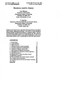
Where C = —[sin(ka)cos{qbo) + cos(ka)sin{qbo)]/\2sin{K)\, and \C\ is larger than but very close to 1 when wavelength is at the band center, and become bigger when wavelength ap­ proached the band edge. So the slope of In T vs L for a short periodic system is almost same as the negative value of the slope for the long system. The slopes of In T at both sides of the maximum are approx­ imately symmetric. In Fig. la, we can see that, when L < L°, T increases vs L with the slope l / f £ , and get t o a maximum a t L° C and decays exponentially when L > L° with the slope 1/ÇIFrom the behavior of the theoretical expressions of T or R , when T or R goes to infinite, we can obtain analytically that L° is given as:

(10)

where C is same as defined above in Eq.(9), and |C| is close to one. From the property of \C\ discussed above, we can see that lPc »

at the band center , and becomes smaller when

wavelength approaches the band edge. The value of \C\ is almost independent of gain, so

is

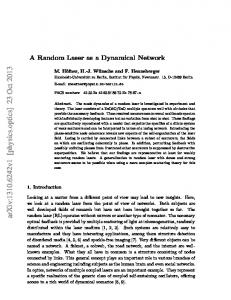
parallel to 1/s" or ^. We have shown that Lqce" is almost a constant for a given wavelength, and our numerical results agree very well with the theoretical prediction. The reflection coefficient gets to a maximum value at

too, and fluctuates a lot with the

size L of the system. When L approaches infinity, R reaches a saturated value. The saturated value of R is given by:

&«—-iSiSrS So RQ is almost independent of gain or £i. Fig. 2 shows that indeed R increase when L < gets to its maximum value and fluctuate violently at which is almost independent of gain.

then approaches a saturated value

32

Electronic tight-binding model For the electronic tight-binding model, when E = 0, the In T for the long system can be obtained by the use of Eq.(7):

Sl NÎF = -L/îi - -I



Similarly as the classical many-layered model, for short system of tight-binding model we have:

=

-77

(13)

So the slope symmetry of In T at both sides of LQC still exists. In Fig. lb, we can see a similar behavior as in Fig. la, when L
L C . When L/Ç L > l / £ 0 and L < L C ,

33

< InT > increase vs L from origin with a slope which is defined as !/£' and when L > L C , < In T > decrease vs L with a slope —l/£. But when 1/fi < l/£o, < InT > will decrease monotonically, at first with the slope 1/Çi = — l/|fi|, at LC, there are a turning point and slope changes to —1/Ç. We will study the values of Ç' , Ç and LC in this section. It was first suggested by Zhang [8] that the localization length £ of a long random system with gain will become smaller than the localization length £o of the random system without gain. In particular he suggested that:

(15)

where £o is the localization length of the system without gain, lg is replaced by

in the original

formula of Zhang because of the periodic background of our systems. We have numerically calculated l/£ for different cases of disorder, gain and frequency (energy), and compare it with l/£o + 1/fi, as shown in Fig. 5a and 5b for the many-layers model and the tight-binding model respectively. For most of the cases, Eq.(15) is a very good formula. Only when wavelength is on band edge and when both gain and randomness are very strong, we can see that the numerical results deviate from the theoretical prediction, which is the solid line in both Fig. 5a and 5b. For short system(L < Lc), the behavior of < In T > vs L is quite different from that of long system as shown in Fig. 4. Freilikher et.al. and Rammal and Doucot [17] obtained that the transmission coefficient of a random system with absorption is given by:

< InT >= {-y- — t~)L 'a SO

(16)

where la is the absorption length and £o is the localization length. For a medium with gain, can we just substitute the —la~l with lg~l in the Eq.(16) to get following equation?

(17)

34

Because of the periodic background of our models, we use £1 to replace lg in our calculations. So far there is no independent verification for this conclusion. After substituting £1 for lg, our numerical results show that Eq.(17) is correct for short systems with gain for both models. When the strength of the disorder is a constant , so Çq is a constant, according to Eq.(17), l/£i — 1/Ç' should be equal to l/£0 and be constant as the gain varies. We have checked this prediction and find indeed that the numerical values are almost the same as the ones predicted theoretically. From Eq.(17), we can predict the basic features of the length dependence of < lnT > shown in Fig. 4. When 1/Çi > I/Co, < In T > will increase with L, and will reach a maximum value when L gets to LC. But if 1/fx < I/Ç01 the < In T > will decrease monotonically, at first with a slope of — |l/£i — l/fo| from the origin, at LC the curve has a turning point and the slope changes to — |l/£i + l/£o|- If 1/Çi ~ l/£o, the curve is almost horizontal for small L and begins to decrease with a slope —1/Ç at the critical length. This behavior is exactly shown in Fig. 4. The critical length L C is one of the most important parameters of a random system with gain. For a random system, one of the most important theories is the Letokhov theory [6], Zhang [8] generalized the theory and used the no-gain localization length £o to replace the diffusion coefficient D in the Letokhov theory and obtain that the critical length LC ~ \/ from the value of !/£', such as: if it is positive then the < In T > will increase from origin at slope !/£' and generate a peak at Lc and then start to decrease at slope —1/Ç, if it is negative then the < In T > will decrease monotonically and has a turning point at Lc with the slope change from

to — 1/Ç.

To explain the new behavior of the critical length L c which we got from our numerical results, we compare the Letokhov theory with the Lamb theory and give a general expression for the critical length considering both the effects of localization and periodic background. With this comparison, we also construct the relation of the quality factor Q of a random system with the localization length Ç. We also study the probability distribution of the reflection coefficient P ( R ) of random systems with gain. We find some new behaviors of P{R) and give the criteria for the range of validity of the different behaviors and explain it by the influence of the periodic background too. The study of wave propagation in amplifying random system is a new and challenging topic. There are still a lot things to be done.

Acknowledgment Ames Laboratory is operated for the US Department of Energy by Iowa State University by Iowa State University under Contract No.W-7405-Eng-8'2. This work was supported by the Director for Energy Research office of Basic Energy Sciences and Advanced Energy Projects and by NATO Grant No.940647. Bibliography [1] P. W. Anderson, Philos. Mag. B 52, 505 (1985) [2] S. John, Phys. Rev. Lett. 53, 2169 (1989); also S. John, Phys. Today 44(5) , 32 (1991) [3] C. M. Soukoulis, E. N. Economou, G. S. Grest, M. H. Cohen, Phys. Rev. Lett. 62, 575 (1989); E. N. Economou and C. M. Soukoulis, Phys. Rev. B 40, 7977 (1989)

41

[4] J. Kroha, C. M. Soukoulis, and P. Wolfle, Phys. Rev. B 47, 11093 (1993) [5] N. M. Lawandy et.al. , Nature 368, 436(1994); D. S. Wiersma, M. P. van Albada and Ad Lagendijk, Phys. Rev. Lett. 75, 1739 (1995) [6] V. S. Letokhov. Sov. Phys. JETP 26. 835 (1968) [7] C. W. J. Beenakker, J. C. J. Passchens, and P. W. Brouwer, Phys. Rev. Lett. 76, 1368 (1996); P. Pradhan, N. Kumar, Phys. Rev. B. 50, 9644 (1994) [8] Z. Q. Zhang, Phys. Rev. B. 52, 7960 (1995) [9] J. C. J. Paasschens, T. Sh. Misirpashaev and C. W. J. Beenakker, Phys. Rev. B 54, 11887 (1996) [10] A. Yu. Zyuzin, Europhys. Lett. 26, 517 (1994) [11] A. Yu. Zyuzin, Phys. Rev. E. 51, 5274 (1995) [12] A. K. Sen, Modern Phys. Lett. B. 10 125 (1996) [13] S. K. Joshi, A. M. Jayannavar, Phys. Rev. B. 56, 12038 (1997) [14] G. Bergmann, Phys. Rev. B. 28, 2914 (1983) [15] Amnon Yariv, Optical Electronics in Modern Communications (Oxford Univ. Press, New York,1997) [16] M. Sargent III, M. O. Scully, and W. E. Lamb. Jr, Laser Physics (Addison-Wesley, Read­ ing, Mass., 1974). or, K.Shimoda, Introduction to Laser Physics (Springer-Verlag, Berlin Heidelgerg New York, Tokyo, 1984) [17] R. Rammal, B. Doucot, J. Phys. (France) 48, 509 (1987); V.Freilikher, M. Pustilnik, and I. Yurkevich, Phys. Rev. Lett. 73, 810 (1994) [18] Xunya Jiang, Qiming Li, C. M. Soukoulis, unpublished

42

20

10

Do

o

0

% -10 -10

(L-^,

Figure 1 The logarithm of the transmission coefficient t versus ( l — l ° ) / ç i , where L° is the critical length and is the gain length of peri­ odic systems, (a) For the periodic many-layered model, (i), (ii) and (iii) are the values at three representable wavelength A= 360 nm(band center), 420 nm (general) and 470 nm(band edge) re­ spectively. The different symbols represent values obtained from different gains, s" = -0.001, -0.002, -0.005, -0.001, -0.1. (b) For the periodic tight-binding model with E=0 for different gains 77=0.01, 0.05, 0.1, 0.2, 0.5.

43

20

2130

1060

21 214 426 10 0 10 •20

1000

0

2000

3000

2000

3000

1000

1500

20 122

10

265

1248

644

0 10

20 0

1000

20 412

10 0 10 •20

0

Figure 2

500

The logarithm of the reflection coefficient r versus L for the pe­ riodic many-layered model, (a), (b) and (c) are values of three representative wavelengths x— 360 nm, 420 nm and 470 nm re­ spectively. From right to left, the numbers on the peaks are the values of corresponding to different gains e" = -0.001, -0.002, -0.005, -0.01, -0.1. Notice that the saturated value of R is inde­ pendent of e" for the three wavelengths studied.

44

i S1731 1 III IL

^ Mm*"

1W^AY1""

r'

1

(a)

0

100

1 200

1

300

145 s/ is al­ most horizontal for small L, as shown by the wide solid line. For e" > 0.001, l/£i > 1/fo, and for e" < 0.001, 1/fi < 1/fo- Results for the random tight-binding model, with E = 0 and W = 1, are shown by dashed lines. Lines from lower to higher correspond to T}= 0.01, 0.02, 0.08, 0.3. When 77 is equal to 0.02, 1/Çi is almost same as 1/Ço, so < In T > is almost horizontal for small L, as shown by the wide dashed line. For 77 > 0.02, 1/Çi > 1/Ço, and for 77 < 0.02, 1/fi < 1/fo-

10

46

3JLP

Figure 5

1/Ç.+14 l/£ versus to 1/Ço + 1/fi, where Ç is localization length for a system with gain, £0 is the localization length of a system with disorder but with zero gain, and £1 is the gain length, (a) For the random many-layered model, empty symbols are of wave­ length A=360 nm, filled symbols are of A=470 nm. Different symbols represent different sets of parameters of disorder and gain, W = 0.05,0.1,0.2,0.5; £"=0.001, 0.002, 0.005, 0.01, 0.05, 0.1. (b) For the random tight-binding model, empty symbols are of energy E = 0, filled symbols are of energy E = 1.8. Differ­ ent symbols represent different sets of parameters of disorder and gain, W=0.5, 0.8, 1, 1.5, 2, 3, 5; t?=0.01, 0.05, 0.1, 0.3.

47

1000

800 O Numerical Results

600

L=(S,S/q.7)'*

1/2

- L=-C+(Ç2+(^/0.7))

400

200

B-

0.0 200

0.4

0.2

150

0.6

0.8

1.0

o Numerical Results L,=%/0.7r - L=-^ 2 HUJ0.7)f 2

100

50

0

1

2

3

w Figure 6 The critical length l c is plotted versus different random strengths W. (a) For the random many-layered model with A=360nm, the dashed line and darkened line are the values obtained according to Zhang's formula and Eq.(25) respectively, (b) For the ran­ dom tight-binding model with e=0 and 77=0.01, the dashed line and darkened line are the values obtained according to Zhang's formula and Eq.(25) respectively. In both cases C = 2^i'° aiK* a = 0.7.

4

48

d

1000 Figure 7

2000

3000

4000

Probability distribution of the reflection coefficient P(x) versus x of the random many-layered system with gain at A = 300 nm for q — 1.1 and 17.7 (a); q = 0.163 (b); q = 451 (c), where x = (R — 1 )/q and q = £o/£i- The solid curve given by the solid line in (a), (b) and (c) is the analytical result of Eq.(26). In (d), P(R) versus R is plotted for two values of q , q = 1800(low one) and 7200(high one). Notice that P(R) ap­ proaches a delta-function distribution at RQ when q = 7200.

5000

49

0.8

0.8

0.6

0.6

0.4

0.4

0.2

0.2

0.0

2

1

0

0.0 3

4

2

1

0

3

4

0.20 0.8

0.15

0.6 0.10 0.4 0.05

0.2 u

0.0 0

!

1 Figure 8

,

^

1

2

3

.

0.00

4

1500

'

1

1550

Li

1600

Probability distribution of the reflection coefficient P(x) versus x of the random tight-binding system with gain at E = 0 for q = 1.0 (a); q = 132 (b); q = 525 (c), where x = (R — 1)/q and q = £o/fiThe solid curve given by the solid line in (a), (b) and (c) is the analytical result of Eq.(26). In (d), P(R) versus R is plotted for q = 5.25 x 104- P{R) approaches a delta-function distribution at Ro when q = 5.25 x 104.

1650

50

CHAPTER 3. IS THERE A SYMMETRY BETWEEN ABSORPTION AND AMPLIFICATION IN DISORDERED MEDIA?

A paper published in the journal of Physical Review B rapid communitcation Xunya Jiang, Qiming Li, and Costas M. Soukoulis

Abstract Previous studies found a surprising symmetry between absorption and amplification in dis­ ordered one-dimensional systems once the system size exceeds certain thresholds. We show that this paradoxical result is an artifact due to the assumption of a finite output in solving the time-independent wave equation, when in fact both the transmission and the reflection amplitude are divergent as a result of the large amplification. More sophisticated approaches, such as time-dependent equations including field and matter coupling have to be utilized to correctly describe the wave propagation of systems with large sizes.

Intro duction Recent observations [1] of laser-like emission from dye solution immersed with TiC>2 nanoparticles have stimulated intensive theoretical efforts [2, 3, 4, 5, 6, 7, 8, 9, 10, 11, 12, 13] to investigate the properties of disordered media which are optically active. With enhanced op­ tical paths from multiple scattering, random systems are expected to possess a reduced gain threshold for lasing[14, 15]. Correspondingly, one would expect the transmission in disordered

51

systems to be enhanced with gain. Surprisingly, transfer matrix calculations^, 4] based on time-independent wave equations showed that for large systems the wave propagation is ac­ tually suppressed with gain, leading to enhanced localization[16, 17] of waves as if the system is absorbing. Subsequently a more rigorous proof[5] for such a symmetry between absorption and amplification was presented for the time-independent wave equation. Intuitively one would expect that the presence of amplification should facilitate wave prop­ agation, not suppress it, even in disordered systems. At least in the weak scattering (diffusive) regime, amplification always enhances wave transmission^, 14, 15, 18]. The time-dependent diffusion equation predicts an increased output and a gain threshold above which the system become unstable[14, 15, 18]. The diffusive description of photon transport in gain media ne­ glects the phase coherence of the wave. Thus it was generally believed that the paradoxical phenomenon may indicate enhanced localization due to interference of coherently amplified multiply reflected waves[3, 4, 5, 6, 8, 10, 11, 13]. However, amplification of backscattering does not necessarily imply a reduction in transmission because no conservation of the total photon flux is required in gain media. With sufficient gain, wave should be able to overcome losses from backscattering and propagate through the system with increased intensity. To fully un­ derstand the origin of this apparent non-intuitive suppression of transmission, we will examine the validity of the solutions derived from the time-independent wave equation which has been commonly employed in describing the wave propagation in active media. Linearized time-independent wave equations with a complex dielectric constant have been successfully utilized to find lasing modes by locating the poles[19] in the complex frequency plane and to investigate the spontaneous emission noise below the lasing threshold in dis­ tributed feedback semiconductor lasers[20, 21]. Such equations are known to be inadequate[19, 20] to describe the actual lasing phenomena due to their simplicity in dealing with the interac­ tions between radiation and matter. However, it is generally believed that the time-independent equation should suffice to describe the wave propagation in amplifying media, before any os­ cillations occur. We will unambiguously show that the so-called symmetry [4, 5] between amplification and absorption is an artifact due to the unphysical assumption of a finite output

52

in solving the time-independent wave equations, when such solutions cease to exist at large lengths or large gain. We will show that for each system, there is a frequency-dependent gain threshold above which no stable time-independent output exists. Solving the time-independent wave equations by incorrectly assuming a fixed output leads to unphysical solutions that does not correspond to the true behavior of the system. These conclusions are supported by nu­ merical solutions of the time-dependent wave equation with a semi-infinite planewave incident upon a linearly amplifying media.

Theoretical Model and Derivation To see how the unphysical solution could arise from the time-independent equation, we take the simplest example of wave propagation through a uniform active media-the classical Febry-Perot setup with the two interfaces acting as feedback mirrors (see the insert in Fig. 1). The time-independent wave solution must satisfy the wave equation,

^

+

£

w s w =

where E(z) is the electric field and the dielectric constant

o.

E(Z)

m = e'(z) — ie"(z) is complex with

the imaginary part signifying amplification from stimulated emission of radiation (e" > 0) or absorption (s" < 0 ). Here we have assumed a constant e" independent of field intensity to represent a uniform linearly amplifying media. We also comment that in electromagnetic theory, the imaginary part of the dielectric constant is proportional to the conductivity of the material and thus cannot be negative. The negative dielectric constant is strictly speaking only an phenomenological way to introduce coherent amplification [22]. Complex potentials known as optical potential have long been employed in nuclear physics to describe inelastic nuclei scattering processes[23]. For time-independent solutions, the field inside and outside the media are plane waves, with amplitude given as in the inset of Fig. 1. The transmission and the reflection amplitude can be easily obtained by matching the boundary conditions at the two interfaces, with the

53

final expression,

(2) where t\ = 2k/(k + &o), t 2 = 2ko/(k + ko), and ry = r 2 = (k — ko)/(k + ko) are the effective transmission and reflection coefficients at the left and right two interfaces(mirrors), respectively. ko = y/eô^ and k = k' — ik" = \/e' — is"^ are the wavevectors outside and inside the system, respectively. L is the distance between the "mirrors". The oscillation condition for lasing is correctly given by 1 — rir2e2tkL = 0 at which both the transmission and reflection coefficient diverge.

However, Eq.(2) also predicts the ex­

ponential decrease of the transmission amplitude for large system sizes, asymptotically as (t| ~ \exp{—ikL)\ = exp{—k"L). This is clearly shown in Fig.l, where we plot ln(T) versus L. Notice that for large L, ln(T) decreases as L increases despite the fact that the system has gain. Gain effectively becomes loss at large lengths! Remember the system is homogeneous thus disorder is definitely not responsible for this strange behavior. We see that the inhibition of wave transmission for large systems is clearly not unique to disordered systems [7] and could not possibly come from the amplification of backscattering. A more illuminating picture of what is going on can be obtained from the path integral method [19]. In such an approach, the total transmission coefficient can be obtained by adding coherently contributions from all paths of successively reflected and transmitted rays. We obtain a sum of geometrical series, t = ht 2 e i k L {1+ (r i r 2 e 2 i h L ) + { r i r 2 e 2 i k L ) 2 + •••].

(3)

The first term represents the direct transmission of the incoming wave, and the second term represents the wave which was reflected first by r2 at the right interface and then by ri at the left interface and subsequently transmitted through (see inset of Fig. 1). More terms from sequences of multiple transmissions and reflections at the left and right "mirrors" follow. Eq. (3) can be interpreted physically as the output at long times when an continuous planewave are incident upon the system. It is a simple matter to verify that Eq.(3) indeed reproduces Eq. (2), provided that the

54

following condition is met, \r x r 2 e 2 l k ' L e 2 k " L \ < 1.

(4)

When the condition given by Eq. (4) is violated, such as when the system size or the gain is large, the output represented by the sum fail to converge, indicating physically the absence of a stable time-independent solution. The divergence of the transmission above threshold even away from the oscillation pole is the key in understanding the failure of Eq.(2), which is conventionally derived from boundary condition matching by implicitly assuming that the output is always finite.

Normally the

physical boundary condition is satisfied when t\t2elkL + r1r2e2,fc££ = £, resulting in Eq. (2). Obviously this condition cease to be meaningful when t is not finite or ill-defined. Consequently, Eq. (2) cease to represent the physical output. In contrast the condition given by Eq.(4) is always satisfied for lossy media. The non-convergence of output is a unique phenomenon occurring only to systems with gain. The breakdown of the time-independent wave equation at large gain or large system sizes signals the large fluctuations of the transmission in time and calls for more sophisticated theories that can take into account in more detail the interaction between radiation and matter to correctly describe the response of the system. Numerical Results of FDTD Model To support our picture, we have studied the transmission problem of the simple Febry-Perot system directly by solving numerically the time-dependent equation with a well-developed finite-difference-time-domain

(FDTD) technique [24]. A semi-infinite planewave of a fixed

frequency is incident upon the system from the left. Absorbing boundary conditions have been applied on both end to eliminate the reflection at the boundaries. We choose A = 800 nm and L=4300nm.The dielectric constant outside is taken to be £o = 1 and the real part of the dielectric constant of the active media is £ = 9. Both mirrors have been chosen to be reflectionless for simplicity (the interfaces provide feedback). For this system, the threshold gain is calculated to be e" = 0.12 from Eq. (4). In Figure 2, we show the field amplitude immediately outside of the active medium as a function of time, for different values of amplification (and

55

absorption). The time unit to here is the round trip time of the light within the media. We expect after some transient time, the transmitted wave should converge to the solution Eq. (2) predicted by the time-independent equation. This is indeed what happens when the gain is below the threshold. However, when the gain is above the threshold, the output field appears to increase with time exponentially without bound, indicating the non-existence of a stable time-independent solution under these conditions. We have also performed similar calculations on a random system consisting of 50 cells of binary layers with £q = Si = 1 and £2 = 4 — is

Within the unit cell the thickness of the

first layer is a random variable an = ao(l + Wy) where oq = 95nm. W = 0.8 and

7

is a

random value in the range [-0.5, 0.5]. The cell length is fixed to be 215nm. The wavelength of the incident wave is À = 1200nm. The results are shown in Fig. 3. Again we see the output field strength increases with time without any bound once the gain reaches some value. This threshold depends not only on frequency but also on disorder configuration of the sample. Fig. 3 clearly show the output always increases with gain for the same input and there is no sign of the suppression of transmission, even in random systems. These numerical solutions demonstrate unambiguously that for a linearly amplifying medium, there is a frequency-dependent and sample-specific gain threshold above which no physical time-independent solution exists. Solutions from the time-independent equation are valid only below the threshold. This threshold decreases with increasing system size. Unfortunately it is difficult to determine this threshold without explicitly solving the time-dependent equation. One certainly cannot tell from the expression of the total transmission coefficient itself since it is well behaved except exactly at the discrete oscillation poles. One method is to divide the whole system into smaller subsystems and then apply the geometrical sum of multiple reflections and transmission technique, as we have done for the Febry-Perot set up, to each subsystem to find the threshold curve for the subsystem. Then the locus formed by all the possible subsystem will be the threshold curve for the whole system. However, this strategy is practical only to simple systems. It is very difficult to carry out such analysis for large or disordered systems. However, since the oscillation poles for the lasing threshold are still

56

correctly given by the divergence of the transmission coefficients from the time-independence solutions, an estimate of the magnitude of the threshold for frequencies away from the pole can be obtained from the threshold values of nearby lasing poles. A study of the distribution of these poles has been carried out for a random layer system by carefully locating the pole posi­ tion by continuously tuning the gain up at a fixed frequency until the transmission coefficient from the time-independent equation diverges[9]. The implication of our analysis is that the calculation of transmission and reflection coef­ ficient with the traditional method from time-independent equations become suspect once the gain or system size reaches a certain value. Care has to be taken to ensure that the system is not above the threshold and the solution physical. This remark not only applies to studies with transfer matrix[4, 5, 6, 7, 8, 10, 12, 13] but also pertains to the application of the powerful invariant embedding method[25] which has been widely employed in the studies[3, 6, 8, 11] of transmission problem in random gain media. The presence of a stable time-independent solution is implicitly assumed in these approaches. Consequently, the conclusions of previous studies[3, 4, 6, 8, 10, 11, 13] on the statistical properties of the transmission and reflection coefficient need to be re-evaluated in light of the current finding. Conclusion In summary, we show that amplification does not suppress wave transmission, as has been claimed previously for random active media. On the contrary, it always enhanced wave prop­ agation. Numerical solution to the time-dependent equation show when the system size (or gain) reaches a frequency and configuration dependent threshold, both the amplitude of the reflected and the transmitted wave from a continuous input increases with time without any bound. The erroneous conclusions reached in precious studies was an artifact of the failure of the output wave to converge to a finite value, which must be assumed in any solutions of the time-independent equation. In light of the current findings, some of the conclusions on the statistical properties of the reflection and the transmission coefficient in media with gain become suspect, especially at large system sizes. The time-independent equation is inadequate

57

to describe the amplification of light under these conditions. Nevertheless, the simplicity of the time-independent equation can still be used effectively to locate resonant conditions, even in disordered systems. A complete treatment of the wave propagation in gain media may require the construction of the time-dependent solution out of the continuous and discrete solutions of the time-independent equation[26]. Unlike for the Hermitian system, the completeness of these solutions could not be proved easily when the potential is complex. Ames Laboratory is operated for the U.S. Department of Energy by Iowa State University under Contract No. W-7405-Eng-82. This work was supported by the director for Energy Research, Office of Basic Energy Sciences. Bibliography [1] N. M. Lawandy, R. M. Balachandran, S. S. Comers, and E. Sauvain, Nature 368, 436 (1994); D. S. Wiersma, M. P. van Albada and Ad Lagendijk, Phys. Rev. Lett. 75, 1739 (1995). [2] S. John and G. Pang, Phys. Rev. A 54, 3642 (1996), and references therein. [3] P. Pradhan, N. Kumar, Phys. Rev. B 50, 9644 (1994). [4] Z. Q. Zhang, Phys. Rev. B 52, 7960 (1995). [5] J. C. J. Paasschens, T. Sh. Misirpashaev and C. W. J. Beenakker, Phys. Rev. B 54, 11887 (1996). [6] A. K. Gupta and A. M. Jayannavar, Phys. Rev. B 52, 4156 (1995). [7] A. K. Sen, Mod. Phys. Lett. B 10, 125 (1996). [8] C. W. J. Beenakker, J. C. Paasschens, P. W. Brouwer, Phys. Rev. Lett. 76, 1368 (1996). [9] Qiming Li, K. M. Ho, and C. M. Soukoulis, unpublished. [10] S. K. Joshi and A. M. Jayannavar, Phys. Rev. B 56, 12038 (1997).

58

[11] K. Kim, Phys. Rev. B 58, 6153 (1998). [12] X. Y. Jiang, C. M. Soukoulis, To appear in Phys. Rev. B. [13] P. Pradhan, Cond-mat/9807312. [14] V. S. Letokhov, Sov. Phys. JEPT 26, 835 (1968). [15] A. Yu. Zyuzin, Europhys. Lett. 26, 517 (1994). [16] P. W. Anderson, Philos. Mag. B 52, 505 (1985). [17] S. John, Phys. Today 44(5), 32 (1991). [18] A. A. Burkov and A. Yu. Zyuzin, Cond-mat/980422. [19] A. Yariv Optical Electronics in Modem Communications (Oxford Univ. Press, New York, 1997). [20] C. H. Henry, J. Lightwave Technology, LT-4, 288 (1986). [21] T. Makino and J. Glinski, IEEE J. Quantum Electron. 24, 1507 (1988). [22] M. Sargent III, M. O. Scully, and W. E. Lamb. Jr, Laser Physics (Addison-Wesley, Read­ ing, Mass., 1974). [23] L. D. Landau, E. M. Lifshitz Quantum Mechanics (Third edition 1987). [24] A. Taflove, Computational Electrodynamics (Artech House, London, 1995). [25] R. Rammal and B. Doucot, J. Phys. (France) 48, 509 (1987). [26] E. N. Economou, private communication.

59

50000

100000

Figure 1 The logarithm of the transmission coefficient, ln(T), versus the length L of a simple Febry-Perot setup. The dielectric constant of the Febry-Perot device is s — s' — is" = 2 — z'0.01. The dielectric constant of the outside medium is s = 1 without gain. In the insert a schematic representation for the wave transmission in a simple Febry-Perot setup is shown.

150000nm

60

0 £"=0.24 a £ =0.217 e £"=0.18

V

à £"=0.15 V E =0.1 £"=0.

• £"=-0.24

tit. Figure 2

The logarithm of output at the right side of system versus time of a Febry-Perot setup with a planewave(A = 800 nm) incidence. The length of system is the l = 4300 nm and the dielectric con­ stants of the inside and outside materials are £i = 9 — ie" and £\ — 1, respectively. The time unit to is the round trip time for the wave to travel through the medium. The critical gain of the system on this frequency is e" = 0.12.

61

Q €'=0.0216

* £"=0.0144 o €'=0.00720 & £"=0.00360 £"=0

* £ =-0.0144

400

Figure 3

The logarithm of output at the right side of system versus time of a random system with a planewave(A = 1200 nm) incidence. The system consists of 50 cell of binary dielectric media with £i = 1 and £2=4 — ie" respectively. The cell length is fixed at 215 nm and the length of the first medium is given by a n = OQ (1 + W~f), where cq = 95 nm, W = 0.8 and 7 is a random number between (—0.5,0.5). The time unit to is the round trip time for the wave to travel through the system. The critical gain of this system on this frequency is about e" = 0.0031.

62

CHAPTER 4. TIME DEPENDENT THEORY FOR RANDOM LASERS

A paper published in the journal of Physical Review Letter Xunya Jiang and C. M. Soukoulis

Abstract A model to simulate the phenomenon of random lasing is presented. It couples Maxwell's equations with the rate equations of electronic population in a disordered system. Finite dif­ ference time domain methods are used to obtain the field pattern and the spectra of localized lasing modes inside the system. A critical pumping rate P£ exists for the appearance of the lasing peaks. The number of lasing modes increase with the pumping rate and the length of the system. There is a lasing mode repulsion. This property leads to a saturation of the number of modes for a given size system and a relation between the localization length £ and average mode length l m .

Introduction The interplay of localization and amplification is an old and interesting topic in physics research [1]. With promising properties, mirror-less random laser systems are widely studied [2, 3, 4, 5, 6, 7] both experimentally and theoretically. Recently new observations [2] of laser-like emission were reported and showed new interesting properties of amplifying media with strong randomness. First, sharp lasing peaks appear when the gain or the length of the system is over a well defined threshold value. Although a drastic spectral narrowing has been previously

63

observed [3], discrete lasing m-odes were missing. Second, more peaks appear when the gain or the system size further increases over the threshold. Third, the spectra of the lasing system is direction dependent, not isotropic. To fully explain such an unusual behavior of stimulated emission in random systems with gain, we are in need of new theoretical ideas. Based on the time-dependent diffusion equation, earlier work of Letokhov [l] predicted the possibility of lasing in a random system and Zyuzin [5] discussed the fluctuation properties near the lasing threshold. Recently, John and Pang [6] studied the random lasing system by combining the electron numboer equations of energy levels with the diffusion equation. By using the diffusion approach iss not possible to explain the lasing peaks observed in the recent experiments [2] in both semiconductor powders and in organic dyes-doped gel films. Another approach which is based on tlie time-independent wave equations for the random gain media can go beyond the diffusive description [7, 8, 9, 10, 11], but is only useful in determining the lasing threshold [12]. To fulhy understand the random lasing system, we have to deal with time-dependent wave equatioms in random systems by coupling Maxwell's equations with the rate equations of electron pop*ulation within a semi-classical [13, 14] theory. In this paper we introduce a model by combining these semi-classical laser theories with Maxwell's equations. By incor porating a well-established FDTD ( finite-difference time-domain) [15] method we calculate the vwave propagation in random media with gain. Because this model couples electronic number equations at different levels with field equations, the amplification is nonlinear and saturated, so stable state solutions can be obtained after a long relaxation time. The advantages of this FDTD model are obvious, since one can follow the evolution of the electric field and electron mumbers inside the system. From the field distribution inside the system, one can clearly distinguish the localized modes from the extended ones. One can also examine the time dependence of the electric field inside and just outside the system. Then after Fourier transformation, the emission spectra and the modes inside the system can be obtained.

64

FDTD model Our system is essentially a one-dimensional simplification of the real experiments [2, 3]. It consists of many dielectric layers of real dielectric constant of fixed thickness, sandwiched between two surfaces, with the spacing between the dielectric layers filled with gain media (such as the solution of dye molecules). The distance between the neighboring dielectric layers is assumed to be a random variable. The overall length of the system is L. Our results can be summarized as follows: (i) As expected for periodic and short (L < £, Ç is the localization length) random system, an extended mode dominates the field and the spectra. (ii) For either strong disorder or the long (L

0 system, we obtain a low threshold

value for lasing. By increasing the length or the gain more peaks appear in the spectra. By examining the field distribution inside the system, one can clearly see that these lasing peaks are coming from localized modes. (Hi) When the gain or the pumping intensity increases even further, the number of lasing modes do not increase further, but saturate to a constant value, which is proportional to the length of system for a given randomness. And (iv) the emission spectra are not same for different output directions which show that the emission is not isotropic. These findings are in agreement with recent experiments [2] and also make new predictions. We want to point out that our model is ID unlike the experiments which are done in 3D samples. However, the experimental results are strongly dependent on the shape of the excitation area [2], Sharp lasing peaks are observed only if the excitation area is stripe like, which is close to our ID model. In the ID case we expect the number of lasing modes to be less than the 3D case but much sharper. This is due to the fact that the modes are more localized and there are less propagating paths in ID. The binary layers of the system are made of dielectric materials with dielectric constant of

Si

=

SQ

and e2 = 4 x £Q respectively. The thickness of the first layer, which simulates the

gain medium, is a random variable an = oq(1 + W-y) where oq = 300nm, W is the strength of randomness and 7 is a random value in the range [-0.5, 0.5]. The thickness of second layer, which simulates the scatterers, is a constant b = 180nm. In the layers representing the gain medium, there is a four-level electronic material mixed inside. An external mechanism pumps

65

electrons from ground level (iV0) to third level (AT3) at certain pumping rate Pr, which is proportional to the pumping intensity in experiments. After a short lifetime 732, electrons can non-radiative transfer to the second level (iV2). The second level (iV2) and the first level (iV*i) are called the upper and the lower lasing levels. Electrons can be transfered from the upper to the lower level by both spontaneous and stimulated emission. At last, electrons can non-radiative transfer from the first level (Ni) back to the ground level (Wo). The lifetimes and energies of upper and lower lasing levels are r21, £2 and r10, Ei respectively. The center frequency of radiation is u a = (E 2 — E\)/h which is chosen to be equal to 2 tt x 6 • 10 1 4 Hz . Based on real laser dyes [16], the parameters t32, r21 and r10 are chosen to be 1 x 10~13s, 1 x 10~9s and 1 x 10-11s. The total electron density N° = No + Ni + N2 + N3 and the pump rate Pr are the controlled variables according to the experiments [2]. The time-dependent Maxwell equations are given by V x E = — d~B/dt and V x H = edE/dt + dP/St, where B =

/J.H

and P is the electric polarization density from which the

amplification or gain can be obtained. Following the single electron case, one can show [14] that the polarization density P(x, t) in the presence of an electric field obeys the following equation of motion:

^S^+Aa,a^Sr+u,-p(i) =

(1)

where Au>a = l/r2i+2/T2 is the full width at half maximum linewidth of the atomic transition. T 2 is the mean time between dephasing events which is taken to be 2.18 x 10 - 1 4 s, AN(x,t) = Ni(x,t) — N2(x,t) and jr = l/r21 is the real decay rate of the second level and yc = ^6^c3 is the classical rate. It is easy to derive [14] from Eq. (1) that the amplification line shape is Lorentzian and homogeneously broadened. Eq. (1) can be thought as a quantum mechanically correct equation for the induced polarization density P(x,t) in a real atomic system. The equations giving the number of electrons on every level can be expressed as follows:

dN 3 (x, t) #3(2, () = P r No(x,t) — dt T32

66

dN 2 (x,t) dt

_

N 3 (x,t) | E(x,t) dP(x,t) 7*32 hu>a dt

N 2 (x,t) T2i (2)

dNi(x, f) dt

_

where

d P

E(x,t) dP(x,t) Awg A A^l_ PrAfo(l . t) Tio T2 i

=

at

#2(2, t)

Ni(x,t) rI0

£ i s the induced radiation rate or excitation rate depending on its sign.

To excite the system, we must introduce sources into the system [IT]. To simulate the real laser system, we introduce sources homogeneously distributed in the system to simulate the spontaneous emission. We make sure that the distance between the two sources Ls is smaller than the localization length £. Each source generates waves of a Lorentzian frequency distribution centered around uia, with its amplitude depending on N2.

In real lasers, the

spontaneous emission is the most fundamental noise [13, 14] but generally submerged in other technical noises which are much larger. In our system, the simulated spontaneous emission is the only noise present, and is treated self-consistently. This is the reason for the small background in the emission spectra shown below. There are two leads, both with width of 300 nm, at the right and tlie left sides of the system and at the end of the leads we use the Liao method [15] to impose absorbing-boundary conditions (ABC). In the FDTD calculation, we discretize both the space and time, the discrete time step and space steps are chosen to be 10-17s and 10~9m respectively. In the FDTD scheme the boundary conditions for the field at the interfaces between the two media are automatically satisfied, since we are numerically solving Maxwell's equations. So far a given random configuration, based on the previous time steps we can calculate the next time step (n + 1 step) values. First we obtain the n + 1 time step of the electric polarization density P by using Eq. (1), then the n + 1 step of the electric and magnetic fields are obtained by Maxwell's equations and at last the n + 1 step of the electron numbers at each level are calculated by Eq. (2). The initial state is that all electrons are on the ground state, so there is no field, no polarization and no spontaneous emission. Then the electrons are pumped and the system begins to evolve according to the above equations.

67

Numerical Results and Theoretical Discussion We have performed numerical simulations for periodic and random systems. First, for all the systems, a well defined lasing threshold exists. As expected, when the randomness becomes stronger, the threshold intensity decreases because localization effects make the paths of waves propagating inside the gain medium much longer. For a periodic or short (L < £) random system, generally only one mode dominates the whole system even if the gain increases far above the threshold. This is due to the fact that the first mode can extend in the whole system, and its strong electric field can force almost all the electrons of the upper level

to jump down to the Ni level quickly by stimulated

emission. This leaves very few upper electrons for stimulated emission of the other modes. In other words, all the other modes are suppressed by the first lasing mode even though their threshold values are only a little bit smaller than the first one. This phenomenon also exists in common homogeneously broadening lasers [13]. For long {L » £) random systems, richer behavior is observed. First we find that all the lasing modes are localized and stable around their localization centers after a long time. Each mode has its own specific frequency and corresponds to a peak in the spectrum inside the system. When the gain increases beyond the threshold, the electric field pattern (see Fig. la) shows that more localized lasing modes appear in the system and the spectrum intensity Ie inside the system (see Fig. Id) gives more sharp peaks just as observed in the experiments [2]. Notice that N2 is small (Fig. 2b) in the position where the amplitude of the electric field Ae (Fig. la) is large, and this is because of the stimulated emission. In Fig. lc, the time dependence of the averaged Ae over all the spatial points is shown. Ie is obtained by taking the Fourier transform of the spatial averaged A#(t). The exact position of the lasing peaks depends on the random configuration. Notice that the lasing peaks are much narrower than the experimental ones [2]. This is due to the ID nature of our model. In the present case only two escaping channels exist, so it's more difficult for the wave to get out from the system which has a higher quality factor. When the gain is really big, we find the number of lasing modes will not increase any more, so a saturated

68

number N m of lasing modes exists for the long random system. In Fig. 2, we plot the spectral intensity vs the wavelength for different input transitions (or equivalently pumping rates). Notice these results are in qualitative agreement with the experimental results shown in Fig. 2 of the paper of Cao et. al. [2], These multi-lasing peaks and the saturated-mode-number phenomena are due to the inter­ play between localization and amplification. Localization makes the lasing mode strong around its localization center and exponentially small away from its center so that it only suppress the modes in this area by reducing iV 2 . When a mode lases, only those modes which are far enough from this mode can lase afterwards. So more than one mode can appear for a long system and each mode seems to repel each other. Because every lasing mode dominates a certain area and is separated from other modes, only a limited number of lasing modes can exist for a finite long system even in the case of large amplification. We therefore expect that the number of surviving lasing modes Nm should be proportional to the length of the system L when the amplification is very large. Since the "mode-repulsion" property is coming from the localization of the modes we expect that the average mode length Lm = L/N-m should be proportional to localization length Ç too. In Fig.3, we plot Nm vs the length of the systems L when we increase the length from 80 cells to 320 cells and keep all other parameters the same. In Fig.3, we also plot the average mode length Lm vs the localization length Ç when we change the random strength W for a 320 cell system. The localization lengths are calculated using the transfer-matrix method by averaging 10,000 random configurations. These results confirm that indeed Nm oc L and Lm oc £. It will be very interesting if these predictions can be checked experimentally. The emission spectra at the right and left side of the system are quite different. This can be explained from the field pattern shown in Fig. la. Notice the localized modes are not similar at both sides of the system. This is the reason for this difference in the output spectrum. The non-isotropic output spectra of real 3D experiments [2] might be explained by assuming that every localized mode has its intrinsic direction, strength and position, and the detected output spectra in experiments at different directions are the overlap of contributions from

69

many modes. So generally they should be different.

Conclusion In summary, by using a FDTD method we constructed a random lasing model to study the interplay of localization and amplification. Unlike the time-independent models, the present formulation calculates the field evolution beyond the threshold amplification. This model allows us to obtain the field pattern and spectra of localized lasing modes inside the system. For random systems, we can explain the multi-peaks and the non-isotropic properties in the emission spectra, seen experimentally. Our numerical results predict the " mode-repulsion" property, the lasing-mode saturated number and average modelength. We also observed the exchange of energy between the localized modes which is much different from common lasers and this is essential for further research of mode competition and evolution in random laser. Ames Laboratory is operated for the U.S. Department of Energy by Iowa State University under Contract No. W-7405-Eng-8'2. This work was supported by the director for Energy Research, Office of Basic Energy Sciences.

Bibliography [1] V. S. Letokhov, Sov. Phys. JEPT 26, 835 (1968). [2] H. Cao, Y. G. Zhao, S. T. Ho, E ,W. Seelig, Q. H. Wang, and R. P .H .Chang, Phys. Rev. Lett. 82, 2278 (1999); S. V. Frolov, Z. V. Vardeny, K. Yoshino, A. Zakhidov and R. H. Baughman, Phys. Rev. B 59, 5284 (1999) [3] N. M. Lawandy, R. M. Balachandran, S. S. Corners, and E. Sauvain, Nature 368, 436 (1994) [4] D. S. Wiersma, M. P. van Albada and Ad Lagendijk, Phys. Rev. Lett. 75, 1739 (1995); D. S. Wiersma et al, Phys. Rev. E 54, 4256(1996) [5] A. Yu. Zyuzin, Phys. Rev. E 51, 5274 (1995)

70

[6] S. John and G. Pang, Phys. Rev. A 54, 3642 (1996), and references therein. [7] Qiming Li, K. M. Ho, and C. M. Soukoulis, unpublished. [8] P. Pradhan, N. Kumar, Phys. Rev. B 50, 9644 (1994). [9] Z. Q. Zhang, Phys. Rev. B 52, 7960 (1995). [10] J. C. J. Paasschens, T. Sh. Misirpashaev and C. W. J. Beenakker, Phys. Rev. B 54, 11887 (1996). [11] Xunya Jiang, C. M. Soukoulis, Phys. Rev. B. 59, 6159 (1999). [12] Xunya Jiang, Qiming Li, C. M. Soukoulis, Phys. Rev. B. 59 R9007 (1999) [13] A. Maitland and M. H. Dunn, Laser Physics (North-Holland Publishing Com., Amster­ dam, 1969). See chapters 3, 8 and 9. [14] Anthony E. Siegman, Lasers (Mill Valley, California, 1986). See chapters 2, 3, 6 and 13. [15] A. Taflove, Computational Electrodynamics: The Finite-Difference Time-Domain Method (Artech House, London, 1995). See chapters 3, 6 and 7. [16] Such as the coumarine 102 or uranin with met h as solvent. Our results are of general validity and are not sensitive to the lasing dyes used. [17] The structure of our ID random medium is an alternate of layers of random thickness rep­ resenting the gain medium and dielectric layers of constant thickness representing the scat­ tered. Theoretically, every discrete grid point of the layers representing the gain medium, is a source that can generate spontaneous emission. Because this is very time consuming, we selected to use a finite number (20 to 50) of sources. To simulate real spontaneous emission, every source needs a proper vibration amplitude and a Lorentzian frequency distribution. We have check that the spatial distribution of the sources does not influence the calculation results.

71

16+08 le

0e+00 •I 6+08

4e+22 w

1

'

1

i

•

1

f

2e+22

' N2

"A ...—rv/i

0e+00

10

i

30

"°L(|Liin)'

40

50

4e+08 0e+00 -4e+08 0

1000

2000

3000

4000

520

540

(t-t)/t0 1e+09 56+08 0e+00 -5e+08 500 Ji(nm) Figure 1 (a) The amplitude of the electric field Ae in units of V/m vs the position L in the system, (b) the density of electrons in the N2{N\) in units of 1/m 3 levels vs L, (c) Ae in units of V/m average over length vs {t — t{)/to, where to = 2.78 x 10-1's and t{ = 7 x 10-los and (d) the spectra Ie in units of V/m vs the wavelength for a 80 cell system with W = 1.4, Nq° = 5.5 x 6.02 x 1023/m3 and Pr = 1 x 107s-1.

72

'

40

i

1

•

i

0^30

C

(C), 1

3

, ,

. 20

i i

i

A

CO «10

- (b)

460

480

X(nm)

520

540

Figure 2 The spectral intensity in arbitrary units vs the wavelength for the 80 cell system with W=1.4 for different pumping rates pr. pr in units of s-1 is (a) 104, (b) 106 and (c) 1010. To be able to plot all the curves in one figure, we have multiplied (a), (b) and (c) by 10~3, 10-6 and 10-8 respectively and shifted them apart.

73

60 •N vs L/d m • Lm/d vs lOÇ/d

/-s

40

S a S-/

s

Z, 2 0

0

0

100

200 „

300

400

L/d (lOÇ/d)

Figure 3 The number of modes N m vs the length of the system L/d, where d=< an >+b=480 nm is the size of the cell. Also the average mode length Lm/d vs the localization length 10 xÇ/d for different disorder strength W for a 320 cell system. Pr = 1 x 10s and the rest of the parameters are the same as the ones of Fig. 1.

74

CHAPTER 5. THEORY AND SIMULATIONS OF RANDOM LASERS

A paper published in the book Photonic Crystals and Light Localization in the 21st Century Xunya Jiang and C. M. Soukoulis

Abstract We present a model to simulate the phenomenon of random lasers. It couples Maxwell's equations with the rate equations of electronic population in a disordered system and includes the interaction of EM waves with electrons and the gain is saturable. Finite difference time domain methods are used to obtain the field pattern and the spectra of localized lasing modes inside the system. A critical pumping rate P£ exists for the appearance of the lasing peak(s) for periodic and random systems. The number of lasing modes increases with the pumping rate and the length of the random system. There is a lasing mode repulsion related to localization effects. This property leads to a saturation of the number of modes for a given size system and a relation between the localization length £ and average mode length Lm. The dynamic processes of the random laser systems are studied. We find some properties for evolving pro­ cesses of the localized lasing modes .

Introduction Laser physics and localization theory were almost developed at the same time. The inter­ play of localization and amplification is an old and interesting topic in physics research [1], With promising properties, mirror-less random laser systems are widely studied [2, 3, 4, 5, 6, 7, 8, 9]

75

both experimentally and theoretically. Recently, new observations [2] of laser like emission were reported and showed new interesting properties of amplifying media with strong random­ ness. First, sharp lasing peaks appear when the gain or the length of the system is over a well defined threshold value. Although a drastic spectral narrowing has been previously ob­ served [3], discrete lasing modes were missing. Second, more peaks appear when the gain or the system size further increases over the threshold. Third, the spectra of the lasing system is direction-dependent, not isotropic. To fully explain such an unusual behavior of stimulated emission in random systems with gain, we need new theoretical ideas. Theoretically, many methods have been used to discuss the properties of such random lasing systems. Based on the time-dependent diffusion equation, earlier work by Letokhov [1] predicted the possibility of lasing in a random system and Zyuzin [5] discussed the fluctuation properties near the lasing threshold. Recently, John and Pang [6] studied the random lasing system by combining the electron number equations of energy levels with the diffusion equation. Such a consideration predicted a reduction in the threshold gain for laser action, due to the increased optical path from diffusion. It also verified the narrowing of the output spectrum when approaching the gain threshold. By using the diffusion approach it is not possible to explain the lasing peaks observed in the recent experiments [2] in both semiconductor powders and in organic dyes-doped gel films. The diffusive description of photon transport in gain media neglects the phase coherence of the wave, so it give limited information for the wave propagation in the gain media and can not get the modes for a certain configuration. Genack's group [9] used Monte Carlo method to simulate random walk of photons with frequencydependent gain, and they acquired the similar narrowing of the output peak as in [6] and some dynamic processes. Theoretically, this method [9] is also based on diffusion theory, and it could not get the lasing modes, too. Another approach [7, 10, 11, 12, 13] which is based on the timeindependent wave equations for the random gain media can go beyond the diffusive description, but as was shown recently [14], the time-independent method is only useful in determining the lasing threshold pumping or length. When the gain or the length of system is larger than the threshold value, the time-independent description will give a totally unphysical picture for

76

such a system. To fully understand the random lasing system, we must deal with three basic elements of such systems: randomness which will cause the localization or fluctuation effects, saturable gain which is due to the EM field-electrons interaction and will make the system stable at certain amplitudes of the field, and time — dependent wave propagation. Thus we need time-dependent wave equations in random systems by coupling Maxwell's equations with the rate equations of electron population within a semi-classical [15, 16] theory. We have introduced [17] a model by combining these semi-classical laser theories with Maxwell's equations. By incorporating a well-established FDTD ( Finite Difference Time Do­ main) [18] method, we calculate the wave propagation in random media with gain. Because this model couples electronic number equations at different levels with field equations, the amplification is nonlinear and saturated, so stable state solutions can be obtained after a long relaxation time. The advantages of this FDTD model are obvious, since one can follow the evolution of the electric field and electron numbers inside the system. From the field distri­ bution inside the system, one can clearly distinguish the localized modes from the extended ones. One can also examine the time dependence of the electric field inside and just outside the system. Then, after Fourier transformation, the emission spectra and the modes inside the system can be obtained. Further more, we can study dynamic processes, such as relaxation in such systems. Our system is essentially a one-dimensional simplification of the real experiments [2, 3]. It consists of many dielectric layers (see Fig. 1) of real dielectric constant of fixed thickness, sandwiched between two surfaces, with the spacing between the dielectric layers filled with gain media (such as the solution of dye molecules). The distance between the neighboring dielectric layers is assumed to be a random variable. The overall length of the system is l. The paper is organized as follows. In Sec. 2 we introduce the theoretical model we are studying. The explanation of the experimental results by our theoretical model is presented in Sec. 3. We also introduce the concept of localized modes in Sec. 3. In Sec. 4 we present our predictions about the mode repulsion property, the saturated number of modes in high gain, and the relation of the average mode length with the localization length. These predictions

77

have been checked experimentally [19]. In Sec. 5 we present some dynamic processes of our random laser system and the role of localized modes is emphasized. We also show the essential role of the local electron populations in the lasing process. Finally, Sec. 6 is devoted to a discussion of our results and gives some conclusions. Theoretical Model The binary layers of the system (shown in Fig. 1) are made of dielectric materials with dielectric constant ofei = Sq and e-i = 4xe0, respectively. The thickness of the first layer (white color in Fig. 1), which simulates the gain medium, is a random variable a n = where oq = 300nm, w is the strength of randomness and

7

cq (1 4- W7),

is a random value in the range

[-0.5, 0.5]. The thickness of second layer (black color in Fig. 1), which simulates the scatterers, is a constant b = 180nm. In the layers representing the gain medium, there is a four-level electronic material mixed inside. An external mechanism pumps electrons from ground level (iVo) to third level (iV3) at a certain pumping rate, Pr, proportional to the pumping intensity in experiments. After a short lifetime, 732, electrons can non-radiative transfer to the second level (iV2). The second level (N2) and the first level (Ni) are called the upper and the lower lasing levels. Electrons can be transfered from the upper to the lower level by both spontaneous and stimulated emission. At last, electrons can non-radiative transfer from the first level (iVi) back to the ground level (A^o). The lifetimes and energies of upper and lower lasing levels are 721, E2 and T10, Ei, respectively. The center frequency of radiation is u>a = (i?2 — E{]fTi chosen to be equal to 2ir x 6 - 1014 Hz, which corresponds to a wavelength A = 499.7 nm. Based on real laser dyes [20], the parameters 732, T21 and t\q are chosen to be 1 x 10~13s, 1 x 10-9s, and 1 x 10-11s. The total electron density nq = nq + ni + n2 + n3 and the pump rate pr are the controlled variables according to the experiments [2]. The time-dependent Maxwell equations are given by V x E = —c?B fdt V x H = edïï/dt + dV/dt

(1)

78

where B = /zH and P is the electric polarization density from which the amplification or gain can be obtained. Following the single electron case, one can show [16] that the polarization density P(x, t) in the presence of an electric field obeys the following equation of motion

^

A

+

"

-

^

r

(

2

)

where Au>a = 1/T 2I +2/T 2 is the full width at half maximum linewidth of the atomic transition. T 2 is the mean time between dephasing events which is taken to be 2.18 x 10 - 1 4 s, &.N(x, t) = Ni{x, t) — N2(x, £), and yr = l/r2i is the real decay rate of the second level and jc = is the classical rate. It is easy to derive [16] from Eq. (1) that the amplification line shape is Lorentzian and homogeneously broadened. Equation (1) can be thought of as a quantum mechanically correct equation for the induced polarization density P(x,t) in a real atomic system. The equations giving the number of electrons on every level can be expressed as follows:

dN^X't]

dt dN 2 (x, t) dt

= P r N a (x,t) _

N3{x,t)

732 N 3 (x,t) I E(x,t) dP(x,t) 732 huj a dt

N 2 {x,t) r21 (3)

dNi(x,t) dt

_ =

dt where

dP ^'^

N 2 (x,t)

E{x, t) dP(x, t) 721 dt N±w_PrNo^t) 7"io

Ni(x, t) T10

is the induced radiation rate from level 2 to level 1 when it is negative or

the excitation rate from level 1 to level 2 when it is positive. This term couples the Maxwell equations with the electron population equations. To excite the system, we must introduce sources into the system[21]. To simulate the real laser system, we introduce sources homogeneously distributed in the system to simulate the spontaneous emission. We make sure that the distance between the two sources Ls is smaller than the localization length Ç. Each source generates waves of a Lorentzian frequency

79

distribution centered around uja, with its amplitude depending on N 2 . Details of the role of sources in the FDTD scheme can be found in [18]. In real lasers, the spontaneous emission is the most fundamental noise [15, 16], but generally submerged in other technical noises which are much larger. In our system, the simulated spontaneous emission is the only noise present, and is treated self-consistently. This is the reason for the small background in the emission spectra shown below. There are two leads, both with a width of 300 nm, at the right and the left sides of the system. At the end of the leads, we use the Liao method [18] to impose absorbing-boundary conditions (ABC). In the FDTD calculation, we discretize both the space and time, the discrete time step and space steps are chosen to be At = 10-1's and Ai = 10-9m, respectively, as shown in Fig. 1. In the FDTD scheme the boundary conditions for the field at the interfaces between the two media are automatically satisfied, since we are numerically solving Maxwell's equations. So, for a given random configuration and based on the previous time steps, we can calculate the next time step (re + 1 step) values. First, we obtain the re + 1 time step of the electric polarization density P by using Eq. (2), then the re + 1 step of the electric and magnetic fields are obtained by Maxwell's equations and at last the n + 1 step of the electron numbers at each level are calculated by Eq. (3). The FDTD calculation details are shown in the following equations:

pn+i =

E?+I

2-u2At2 1 + AuAt/2 '

t

At 2 ^e2 1 + AuAt/2 j c m

1

1

- c»/?) - ^ ( p r l - p ? )

=

B,"+1/2 =

AojAt/2- 1 + Au At/2 '

Tl

B,"~1/2+ffw+i - e n

"S 1 = N

„f

l =

2,1

(4)

2t»,-At 2t21 + At

2,1

T 2 i a t ( n ?fi+ n & ) t32(2t21 + At) T W At(N?; 1

N „ fl== 1,5

2rl0-AtYn 2tiq + At 1,1

+ N£t) ^21 (2tiq + At)

kf =

( i-A f j i v j i + + w y 10

(2t"21 + At)àoJ T 10(E? +1 +

E?)(P?+1 + P?) (2 tiq ~h At)hu>

80

The initial condition is that all electrons are in the ground state, so there is no field, no polarization, and no spontaneous emission. Then the electrons are pumped from No to N% (then to AT2) with a constant pumping rate Pr. The system begins to evolve according to the above equations. It takes about 30 hours to calculate an 80-cell system for 107 steps on a DEC 433 MHz alpha workstation. Generally, we do not need such a long time to reach equilibrium, except for near the threshold for lasing.

Localized Modes of Random Laser Systems We have performed numerical simulations for periodic and random systems. First, for all the systems, a well-defined lasing threshold exists. As expected, when the randomness becomes stronger, the threshold intensity decreases because localization effects make the paths of waves propagating inside the gain medium much longer. For a periodic or short (L < £) random system, generally only one mode dominates the entire system, even if the gain increases far above the threshold. This is due to the fact that the first mode can extend in the whole system, and its strong electric field can force almost all the electrons of the upper level N2 to jump down to the Ni level quickly by stimulated emission. This leaves very few upper electrons for stimulated emission of the other modes. In other words, all the other modes are suppressed by the first lasing mode even though their threshold values are only a little bit smaller than the first one. This phenomenon also exists in common homogeneously broadening lasers [15]. For long (L >> £) random systems, a richer behavior is observed. First, we find that all the lasing modes are localized and stable around their localization centers after a long relaxing time. Each mode has its own specific frequency and corresponds to a peak in the spectrum inside the system. When the gain is a little above the threshold value, we can observe one localized lasing mode as showed in Fig. 2a. Notice that N2 is small (Fig. 2b) in the position where the mode is, due to a stimulated emission. In Fig. 2c, we show the time dependence of the averaged Ae over all the spatial points. It is a very good sine function. The spectrum intensity Ie inside the system (see Fig. 2d) gives a sharp lasing peak. Ie is obtained by taking

81

the Fourier transform of the spatial averaged Ag(f). When the gain increases beyond the threshold, the electric field pattern (see Fig. 3a) shows that more localized lasing modes appear in the system. The spectrum intensity Ie inside the system (see Fig. 3d) gives more sharp peaks, observed in the experiments [2]. Notice that n 2 is small (Fig. 3b) at the same location where the amplitude of the electric field Ae (Fig. 3a) is large. In Fig. 3c, the time-dependence of the averaged Ae over all the spatial points is shown. In Fig. 3d, Ie is also shown, with more than one peak. We can explain the experimental multi-lasing peaks phenomena from the results shown in Figs. 2 and 3. Because the first lasing mode has a strong localized field, this field only reduces N2 locally. If the center of the second localized mode is far from the center of the first lasing mode and the pumping rate is large enough, n2 can increase in this region and make the second mode lase afterward. If the pumping rate is even larger and the system size is large enough, multi-modes can lase simultaneously. So far, we call these lasing modes localized modes just because we see the field distribution of these lasing modes is localized and the effect on the electron population is localized. But, do these modes really arise from localized states of the random system? The spectrum of these las­ ing modes supports this conclusion. In Fig. 4, we plot the spectral intensity vs the wavelength for different pumping rates (proportional to the input intensity in the experiments). When the pumping rate is very small, we see the spectrum of spontaneous emission and find many peaks with large background noise (Fig. 4(a)). We have checked the transmission coefficient of the random system, and, indeed, a lot of structure is obtained. The exact frequency of these peaks is determined by the random configuration of the system. When the gain is increased, one mode goes over its threshold and begins to lase, therefore giving a sharp peak in the spectra as seen in Fig. 4(b). When gain is increased further, more and more lasing peaks appear as in Fig. 4(c). But, we find the number of lasing modes will saturate to a certain value for a system with certain a length and randomness when the pumping rate is really very large. We will discuss this mode number saturation in the next section. Figure 4(d) shows the lasing peaks when the intensity is high and the number of modes are saturated. We obtain numerically that

82

all these lasing peaks are coming from strong fluctuations in the wavefunctions of the random system. Localization and/or fluctuation effects not only can make the propagation path inside the gain medium longer and therefore lower the threshold for lasing, but also generate localized modes which make the field distribution in the system totally different from that of common lasers. Notice that the lasing peaks are much narrower than the experimental ones [2]. This is due to the ID nature of our model. In the present case, only two escaping channels exist, so it is more difficult for the wave to get out from the system which has a higher quality factor. A very recent experiment [22] got similar sharp peaks in micrometer-sized random media.

The Saturated Number of Lasing Modes In Fig. 5 we plot the number of lasing modes versus the pumping rate for an 80-celI system keeping all the other parameters the same. Notice that the number of lasing modes will not increase when we increase the pumping rate, it will saturate to a certain number for a given length and strength of randomness. From Fig. 5, we see that the critical pumping rate

~ 106s-1. In the experiments of

Cao et al [2] and Frolov et al [2], the critical pumping intensity /£ is given instead. To relate Pf: and I£ for a given sample of dimensions a x b x d, where d is the thickness of the sample, we equate the power used in the experiments with the one used in the numerical simulations. We have: Ivabt] = PrN0abdhu>a

(5)

where t) is the absorption ratio, the order of 1%, hua is the energy difference between the lasing energy levels N2 and N\, and NQ is the number of ground states. Using Eq.(5) we obtain

^ - wo&L

^

In Cao et al.'s experiments [2] the critical pumping intensity I£ = 7.63 x 109 W/m 2 , d = 6 fxm, hoja = 3.3 eV and NQ = 22 x 6.02 x 1023 (1/m3). By using Eq.(6), we obtain that the

83

critical pumping rate, P£ ~ 2 x 10s s-1, is in qualitatively agreement with our prediction shown in Fig. 5. In Frolov et o/.'s experiments [2],

= 2.5 x 106 W/m 2 , d = 30 /zm, hua = 2.64 eV,

and iV0 = 5 x 6.02 x 1023, (1/m3) and by using Eq.(6), we obtain that Pf ~ 9 x 106 s-1 again in qualitatively agreement with our prediction. To understand this mode number saturation phenomenon, we compared systems with dif­ ferent lengths and very high pumping rates, Pr, to insure that the number of lasing modes is saturated. In Fig. 6, we show the amplitude of the electric field Ae

VS

L (in Figs. 6a and 6c)

and the spectrum Ie (in Figs. 6b and 6d) for an 80-cell system and a 160-celi system with the same strength of randomness and the same pumping rate. First, from Figs. 6a and 6c we can see that the localized modes are almost evenly distributed over the entire space of the systems. Second, more localized modes exist in the longer system (Fig. 6c) than the shorter system (Fig. 6a). This is also shown in the spectrum Ie of both systems where more lasing peaks exist for the long system in Fig. 6d than for the short system in Fig. 6b. Third, the intriguing result is that the average sizes of lasing modes are almost the same for both systems. Many systems with different lengths and different pumping rates (very large to insure the number of lasing modes saturated) are examined. We find the average size of the lasing modes is almost independent of the length of system and pumping rate, only dependent on the strength of the randomness. So, it is reasonable to assume this saturation of the lasing modes is related to localization too. The saturated-mode-number phenomena are due to the interplay between localization and amplification. Localization makes the lasing mode strong around its localization center and exponentially small away from its center so that it only suppresses the modes in this area by reducing AT2. When a mode lases, only those modes which are far enough from this mode can lase afterwards. So, more than one mode can appear for a long system and each mode seems to repel each other. Because every lasing mode dominates a certain area and is separated from other modes, only a limited number of lasing modes can exist for a finite long system even in the case of large amplification. We therefore expect that the number of surviving lasing modes Nm should be proportional to the length of the system L when the amplification is very

84

large. Since the mode — repulsion property is coming from the localization of the modes, we expect that the average mode length l m = l/nm should be related to the localization length ç, which determines the decay rate of localized field. Our numerical results show that l m is proportional to the localized length f at a large range except very strong randomness. In Fig. 7, we plot nm vs the length of the systems l when we increase the length from 80 cells to 320 cells and keep all other parameters the same. In Fig. 7, we also plot the average mode length l m vs the localization length ç, when we change the random strength W for a 320-cell system. The localization lengths are calculated using the transfer-matrix method by averaging 10,000 random configurations. These results confirm that, indeed, nm oc l and l m oc £. It will be very interesting to checke these predictions experimentally [19]. For our ID system, the output spectra are quite anisotropic. The emission spectra at the right and left side of the systems generally are quite different for random laser systems. This can be explained from the field pattern shown in Fig. 6a and 6c. Notice the localized modes are quite different at both sides of the system. The right (left) output spectrum generally is dominated by the right (left) edge modes because of the localization effect which makes the photons of the center modes much more difficult to escape from the system. In Fig. 6d, we use "r" and

to denote the output spectra of the right and the left side of the 160-cell random

system. The non-isotropic output spectra of real 3d experiments [2] might be explained by assuming that every localized mode has its intrinsic direction, strength, and position, and the detected experimental output spectra at different directions are the sum of contributions from many modes. So, generally they should be different until the number of output lasing peaks are very large and the peak widths are very large, too, as discussed by Letokhov [1],

Dynamic Processes The dynamic process of a random laser system can give us a clear picture of how lasing modes form and evolve in a random system. We use a 120-cell system with a pumping rate which is large enough (larger than the threshold value). We hope to observe the evolving process of lasing modes from the very beginning.

85

As we discussed above, at first all electrons are at the ground state and there is no field at all. Then, an outside mechanism begins to pump the electrons up. There is a spontaneous emission field generated by sources and the magnitude of the spontaneous emission field is proportional to the local AN = N2 — Ni. Because Ni is very small relatively to N2 before a lasing mode appears, AN ~ iV2. When N2 increases but still not large enough to lase, the spontaneous emission field inside the system is like a random field and the spectrum of this field is similar to that shown in Fig. 4(a). N2 and Ni are almost the same over the whole system. When N2 gets above a certain value, 1.6 x 1022 for our system (at a time 13.1 ps after the pumping process began), a mode suddenly grows up rapidly and dominates the whole system as shown in Fig. 8(a). Exactly at the same spatial position and same moment, local N2 decreases while Ni increases rapidly as shown in Fig. 8(b). The only reason for this sudden change of N2 and Ni is the term

in Eq. (3) which is negative and very large at

the mode position. This shows that the induced radiation is a dominant mechanism around this mode area. A sharp peak appears at the spectra of the system too. All these signs signify a localized lasing mode. At a later time (17.5 ps after the pumping process began), another mode at the left edge of the system suddenly grows rapidly as shown in Fig. 9(a). N2 decreases locally while N\ increases rapidly as shown in Fig. 9(b). We find another peak in the spectrum. So the second mode lases after the first one. Because our pumping rate is large, there will be more modes that will lase afterward. After a long relaxing time, every lasing mode reduces the local AN = N2 — N\_ dramatically, so the gain which the mode receives will decrease. When the loss of the mode field is equal to the gain from the local AN, the amplitude of the mode becomes stable. We have changed the pumping rate to larger and smaller values (but always larger than the threshold) and observe the mode evolving process. We find that one mode lases always at almost the same local value of N2. This strongly suggests this local value of N2 represents the individual threshold of the mode [19] if we suppose the build-up time of the modes are very

86

short.

Conclusions Our results can be summarized as follows: (i) As expected for a periodic and s h o r t ( L < £ , Ç is the localization length) random system, an extended mode dominates the field and the spectra, (z'z) For either strong disorder or the long (L

Ç) system, we obtain a low threshold

value for lasing. By increasing the length or the gain (a higher gain can be achieved by increasing the pumping intensity), more peaks appear in the spectra. By examining the field distribution inside the system, one can clearly see that these lasing peaks are coming from localized modes. (Hi) The emission spectra are not the same for different output directions, which show that the emission is not isotropic. This anisotropic spectra can be explained by the property of localized lasing mode, too. (iv) When the gain or the pumping intensity increases even further, the number of lasing modes do not increase further, but saturate to a constant value, proportional to the length of the system for a given randomness, (u) The dynamic processes of random lasing systems can be also understood. These findings are in agreement with recent experiments [2] and also make new predictions. We want to point out that our model is ID, unlike the experiments done in 3D samples. However, the experimental results are strongly dependent on the shape of the excitation area [2], Sharp lasing peaks are observed if the excitation area is stripe-like, close to our ID model. In the ID case, we expect the number of lasing modes to be less than the 3D case but much sharper. This is due to the fact that the modes are more localized and there are less propagating paths in ID. In summary, by using a FDTD method, we constructed a random lasing model to study the interplay of localization and amplification. Unlike the time-independent models, the present formulation calculates the field evolution beyond the threshold amplification. This model al­ lows us to obtain the field pattern and spectra of localized lasing modes inside the system. For random systems, we can explain the multi-peaks and the non-isotropic properties in the emis­ sion spectra seen experimentally. Our numerical results predict the mode-repulsion property, the lasing-mode saturated number, and the average modelength. We also observed the energy

87

exchange between the localized modes, which is much different from common lasers and this is essential for further research of mode competition and evolution in random laser. We wish to thank E. Lidorikis, M. Sigalas, and Qiming Li for helpful discussions. Ames Laboratory is operated for the U.S. Department of Energy by Iowa State University under Contract No. W-7405-Eng-82. This work was supported by the director for Energy Research, Office of Basic Energy Sciences.

Bibliography [1] V. S. Letokhov, Sov. Phys. JEPT 26, 835 (1968). [2] H. Cao, Y. G. Zhao, S. T. Ho, E ,W. Seelig, Q. H. Wang, and R. P .H .Chang, Phys. Rev. Lett. 82, 2278 (1999); S. V. Frolov, Z. V. Vardeny, K. Yoshino, A. Zakhidov and R. H. Baughman, Phys. Rev. B 59, 5284 (1999). [3] N. M. Lawandy, R. M. Balachandran, S. S. Corners and E. Sauvain, Nature 368, 436 (1994). [4] D. S. Wiersma, M. P. van Albada and Ad Lagendijk, Phys. Rev. Lett. 75, 1739 (1995); D. S. Wiersma et. al., Phys. Rev. E 54, 4256(1996). [5] A. Yu. Zyuzin, Phys. Rev. E 51, 5274 (1995). [6] S. John and G. Pang, Phys. Rev. A 54, 3642 (1996), and references therein. [7] Qiming Li, K. M. Ho and C. M. Soukoulis, to be published in Physica B. [8] K. Totsuka, G. van Soest, T. Ito, A. Lagendijk and M. Tomita, J. of Appl. Phys. 87, 7623 (2000). [9] G. A. Berger, M. Kempe, and A. Z. Genack, Phys. Rev. E 56, 6118 (1997). [10] P. Pradhan and N. Kumar, Phys. Rev. B 50, 9644 (1994). [11] Z. Q. Zhang, Phys. Rev. B 52, 7960 (1995).

88 [12] J. C. J. Paasschens, T. Sh. Misirpashaev and C. W. J. Beenakiker,

Phys. Rev. B 54,

11887 (1996). [13] Xunya Jiang and C. M. Soukoulis, Phys. Rev. B 59, 6159 (1999)». [14] Xunya Jiang, Qiming Li, and C. M. Soukoulis, Phys. Rev. B 59 R9007 (1999). [15] A. Maitland and M. H. Dunn, Laser Physics (North-Holland Publishing Com., Amster­ dam, 1969). See chapters 3, 8 and 9. [16] Anthony E. Siegman, Lasers (Mill Valley, California, 1986). See cLhapters 2, 3, 6 and 13. [17] Xunya Jiang and C. M. Soukoulis, Phys. Rev. Lett. 85, 70 (2000)*. [18] A. Taflove, Computational Electrodynamics: The Finite-Differences Time-Domain Method (Artech House, London, 1995). See chapters 3, 6, and 7. [19] Xunya Jiang, C. M. Soukoulis and H. Cao et al to be published. [20] Such as the coumarine 102 or uranin with met h as solvent. Our results are of general validity and are not sensitive to the lasing dyes used. [21] The structure of our ID random medium is an alternate of layers ozf random thickness rep­ resenting the gain medium and dielectric layers of constant thickness representing the scatterers. Theoretically, every discrete grid point of the layers representing the gain medium is a source that can generate spontaneous emission. Because this i=s very time consuming, we selected a finite number (20 to 50) of sources. To simulate real! spontaneous emission, every source needs a proper vibration amplitude and a Lorentzian frequency distribu­ tion. We have checked that the spatial distribution of the sources, does not influence the calculation results. [22] H. Cao et. al. Phys. Rev. Lett. 84, 5584 (2000).

89

Sources i i i

Bi-1/2

Bi+1/2

Bi+3/2

Figure 1 The setup and the discretization scheme used in our model. The space is discretized to two kinds of Yee grid for E and B, respec­ tively.

90

te+07 Oe+OO

E

-1e+07 "°L(juim)'

N2(NJ) Oe+OO 4e+07 Oe+OO -4e+07 1e+07 5e+06 Oe+OO -5e+06 460

Figure 2

200

480

400

600

500 X,(nm)

800

520

(a) The amplitude of the electric field Ae in units of V / m vs the position L in the system, (b) the density of electrons in the iV 2 (iVi) i n u n i t s o f 1 / m 3 levels v s L , ( c ) A e i n u n i t s o f V / m average over length vs (t — where to — 2.78 X 10-l's and t{ = 7 x 10-los, and (d) the spectra Ie in units of V/m vs the wavelength for an 80-cell system with W = 1.4, N0° = 5.5 x 6.02 x 1023/m3 and Pr = 1 x 106 s"1.

1000

540

91

16+08 lE

0e+00 -1e+08 20 L(jjm)'

4e+22

1

•

1

.

1

1

1

'

i

' N2

2e+22 Oe+OO 0

10

N,

30

"°L(jLim)'

40

50

4e+08 Oe+OO -4e+08

1000

2000

3000

4000

520

540

(t-t)/t0 1e+09 5e+08 Oe+OO -5e+08 460

480

500 Mum)

Figure 3 Same configuration as in Fig. 2, but with a higher pump­ ing rate Pr. (a) The amplitude of the electric field Ae in units of V/m vs the position L in the system, (b) the density of electrons in the N-2.(Ni) in units of 1/m3 levels vs L, (c) Ae in units of V/m average over length vs (t — t,-)/io, where to = 2.78 x 10-17s and t,- = 7 x 10-los and (d) the spectra Ie in units of V/m vs the wavelength for an 80-cell system with W = 1.4, Nq° = 5.5 x 6.02 x 1023/m3, and Pr = 1 x 107s-1.

92

40 30

I

, | W

20

(c)

oT ~

10

0

460

480

500

520

540

20 L and %"(w) =

x"{x,oj)dx/L are the spatial averaged values.

Equation (2) determines the field distribution and vibration frequency of the lasing mode. The term

£QX'{X, U>)

will cause the vibration frequency to shift away from the original eigen-

frequency of the mode, called pulling effect. For a well-defined mode, generally Qm

1, we

need a very small gain to lase. Then %'(z,w) and the wavefunction. Equation (3) is the amplitude equation which determines the threshold value of the las­ ing mode. Because the gain is saturable ( %"(w) depends on Em) in real systems and in FDTD model [12, 13], with an over-threshold gain, Em{t) will increase and the gain parameter X/Z(tv, Em) will decrease until x"(u),Em) = 1/Qm- So Eq. (3) also determines the amplitude of the stable field for over-threshold pumping cases. From the threshold condition (left side of Eq. (3) equal to zero) and the value of %"(w) [20], we obtain the threshold pumping rate for every mode to be given by

104

i I 4(o/Q—&m)2

v=c°jL=?FKwhere Co = °Q^6°

's

a

w

constant. Eq. (4) indeed gives that the threshold value of

lasing is inversely proportional to the quality factor q. As can be seen in Fig. lb, the threshold is proportional to 1/Q m Our numerical and analytical results clearly suggest that states of the random system with gain can easily lase, provided their Q-factor is large. These findings provide a new path for observing localization of light. Since localized states have large q values, will lase with a small pumping rate. On the other hand, strongly fluctuating extended states have smaller Q values because of the radiation loss on the surface of the system and can lase only after a

stronger pumping. In a real experiment, even in the presence of absorption, if the gain profile is close to the mobility edge, there is going to be a discontinuity in the critical pumping rate needed for lasing. Localized states will lase first at a low pumping rate, while extended states need a high pumping rate. It would be very interesting if this discontinuity can be observed experimentally. Further more, because the wavefunctions in a random system almost keep the same shape as gain increases, and above the lasing threshold only a few modes (or only one mode) become strong and stand out from the noisy background. So, the lasing process selects a few localized states from the many in the random system which are very hard to detect in common experiments without the presence of gain. The numerical results presented here are not limited to ID systems, since the 30-cell case corresponds to the weakly localized regime with l ~ ç. This weakly localized condition is similar to some cases of 3D systems. The 80-cell system corresponds to the strongly localized regime with l > ç. Our theoretical analyses based on Lamb theory are not limited for id systems too.

Conclusion In summary, we have used the time-independent transfer matrix method and the FDTD method to show that all lasing modes are coming from the eigenstates of the random system. A knowledge of the eigenstates and the density-of-states of the random system, in conjunction

105

with the frequency profile of the gain, can accurately predict the mode that will lase first, as well as its critical pumping rate. Our detailed numerical results clearly demonstrate that the shape of the wavefunction remains unchanged as gain is introduced into the system. The role of the gain is to just increase uniformly the amplitude of the wavefunction without changing its shape. These results can be understood by generalizing the semi-classical Lamb theory of lasing in random systems. These findings can help us unravel the conditions of observing the localization of light, as well as manufacturing random laser with specific emission wavelengths. Ames Laboratory is operated for the U.S. Department of Energy by Iowa State University under Contract No. W-7405-Eng-82. This work was supported by the director for Energy Research, Office of Basic Energy Sciences.

Bibliography [1] For a recent review see C. M. Soukoulis and E. N. Economou, Waves Random Media 9, 255 (1999). [2] A. Maitland and M. H. Dunn, Laser Physics (North-Holland Publishing Com., Amster­ dam, 1969), chapter 9. [3] Anthony E. Siegman, Lasers (Mill Valley, California, 1986), chapters 2, 3, 6 and 13. [4] V. S. Letokhov, Sov. Phys. JEPT 26, 835 (1968). [5] N. M. Lawandy, R. M. Balachandran, S. S. Corners, and E. Ban vain, Nature 368, 436 (1994). [6] W. L. Sha, C. H. Liu and R. R. Alfano, Opt. Lett. 19, 1922 (1994); R. M. Balachandran and N. M. Lawandy, Opt. Lett. 20, 1271 (1995); M. Zhang, N. Cue and K. M. Yoo, Opt. Lett. 20, 961 (1995); G. Van Soest, M. Tomita and A. Lagendijk, Opt. Lett. 24, 306 (1999); G. Zacharakis et. al. Opt. Lett. 25, 923 (2000). [7] D. S. Wiersma, M. P. van Albada and Ad Lagendijk, Phys. Rev. Lett. 75, 1739 (1995); D. S. Wiersma and A. Lagendijk, Phys. Rev. E 54, 4256(1996).

106

[8] H. Cao et al. Phys. Rev. Lett. 82, 2278 (1999); H. Cao et al. Phys. Rev. Lett. 84 5584 (2000). [9] S. V. Frolov, Z. V. Vardeny, K. Yoshino, A. Zakhidov and R. H. Baughman, Phys. Rev. B 59, R5284 (1999). [10] S. John and G. Pang, Phys. Rev. A 54, 3642 (1996), and references therein. [11] G. A. Berger, M. Kempe, and A. Z. Genack, Phys. Rev. E 56, 6118 (1997). [12] Xunya Jiang and C. M. Soukoulis, Phys. Rev. Lett. 85 70 (2000). [13] Xunya Jiang and C. M. Soukoulis, in Photonic Crystals and Light Localization in the 21st Century edited by C. M. Soukoulis (Kluwer, Dordrecht, 2001), p. 417. [14] H. Cao, Xunya Jiang, C. M .Soukoulis et al. unpublished. [15] Xunya Jiang and C. M. Soukoulis, Phys. Rev. B 59, 6159 (1999). [16] Xunya Jiang, Qiming Li and C. M. Soukoulis, Phys. Rev. B 59 R9007 (1999). [17] P. Pradhan, N. Kumar, Phys. Rev. B 50, 9644 (1994); Z. Q. Zhang, Phys. Rev. B 52, 7960 (1995). [18] C. W. J. Beenakker Phys. Rev. Lett. 81, 1829 (1998) [19] Qiming Li, K. M. Ho and C. M. Soukoulis, to be published in Physica B. [20] %'(w) = Xol^y and %"(w) = x'o'î+à^ T2i

where

%o =

and Ax

= l/7r = 1 x 10-10 s is the real lifetime of upper lasing level, -yc =

= is the

classical decay rate, A N = AT2 — Ni is number inversion of electrons at upper and lower lasing levels; u>a and Aua are the central frequency and linewidth of the gain profile; e and m e are the charge and mass of the electron. For a four-level gain medium, AN = P r M)T2i, where Nq = 3.01 x 1025l/m3 is the electron density of gain medium, and Pr is the pumping rate. With our parameters, we have Pr = —1.003 x 10-21Xo'VaAua . For details see Chap. 2 and 3 of Ref. 3.

107

2

0

2

4 600

620

640

10

5 -

0

0.00

Figure 1 (a) Logarithm of transmission coefficient vs frequency of a 30-cell random system with three typical peaks. The dotted line shows the frequency dependent of the gain profile, (b) Logarithm of the transmission coefficient vs x" for the three peaks shown in Fig. la with a frequency-independent gain, x" is proportional to the pumping rate P r .

660

108

10

5

0

0

500

1000

1500

2000

0

500

1000

1500

2000

0

500

1000

1500

2000

1200

800

400

36+06 2e+06 1e+06 0e+00

Figure 2

x/x0

Amplitude of the electric field of the 30-cell system vs X / X Q , with XQ = 5 nm, for the peak Pi in Fig. la. (a) Without gain, incident field Einc = lV/m; (b) With near-threshold gain ( pr = 7.2 x 106/s ), incident field e{nc = lV/m; (c) The lasing field with over-threshold pumping rate (pr = 2 x 107/s . Both (a) and (b) are obtained by the transfer matrix method while (c) is obtained by the FDTD method and laser theory.

109

JLm M ,—

1000 I

«

2000 i

4000

3000 •

1

i

I

(b)

0

1000

2000

3000

4000

4000

Figure 3 Amplitude of electric field of the 80-cell system vs X / X Q , with x0 = 5 nm for a peak at frequency / = 608.5 THz. (a) Without gain, (b) with near-threshold gain ( Pr = 1.43 X 104/s )and (c) with over-threshold gain ( Pr = 6 x 104/s )

110

CHAPTER 7. GENERAL CONCLUSIONS

Studies of random laser systems are a new direction with promising potential applications and theoretical interest. Our research is based on the theories of localization and laser physics. So far, our research shows that there are random lasing modes inside the systems which is quite different from the common laser systems. From the properties of the random lasing modes, we can understand the phenomena observed in the experiments, such as multi-peak and anisotropic spectrum, lasing mode number saturation, mode competition and dynamic processes, etc.. We first studied, in Chapter 2, with the transfer matrix method, we studied the transmission and reflection coefficient of random laser systems with a periodic background. We got results for long and short systems. We also compared the Letokhov theory with the Lamb theory and give a general expression for the critical length considering both the effects of localization and periodic background. With this comparison, we also provided the relation of the quality factor q of a random system with the localization length ç. In Chapter 3 we showed that the previous time-independent theoretical methods and results are not correct for random laser systems when gain is over the threshold. We showed that amplification did not suppress wave transmission, as had been claimed previously for random active media. On the contrary, it always enhanced wave propagation. Numerical solution to the time-dependent equation showed when the system size (or gain) is above the threshold, both the amplitude of the reflected and the transmitted wave from a continuous input increases with time without bound. The erroneous conclusions reached in precious studies was an artifact of the failure of the output wave to converge to a finite value, which must be assumed in solutions of the time-independent equation. So we need the time-dependent theory for random

Ill

laser systems to get the correct results. In Chapter 4, by using a FDTD method we constructed a random lasing model to study the interplay of localization and amplification.This model allows us to obtain the field pattern and spectra of localized lasing modes inside the system. For random systems, we can explain the multi-peaks and the non-isotropic properties in the emission spectra, seen experimentally. Our numerical results predict the mode — repulsion property, the lasing-mode saturated number and average mode-length. In Chapter 5, we presented the details and more calculation results of our FDTD model of the random laser systems. Because Chapter 4 is a Physics Review Letter short paper, so we had not presented many details of our model and calculation results. Besides the results in Chapter 4, we showed that our model could follow the evolving process of field and electron numbers inside the system. We explained the origin of localized lasing modes and its localized effects on the electronic population on different levels. At last, we studied the dynamic process of lasing modes inside the random laser systems. In Chapter 6, our goal was to find the origin of localized lasing modes and its wavefunction in the lasing process. We used transfer matrix method and FDTD method to show that all the lasing modes are from the eigenstates inside the random systems. Theoretical derivation based on Lamb theory and numerical results told us that the quality factor value qm of the modes and gain profile could determine which mode would lase first. We argued that we could use the localized lasing modes as a new tool to study the localization of classical waves in random systems, such as the mobility edge and localized states. To summarize, this dissertation has contributed the following in the study of random laser systems: (i) By comparing the Lamb theory with the Letokhov theory, the general formulas of the threshold length or gain of random laser systems were obtained; (ii) we pointed out the vital weakness of previous time-independent methods in random laser research; (iii) a new model which includes the FDTD method and the semi-classical laser theory. The solutions of this model provided an explanation of the experimental results of multi-peak and anisotropic emission spectra, predicted the saturation of lasing modes number and the length of localized

112

lasing modes, (iv) Theoretical (Lamb theory) and numerical ( FDTD and transfer-matrix calculation ) studies of the origin of localized lasing modes in the random laser systems; and (v) proposal of using random lasing modes as a new path to study wave localization in random systems and prediction of the lasing threshold discontinuity at mobility edge.