Spatial fairness in wireless multi-access networks

Spatial fairness in wireless multi-access networks P.M. van de Ven

J.S.H. van Leeuwaarden

Eindhoven University of Technology

Eindhoven University of Technology

D. Denteneer

A.J.E.M. Janssen

Philips Research Europe

Philips Research Europe

ABSTRACT Multi-access networks exhibit severe unfairness in throughput. Recent studies show that this unfairness is due to local differences in the neighborhood structure: Nodes with less neighbors receive better access. We study the unfairness in tandem networks, and adapt the multi-access protocol to remove the unfairness completely, by choosing the activity rates of nodes appropriately as a function of the number of neighbors.

Categories and Subject Descriptors G.3 [Probability and Statistics]: Queueing theory; C.2.1 [Computer-communication networks]: Network architecture and design—wireless communication

General Terms Performance, Theory

Keywords Loss networks, Markov processes, multi-access, throughput, wireless networks

1.

INTRODUCTION

Multi-access protocols such as CSMA [10] and the IEEE 802.11 standard have gained much popularity for their ability to regulate the access of network nodes to a shared communication channel in a simple and fully distributed fashion. A major drawback of these protocols, however, is that they can exhibit severe unfairness, in the sense that some of the nodes get starved, while others get good access. One of the main causes of this unfairness is that all nodes are treated the same, irrespective of their position in the network. We propose a way of compensating for the possible spatial disadvantages of nodes by enhancing the multi-access protocols with local information.

Permission to make digital or hard copies of all or part of this work for personal or classroom use is granted without fee provided that copies are not made or distributed for profit or commercial advantage and that copies bear this notice and the full citation on the first page. To copy otherwise, to republish, to post on servers or to redistribute to lists, requires prior specific permission and/or a fee. VALUETOOLS 2009, October 20-22, 2009 - Pisa, Italy Copyright 2009 ICST 978-963-9799-70-7/00/0004 ...$5.00.

The phenomenon of unfairness is an active topic of research. Wang and Kar [15] considered three nodes on a line that only block their direct neighbors, and showed that the middle node is starved when the activity rate of all three nodes is increased. Such unfairness has been studied for more general networks by Durvy et al. [3, 4] and Denteneer et al. [2]. We study the same model as in [2, 3, 4], a one-dimensional network with n nodes in tandem, in which active nodes block a certain subset of other nodes. Unblocked nodes become active, and active nodes deactivate, after exponential times. Since under these exponential assumptions the n-dimensional process that describes the activity of nodes is a reversible continuous-time Markov process, it is well known that the stationary distribution possesses an elegant product-form solution. That is why this idealized tandem network in fact strikes the proper balance between simplicity and tractability, while retaining the essential features of competition and unfairness. We confine ourselves to a network of n nodes in tandem, in which an active node blocks the first β nodes on both sides, and we say that nodes that might block each other are neighbors. Results from [2, 3, 4] suggest that the unfairness observed in this model is completely due to boundary effects. In order to deal with the unfairness, we shall modify the model in one important way: Instead of letting nodes activate at the same rate, we allow for the possibility that different nodes have different activity rates. By choosing the activity rate λi of node i as a particular function of the number of its neighbors, we can guarantee that all nodes in the network have the same long-term throughput, eliminating the unfairness completely. Our main contribution is that we prove that this fair choice of activity rates λi = λ∗i takes on the extremely simple form λ∗i = σ(1 + σ)γ(i)−γ(1)

(1)

with γ(i) the number of neighbors of node i, and σ any positive constant. We note that these simple node-dependent activity rates are still in line with the distributed nature of the multi-access protocol, because λ∗i only requires the number of neighbors, which can be obtained locally by sensing the direct environment. By choosing the activity rates according to (1) we essentially impose long-term fairness. The first result in this direction is due to Kelly [8], who considered a tree (of which the tandem network is a special case) with nearest-neighbor blocking (β = 1). If we choose the activity rates as in (1) and let σ → ∞, the throughput approaches 1/(β + 1), the highest possible throughput. Recently, Jiang and Walrand [7], Rajagopalan

and Shah [13] and Liu et al. [11] all proposed protocols for determining the activity rates that can attain this maximal throughput in general networks. To this end, they introduce adaptive mechanisms that converge over time to the throughput-optimal activity rates. The main difference between our approach and the results from [7, 11, 13] lies in the fact that we obtain an explicit expression for the throughput-optimal and fair activity rates, rather than relying on an algorithm to find these. In fact, our explicit solution can be used as a benchmark for validating, in this particular case, the algorithms that occur in [7, 11, 13]. In addition to giving insight into the operation of the network, these explicit rates also provide immediate optimal performance of the network, rather than first going through a transient stage during which nodes have to learn the right activity rates. Although the results discussed in our paper are only valid for tandem networks, it seems that we can extend the Markov random field approach from [8] to larger blocking distances and more involved topologies, like trees and grids. The remainder of this paper is structured as follows. In Section 2 we introduce the model in more detail. In Section 3 we investigate some of the key features of the unfairness that arises when all nodes have equal activity rates. Section 4 contains the proof of the fact that the activity rates in (1) yield equal throughputs. Section 5 presents some conclusions and further research directions.

2.

MODEL DESCRIPTION

We consider a linear array of n nodes, and assume a βhop blocking model, in which a transmitting node blocks the first β nodes on both sides. When node i is blocked, it remains silent until all nodes within distance β are inactive, at which point it tries to activate after an exponentially distributed time with mean 1/λi , but only if node i is still unblocked when the exponential timer runs out. Without loss of generality, we assume transmissions last for an exponentially distributed time with unit mean. Under these assumptions, the n-dimensional process that describes the activity of nodes is a continuous-time Markov process. Each state of the Markov process is described as ω = (ω1 , . . . , ωn ) ∈ {0, 1}n , where ωi = 1 when node i is active. Let Ω ⊆ {0, 1}n be the set of all feasible states. Call ω ∈ Ω feasible if no two 1’s in ω are β positions or less apart, i.e., ωi ωk = 0 if 1 ≤ |i − k| ≤ β. The Markov process that describes the activity of nodes is then fully specified by the state space Ω and the transition rates   λi if ω 0 = ω + ei , 0 1 if ω 0 = ω − ei , r(ω, ω ) = (2)  0 otherwise. Here ei denotes a vector with all zeros except for a 1 at position i. Alternatively, we can express the set of feasible states as all states that satisfy a certain system of linear equations. Let A be an (n − β) × n matrix where each row contains β + 1 consecutive 1’s, in the following way:



1 1  0 1   A=   0 ... 0 0

... 1 .. . 0 ...

1 ... 1 0

0 ... 1 0 .. 1 ... 1 1

0 ... . 1 ...

0 0 .. . 0 1

    .  

(3)

Now we can write the state space as Ω = {ω ∈ {0, 1}n | Aω ≤ C}, where C is a vector of size n containing all 1’s. This characterization has a natural interpretation as a set of capacity constraints. Indeed, we allocate to each node v unit capacity, and say that whenever v, or any node within distance β from v is active, this capacity is used. Nodes can activate only when enough capacity is available. The i-th row of A thus represents the capacity required for activity of node i. The constraints that arise from the final β nodes are redundant, and ignoring these leads to the matrix A in (3). From this description, it is clear that our model belongs to the general class of loss networks; see Kelly [9]. Loss networks are known to possess product-form solutions. For our Markov process, this product-form solution is given by the measure π on Ω for which  −1 Qn ωi if ω is feasible, Z i=1 λi (4) π(ω) = 0 otherwise, and where Z is the normalization constant that makes π a probability measure. This result is well-known in this context, see e.g. [1, 2, 3, 15]. Denote the total number of feasible states by K, let Ω = {Ω1 , . . . , ΩK }, and introduce the n × K incidence matrix X such that Xik = 1 when the ith element in the state Ωk equals 1. Our main concern is with the long-term behavior of nodes, characterized by their throughputs. A common throughputdegrading phenomenon in wireless networks is collisions, that may occur when multiple nearby nodes transmit simultaneously, causing these transmissions to fail. However, we assume that the blocking range β is sufficiently large to prevent any collisions, so that all activity of a node contributes to its throughput. We study the throughput vector θ = (θ1 , . . . , θn ), where θi represents the fraction of time node i is active, i.e., θ = X · Π.

(5)

with Π = (π(Ω1 ), . . . , π(ΩK )). Although a model without collisions might seem limited, numerous simulation studies show that choosing the blocking range just large enough to preclude collisions gives very good performance, see e.g. [6, 14, 16, 17]. In fact, in an upcoming paper we show that this choice is throughput-optimal for settings with large activity rates. By exploiting the structure of the network, we can construct alternative expressions for the throughput in (5). Specifically, we shall make use of the observation that if node i is active, nodes to the left of i behave independently from nodes to the right of i. This leads to the following theorem. Theorem 1. Define the sequence (Zi ) such that Zi = 1 for i ≤ 0, and Zi = 1 + λ1 + · · · + λi ,

i = 1, 2, . . . , β + 1,

(6)

Zi = Zi−1 + λi Zi−β−1 ,

i ≥ β + 2.

(7)

When the vector of activity rates λ = (λ1 , . . . , λn ) is symmetric we get θi = λi

Zi−β−1 Zn−i−β , Zn

i = 1, . . . , n.

(8)

Proof. If we condition on node i being active, we can decompose the activity of the network into two parts, separated by this active node (see Boorstyn and Kershenbaum [1], Equation (15)), θi = λ i

Z1:i−β−1 Zi+β+1:n , Z1:n

(9)

where Zi:j is the normalization constant of a network consisting only of nodes i, . . . , j. For simplicity we denote Zi := Z1:n , and from symmetry of λ we get Zi:n = Z1:n−i+1 .

(10)

Substituting (10) into (9) gives us the expression for θi in (8). By conditioning on the activity of node i, we immediately get the recursive relation (7) for the Zi (see [12]).

3.

UNFAIRNESS

We first venture deeper into the issue of unfairness. We assume all nodes to have equal activity rates λi = σ and, for ease of presentation, we restrict ourselves to β = 1. As observed by Durvy et al. [3] and Denteneer et al. [2], the throughput distribution is highly unfair in this setting. The unfairness can be explained by the node-in-the-middle phenomenon discussed for example in Wang and Kar [15] and Garetto et al. [5]. They consider the case n = 3, β = 1, and explain that the middle node is in an unfavorable position as it has to wait for both outer nodes to deactivate, whereas these boundary nodes each only have a single neighboring node.

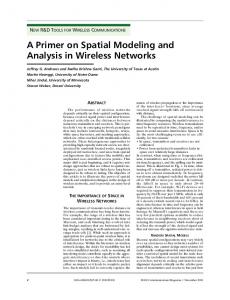
Proposition 1. For λi = σ > 0, i = 1, . . . , n and β = 1, the throughput has the following properties: (i) Symmetric: θi = θn−i+1 , i = 1, 2, . . . , n. (ii) Alternating and converging: (−1)i (θi+1 − θi ) is positive and decreasing for i = 1, 2, . . . , bn/2c. The proof of Proposition 1 is presented in Appendix A. In Figure 1 we see that for nearest-neighbor blocking, the largest difference in throughput is between θ1 and θ2 : The boundary node has a far better position than its direct neighbor. Indeed, as proved in Proposition 1(ii), this is the most unfair situation, and it persists even in larger networks where the node-in-the-middle problem is mitigated by the activity of the remaining nodes. In fact, as the number of nodes becomes large, we have the following result. Proposition 2. As n → ∞, √ 1 + 1 + 4σ θ1 ∼ . θ2 2

(11)

Proof. We have that θ1 ∝ Zn−2 and θ2 ∝ Zn−3 , where Z0 = 1, Z1 = 1 + σ, Zi+1 = Zi + σZi−1 . It immediately follows that (see [12]) X 1 + σx , Zi xi = 1 − x − σx2 i and so 1 Zi ∼ √ 1 + 4σ



1+

√ i+2 1 + 4σ , 2

which gives the result.

Θi

Θi

with the outer nodes having the highest throughput. Moreover, the throughput is symmetric in all figures, and exhibits some form of oscillatory behavior. These observations are formalized in the following result.

0.7

0.6

0.6

0.5

0.5

0.4

0.4

0.3

0.3

0.2

0.2

0.1

We note that for β = 1, alternative descriptions of Zi exist of the forms p 1 Zi = (−σ) 2 (i+1) Ui+1 ( −1/4σ)

0.1 1

2

3

4

5

6

i

1

2

(a) n = 6

3

4

5

6

7

8

9

i

(b) n = 9

Θi 0.7

0.7

0.6

0.6

0.5

0.5

0.4

0.4

0.3

0.3

0.2

0.2

b i+1 c 2

Θi

0.1

Zi =

2

3

4

5

6

7

8

9 10 11 12

i

3

(c) n = 12 Σ = 10

Σ=5

5

7

9

11

13

15

i

(d) n = 15 Σ=2

Σ=1

X j=0

0.1 1

where Un (x) is the nth Chebyshev polynomial of the second kind, and

Σ = 0.5

Σ = 0.2

Σ = 0.1

Figure 1: The per-node throughput for β = 1 and various values of n and σ Figures 1(a)-1(d) show the per-node throughput for various values of n and σ. All figures display a similar pattern,

! i+1−j j σ . j

The latter expression can be interpreted as the summation over all possible combinations of nodes that can be active simultaneously. Figure 1 shows another interesting characteristic of this network. Increasing σ leads in many cases to a higher throughput for each of the nodes. Hence, in such situations, one may want to increase σ further. However, we also observe that there exists a critical value σ ∗ , such that at least one of the throughputs θi decreases as σ increases beyond σ ∗ . The characterization of this critical value is a possible topic for future research. Results similar to those presented in this section can be obtained for β ≥ 2. As an example, Figures 2(a)-2(b) show the per-node throughput for n = 9 and β = 2, 3. Both figures exhibit similar oscillatory behavior as observed for β = 1, although the oscillation period increases with β.

Θi

Θi 0.4

The second special case corresponds to the situation where the number of nodes n equals 2(β + 1), so that a node blocks at least half of the network.

0.5 0.3

0.4 0.3

0.2

0.2 0.1 0.1 1

2

3

4

5

6

7

8

9

i

1

2

3

(a) β = 2 Σ = 10

4

5

6

7

8

9

i

(b) β = 3

Σ=5

Σ=2

Σ=1

Σ = 0.5

Σ = 0.2

Proof. To achieve equal throughputs, we see from (4) and (5) that for the case at hand we should solve the system of equations

Σ = 0.1

Figure 2: The per-node throughput for n = 9 and various values of β and σ

4.

Proposition 4. For tandem networks with n = 2m nodes, m ∈ N, and β = m − 1, setting λi = σ(1 + σ)i−1 for i = 1, . . . , m yields equal throughputs σ , ∀i. (18) θi = 1 + mσ

λ1 + λ1 (λm+1 + · · · + λn ) = λ2 + λ2 (λm+2 + · · · + λn ) = λ3 + λ3 (λm+3 + · · · + λn ) .. . = λm + λm λn .

FAIRNESS

In this section we present a way to completely remove the unfairness observed in Section 3. In order to do so, we choose node-dependent activity rates λi such that all nodes have equal throughput. Hence, we aim for strict fairness of the form θ1 = θ2 = · · · = θn . From (4) and (5) we see that in order to meet this objective we have to solve a system of n nonlinear equations. It appears that in general this system cannot be solved directly. We therefore choose a more indirect approach, for which we first consider two special cases that considerably reduce the complexity of the problem. The first case is where β = n − 2, so that all but the two outer nodes will block the entire network. Proposition 3. For tandem networks with 3 or more nodes, and β = n−2, setting λ1 = λn = σ and λi = σ(1+σ) for all other nodes yields equal throughputs σ , ∀i. (12) θi = 1 + (n − 1)σ Proof. The expression for the throughput in (5) can be written as θ1 = Z −1 λ1 (1 + λn ), θi = Z

−1

λi ,

i = 2, 3, . . . , n − 1,

θn = Z −1 λn (1 + λ1 ).

(15)

The inherent symmetry of the model allows us to set λ1 = λn . Moreover, for the throughput of the other nodes to be equal, we require λ2 = · · · = λn−1 = λ1 (1 + λ1 ). If we set λ1 = σ, and substitute this into (13)-(15), we get a throughput of θi = Z −1 σ(1 + σ).

(16)

The normalization constant Z can be determined by summing over all feasible states: Z =1+

n X

λi + λ1 λn

i=1

= 1 + (n − 2)σ(1 + σ) + 2σ + σ 2 = (1 + σ)(1 + (n − 1)σ).

Indeed, the throughput of node i can be written as a sum over all states in which node i is active. Using symmetry, (19) can be written as λ1 + λ1 (λ1 + · · · + λm ) = λ2 + λ2 (λ1 + · · · + λm−1 ) = λ3 + λ3 (λ1 + · · · + λm−2 ) .. . = λm + λm λ1 .

(17)

Substituting (17) into (16) yields (12). The instance n = 5, β = 3 of Proposition 3 was considered in [2].

(20)

Let λ1 = σ > 0. The solution to (20) reads λi = σ(1 + σ)i−1 ,

i = 1, . . . , m,

and this yields θi = Z −1 σ(1 + σ)m .

(21)

We can obtain Z by summing over all possible states: Z =1+

n X

λi +

i=1

(13) (14)

(19)

=1+

m X i=1

m X i=1

λi +

m X

λi

n X

λj

j=i+m

λi (1 + λ1 + · · · + λm−i−1 )

i=1 m

= 1 + ((1 + σ) − 1) + mσ(1 + σ)m = (1 + mσ)(1 + σ)m .

(22)

Substituting (22) into (21) gives (18). It is clear that the complexity of the system of equations governed by (5) reduces considerably for the choices of β discussed in Propositions 3 and 4. For general β, however, this system remains rather complicated, and the approach taken in the proofs of Propositions 3 and 4 no longer seems to work. This is mainly due to the fact that the equations are nonlinear. Hence, instead of solving the system of equations in a direct fashion, we now take a different approach. First observe that the fair activity rates in Propositions 3 and 4 only depend on the number of neighbors (nodes within distance β) that each node has. Denote by γ(i) the number of neighbors of node i, let σ > 0, and define activity rates λ∗i as in (1). We see that this choice is consistent with the fair activity rates in Propositions 3 and 4. We now show that λ∗i indeed achieves fairness for all β. To this end, we first show

that when the activity rates are chosen according to (1), the recursive relation (6)-(7) for the normalization constant Zi has a closed-form solution.

Substituting (23) into (30) yields min{m,β}

Zn = (1 + σ)n−β +

Lemma 1. Let σ > 0 and choose λ∗ = (λ∗1 , . . . , λ∗n ) as in (1). Then Zi = (1 + σ)i ,

(23)

Proof. This can be verified by substituting the solution (23) into the relations (6) and (7). For i ≤ β + 1, (6) gives Zi = 1 + σ + σ(1 + σ) + · · · + σ(1 + σ)i−1 = (1 + σ)i . For (7) we see that Zi = (1 + σ)i−1 + σ(1 + σ)β (1 + σ)i−β−1 = (1 + σ)i ,

σ(1 + σ)i−1 (1 + σ)n−β−i

i=1

+ i = 1, 2, . . . , n − β.

X

β X

σ(1 + σ)n−β−i

i=m+1

= (1 + σ)n−β−1 (1 + (β + 1)σ).

(31)

Combining (31) and (29) then gives the result. Theorem 2 suggests a combination of efficiency and fairness that is remarkable for this type of multi-access protocol. By varying σ, this protocol can achieve any fair per-node throughput up to 1/(1 + β), which is the highest possible throughput.

covering the case i ≥ β + 2. With Lemma 1 we are now in the position to prove our main result. Theorem 2. Let σ > 0 and choose λ∗ as in (1). Then σ . (24) θi (λ∗ ) = 1 + (1 + β)σ Proof. To prove this result we substitute the normalization constants from Lemma 1 into the expression for the throughput in (8). We distinguish between different values of i. For i ≥ β + 1 and i ≤ n − β we see that λ∗i = σ(1 + σ)β and Zi−β−1 = (1 + σ)i−β−1 , Zn−i−β = (1 + σ)n−i−β .

(25)

Similarly for i ≥ β + 1 and i ≥ n − β + 1 we have λ∗i = σ(1 + σ)n−i and Zi−β−1 = (1 + σ)i−β−1 , Zn−i−β = 1.

(26)

For i ≤ β and i ≤ n − β we have λ∗i = σ(1 + σ)i−1 , and Zi−β−1 = 1, Zn−i−β = (1 + σ)n−i−β ,

(27)

and finally for i ≤ β and i ≥ n − β + 1 we have λ∗i = σ(1 + σ)n−β−1 and Zi−β−1 = 1, Zn−i−β = 1.

(28)

Substituting (25)-(28) into (8) yields θi = Zn−1 σ(1 + σ)n−β−1 .

(29)

We next consider the normalization constant. Choose m such that n = β + m. Then Zn = Zn−1 + λ∗n Zn−β−1 = Zn−2 + λ∗n−1 Zn−β−2 + λ∗n Zn−β−1 .. . = Zn−β +

β X i=1

λ∗n+1−i Zn−β−i .

(30)

5.

CONCLUSIONS AND OUTLOOK

In this paper we studied the unfairness in tandem multiaccess networks. Under the assumption that all nodes have the same activity rates, we obtained some structural properties of the network. We then proposed node-dependent activity rates as a function of the number of neighbors, and showed that these rates provide equal throughput for all nodes. The fair activity rates found in (1) increase with the number of neighbors. Intuitively, this structure can be explained by the observation that, as the number of neighbors increases, a node requires a higher activity rate to retain its throughput. Consequently, the rule in (1), which is exact in tandem networks, might serve as a heuristic in more complex networks. The performance of such a heuristic can be easily tested, and is an interesting topic for further research. Finding activity rates that provide strict fairness for networks beyond the tandem network is challenging. Kelly [8] obtained results for trees with nearest-neighbor blocking, and finds that rates such as in (1), where nodes on the leafs of the tree have lower rates than those in the center, provide strict fairness. For such trees, it seems possible to extend Kelly’s result to the β-hop blocking situation. Finally, let us mention that regular networks like grids or trees may not always be a good representation of topologies encountered in practice, which in general are less structured. The results obtained in this paper however rely heavily on the diagonal structure of the capacity matrix A in (3), which will no longer exist for more irregular networks. However, also for more general networks, and hence more general matrices A, the objective of equal througputs boils down to solving the system of nonlinear equations that follows from (5). In fact, (5) can be described in terms of the the mapping (with λ = (λ1 , . . . , λn ) ∈ (0, ∞)n ) ! n X Y ωi λ 7→ θ(λ) = Z · X · Π = λi ω∈Ω i=1 ωk 6=0

k=1,...,n

with θ(λ) ∈ (0, ∞)n . It can be shown that the mapping θ is globally invertible on (0, ∞)n . Thus, given a vector c ∈ (0, ∞)n , there is a unique λ = λ(c) ∈ (0, ∞)n such that θ(λ) = c. When c has identical entries, this corresponds to all nodes having equal throughput. The full analysis of this fixed-point equation is rather involved and will appear elsewhere.

APPENDIX A.

Proposition 1(ii) follows from (−1)i (θi+1 − θi )   X = (−1)i θi+1 − Z −1 a(i, l, n)σ l

PROOF OF PROPOSITION 1

We first establish an auxiliary result. Define a(i, l, n) as the number of states in which exactly l nodes are active, including node i. For successive nodes, the following relation holds.

l

 X = (−1)i θi+1 − Z −1 (a(i, l − 1, n − 2) l

Lemma 2. Let n ∈ N, i ≤

n 2

l

+ a(i, l, n − 1))σ  X > (−1)i θi+1 − Z −1 (a(i, l − 1, n − 2)

− 1. Then:

a(i, l, n) = a(i + 1, l, n),

l ≤ i,

(32)

a(i, l, n) > a(i + 1, l, n), a(i, l, n) < a(i + 1, l, n),

i odd, i < l ≤ dn/2e , i even, i < l ≤ dn/2e .

(33) (34)

l

 + a(i + 1, l, n − 1))σ l   X = (−1)i θi+1 − Z −1 a(i + 2, l, n)σ l

Proof. The proof is by induction on i. Conditioning on activity of node 1 and node n yields the following relations: a(i, l, n) = a(i − 2, l − 1, n − 2) + a(i − 1, l, n − 1),

(35)

a(i, l, n) = a(i, l − 1, n − 2) + a(i, l, n − 1).

(36)

a(0, l, n) = 0 for all n and l; a(1, l, n) = 1 for l > 0 and all n; a(1, l, n) = 0 for l ≤ 0 and all n. Hence, the initialization step of the induction is a(0, l, n) < a(1, l, n), a(0, l, n) = a(1, l, n),

0 < l < dn/2e , l ≤ 0.

Consider odd i ≤ dn/2e − 2, let i + 1 < l < dn/2e, and assume a(i, l, n) > a(i + 1, l, n). Using (35) and (36) we get a(i + 1, l, n) = a(i + 1, l − 1, n − 2) + a(i + 1, l, n − 1) < a(i, l − 1, n − 2) + a(i + 1, l, n − 1) = a(i + 2, l, n). This proves assertion (33). Assertions (32) and (34) can be proved in a similar manner. We now use Lemma 2 to prove Proposition 1. Proof. (Proposition 1) (i) This can be shown by rewriting the throughput as follows: X a(i, l, n)σ l θi = Z −1 l

= Z −1

X

a(n − i + 1, l, n)σ l = θn−i+1 .

l

(ii) First, we show that (−1)i (θi+1 − θi ) is positive. That is, (−1)i (θi+1 − θi ) X = (−1)i Z −1 (a(i + 1, l, n) − a(i, l, n)) σ l l bn/2c

= (−1)i Z −1

X

(a(i + 1, l, n) − a(i, l, n)) σ l > 0,

l

= (−1)i+1 (θi+2 − θi+1 ). This completes the proof.

B.

The boundary conditions are readily found as

(37)

l=i+1

where the inequality follows from Lemma 2. Using (37),



REFERENCES

[1] R. Boorstyn and A. Kershenbaum. Throughput analysis of multihop packet radio. In Proc. of ICC, pages 1361–1366, 1980. [2] D. Denteneer, S. Borst, P. Van de Ven, and G. Hiertz. IEEE 802.11s and the philosophers’ problem. Statistica Neerlandica, 62(3):283–298, 2008. [3] M. Durvy, O. Dousse, and P. Thiran. Modeling the 802.11 protocol under different capture and sensing capabilities. In Proc. of INFOCOM, pages 2356–2360, 2007. [4] M. Durvy, O. Dousse, and P. Thiran. Self-organization properties of CSMA/CA systems and their consequences on fairness. IEEE Transactions on Information Theory, to appear. [5] M. Garetto, T. Salonidis, and E. Knightly. Modeling per-flow throughput and capturing starvation in CSMA multi-hop wireless networks. In Proc. of INFOCOM, pages 1–13, 2006. [6] G. Hiertz, Y. Zang, S. Max, T. Junge, E. Wei, D. Denteneer, L. Berlemann, and S. Mangold. IEEE 802.11s - WLAN mesh standardization and high performance extensions. IEEE Network, 22(3):12–19, 2008. [7] L. Jiang and J. Walrand. A distributed CSMA algorithm for throughput and utility maximization in wireless networks. In Proc. of Allerton conference on communication, control, and computing, pages 1511–1519, 2008. [8] F. Kelly. Stochastic models of computer communication systems. Journal of the Royal Statistical Society. Series B, 47(3):379–395, 1985. [9] F. Kelly. Loss networks. The Annals of Applied Probability, 1(3):319–378, 1991. [10] L. Kleinrock and F. Tobagi. Packet switching in radio channels: part I - carrier sense multiple-access modes and their throughput-delay characteristics. IEEE Transactions on Communications, 23(12):1400–1416, 1975. [11] J. Liu, Y. Yi, A. Prouti`ere, M. Chiang, and H. Poor. Convergence and tradeoff of utility-optimal CSMA. http://arxiv.org/abs/0902.1996 (preprint), 2009.

[12] E. Pinsky and Y. Yemini. The asymptotic analysis of some packet radio networks. IEEE Journal on Selected Areas in Communications, 4(6):938–945, 1986. [13] S. Rajagopalan and D. Shah. Distributed algorithm and reversible network. In Proc. of CISS, pages 498–502, 2008. [14] A. Vasan, R. Ramjee, and T. Woo. ECHOS Enhanced capacity 802.11 hot spots. In Proc. of INFOCOM, pages 1562–1572, 2005. [15] X. Wang and K. Kar. Throughput modelling and fairness issues in CSMA/CA based ad-hoc networks. In Proc. of INFOCOM, pages 23–34, 2005. [16] X. Yang and N. Vaidya. On physical carrier sensing in wireless ad hoc networks. In Proc. of INFOCOM, pages 2525–2535, 2005. [17] J. Zhu, X. Guo, L. Yang, and W. S. Conner. Leveraging spatial reuse in 802.11 mesh networks with enhanced physical carrier sensing. In Proc. of ICC, pages 4004–4011, 2004.