in partial fulfillment of the requirements for the degree of. MASTER OF SCIENCE. Major: Computer Science. Major Professor: Vasant ... 3.2.2 Angular distance based measurements . .... hippocampal formation in rodent spatial learning [ON78].
Spatial learning and localization in rodents: Behavioral simulations and results by Rushi Prafull Bhatt
A thesis submitted to the graduate faculty in partial ful llment of the requirements for the degree of MASTER OF SCIENCE
Major: Computer Science Major Professor: Vasant Honavar
Iowa State University Ames, Iowa 2000 c Rushi Prafull Bhatt, 2000. All rights reserved. Copyright
ii
Graduate College Iowa State University
This is to certify that the Master's thesis of Rushi Prafull Bhatt has met the thesis requirements of Iowa State University
Major Professor For the Major Program For the Graduate College
iii
TABLE OF CONTENTS CHAPTER 1. OVERVIEW . . . . . . . . . . . . . . . . . . . . . . . . . . . .
1
1.1 Introduction . . . . . . . . . . . . . . . . . . . . . . . . . . . . . . . . . . . . . .
1
1.2 Organization of Thesis . . . . . . . . . . . . . . . . . . . . . . . . . . . . . . . .
2
CHAPTER 2. REVIEW OF FUNCTIONAL AND ANATOMICAL ORGANIZATION OF THE HIPPOCAMPAL FORMATION . . . . . . . .
3
2.1 Introduction . . . . . . . . . . . . . . . . . . . . . . . . . . . . . . . . . . . . . .
3
2.2 Inputs and Outputs in the Rodent Hippocampal Formation . . . . . . . . . . .
4
2.2.1 Inputs to the hippocampal formation . . . . . . . . . . . . . . . . . . . .
5
2.2.2 Outputs from the hippocampal formation . . . . . . . . . . . . . . . . .
6
2.3 Anatomy of the Hippocampal Formation . . . . . . . . . . . . . . . . . . . . . .
6
2.3.1 Entorhinal cortex and the perforant path . . . . . . . . . . . . . . . . .
7
2.3.2 Dentate gyrus and mossy bers . . . . . . . . . . . . . . . . . . . . . . .
8
2.3.3 CA3-CA1 connections . . . . . . . . . . . . . . . . . . . . . . . . . . . .
8
2.4 Physiological Properties of Hippocampal Cells . . . . . . . . . . . . . . . . . . .
11
2.4.1 Spatiality and directionality of pyramidal cell ring in area CA . . . . .
11
2.4.2 Spike characteristics of hippocampal place cells . . . . . . . . . . . . . .
13
2.5 Conclusion . . . . . . . . . . . . . . . . . . . . . . . . . . . . . . . . . . . . . .
14
CHAPTER 3. SPATIAL LEARNING FROM A COMPUTATIONAL CONTEXT . . . . . . . . . . . . . . . . . . . . . . . . . . . . . . . . . . . . .
16
3.1 Background . . . . . . . . . . . . . . . . . . . . . . . . . . . . . . . . . . . . . .
16
3.2 Sensory Information Available to a Mobile Robot or a Navigating Animal . . .
18
3.2.1 Linear distance based measurements . . . . . . . . . . . . . . . . . . . .
18
iv 3.2.2 Angular distance based measurements . . . . . . . . . . . . . . . . . . .
19
3.3 Representation of Information . . . . . . . . . . . . . . . . . . . . . . . . . . . .
20
3.3.1 Storage . . . . . . . . . . . . . . . . . . . . . . . . . . . . . . . . . . . .
20
3.3.2 Retrieval . . . . . . . . . . . . . . . . . . . . . . . . . . . . . . . . . . .
21
3.3.3 Noise and inaccuracies in sensors and path integrator . . . . . . . . . .
21
3.4 Conclusion . . . . . . . . . . . . . . . . . . . . . . . . . . . . . . . . . . . . . .
22
CHAPTER 4. FORMALIZATION OF COGNITIVE MAPS FOR SPATIAL LEARNING AND NAVIGATION . . . . . . . . . . . . . . . . . . .
24
4.1 Preliminaries . . . . . . . . . . . . . . . . . . . . . . . . . . . . . . . . . . . . .
24
4.1.1 The local view . . . . . . . . . . . . . . . . . . . . . . . . . . . . . . . .
25
4.1.2 The PI state . . . . . . . . . . . . . . . . . . . . . . . . . . . . . . . . .
28
4.1.3 The cognitive map . . . . . . . . . . . . . . . . . . . . . . . . . . . . . .
31
4.2 Intra Map Operations . . . . . . . . . . . . . . . . . . . . . . . . . . . . . . . .
32
4.2.1 Operations on LV . . . . . . . . . . . . . . . . . . . . . . . . . . . . . .
32
4.2.2 Operations on PI . . . . . . . . . . . . . . . . . . . . . . . . . . . . . . .
34
4.3 Inter-Map Operations . . . . . . . . . . . . . . . . . . . . . . . . . . . . . . . .
35
4.3.1 Choosing a context . . . . . . . . . . . . . . . . . . . . . . . . . . . . . .
35
4.3.2 Learning the context . . . . . . . . . . . . . . . . . . . . . . . . . . . . .
37
4.3.3 Merging environment contexts . . . . . . . . . . . . . . . . . . . . . . .
38
4.4 Selection of Actions . . . . . . . . . . . . . . . . . . . . . . . . . . . . . . . . .
39
CHAPTER 5. EXISTING COMPUTATIONAL MODELS . . . . . . . . .
40
5.1 Place-Response Based Navigation Models . . . . . . . . . . . . . . . . . . . . .
40
5.2 Topological Navigation Models . . . . . . . . . . . . . . . . . . . . . . . . . . .
41
5.3 Metric Based Navigation Models . . . . . . . . . . . . . . . . . . . . . . . . . .
42
CHAPTER 6. COMPUTATIONAL MODEL FOR RODENT SPATIAL NAVIGATION AND LOCALIZATION . . . . . . . . . . . . . . . . . . . .
45
6.1 The Basic Computational Model . . . . . . . . . . . . . . . . . . . . . . . . . .
45
v 6.2 Learning and Updating Goal Locations . . . . . . . . . . . . . . . . . . . . . . .
49
6.2.1 Representing multiple goals . . . . . . . . . . . . . . . . . . . . . . . . .
50
6.2.2 Navigating to goals . . . . . . . . . . . . . . . . . . . . . . . . . . . . . .
51
6.3 Merging Di�erent Learning Episodes (frame merging) . . . . . . . . . . . . . .
52
CHAPTER 7. BEHAVIORAL EXPERIMENTS AND RESULTS
....
53
7.1 Experiments of Collett et al. (1986) . . . . . . . . . . . . . . . . . . . . . . . .
53
7.2 Water-Maze Experiments of Morris (1981) . . . . . . . . . . . . . . . . . . . . .
56
7.3 Discussion . . . . . . . . . . . . . . . . . . . . . . . . . . . . . . . . . . . . . . .
58
7.4 Variable Tuning Widths of EC Layer Spatial Filters . . . . . . . . . . . . . . .
60
7.5 All-Or-None Connections Between EC and CA3 Layers . . . . . . . . . . . . . .
61
7.6 Association of Rewards With Places . . . . . . . . . . . . . . . . . . . . . . . .
62
7.7 Simulation Results . . . . . . . . . . . . . . . . . . . . . . . . . . . . . . . . . .
64
7.8 Firing Characteristics of Units . . . . . . . . . . . . . . . . . . . . . . . . . . .
64
7.9 Landmark Prominence Based on Location and Uniqueness . . . . . . . . . . . .
66
CHAPTER 8. CONCLUSIONS . . . . . . . . . . . . . . . . . . . . . . . . .
68
BIBLIOGRAPHY . . . . . . . . . . . . . . . . . . . . . . . . . . . . . . . . . . .
71
1
CHAPTER 1. OVERVIEW
1.1 Introduction The computational strategies used by animals to acquire and use spatial knowledge for navigation have long been the subject of study in Neuroscience, Cognitive Science, and related areas. A vast body of data from lesion studies and cellular recordings directly implicates the hippocampal formation in rodent spatial learning [ON78]. The present model is based on the anatomy and physiology of the rodent hippocampus [She74, CS92]. We draw inspiration from the locale hypothesis, which argues for the association of con gurations of landmarks in the scene to the animal's own position estimates at di�erent places in the environment [ON78]. The system that generates the animal's own position estimate using the vestibular as well as motor commands issued is referred to as the Path Integration (PI) system [ON78]. The PI is hypothesized to play an important role in spatial tasks in terms of disambiguation of con icting spatial cues and generation of relational information between available landmarks. At the same time, PI system is an important component of route based navigation system as it can supply place labels to incoming sensory cues which can be e�ectively used to compute the sequence of actions that can be used to guide the animal to a goal. From Various lesion studies it has been found that the hippocampus plays an important role in spatial tasks, that is, tasks that involve speci c locations and geometric relationships between objects. Lesions to hippocampus in rodents produce a severe de cit in learning of new spatial tasks, while at the same time keeping the stimulus-response type of task learning largely intact [MGRO82, MW93a, DMW99]. Apart from its linkage with the spatial tasks, it has been found that the hippocampus plays an important role in incorporation and retention of new memories. It has been proposed
2 by numerous researchers that the hippocampus works as a temporary storage for new memories [Mar71, Buz89, CE93]. These memories are then supposed to be transferred to a more permanent storage site. This idea is still under scrutiny by many researchers and is not completely accepted. Opponents of this transfer of memory idea hypothesize that the hippocampus works more like an index for retrieval of memories and is not simply a temporary storage site [NM97, ESYB96, Eic96]. Despite such great interest in spatial learning and the hippocampal formation, there are relatively few computational or conceptual models that explain this wealth of experimental data at a low level, and yet be general enough to shed new light on the general principles that guide learning and behavior. By low level we mean a level at which the performance of the hippocampal system is explained with respect to its performance on speci c tasks and the degradation of performance on the same tasks upon lesion or inhibition of the hippocampus. In this thesis, we examine how the computational model developed by Balakrishnan and Honavar (1999) [Bal99] explains some of the important experiments on the rodent spatial learning and navigation system which critically involves the hippocampus and its surrounding brain regions.
1.2 Organization of Thesis The next chapter presents an overview of the anatmoical and functional characteristics of the hippocampal formation. Chapter 5 discusses some existing models for explaining the function of the hippocampus. In Chapter 6 we discuss the computational model for rodent spatial learning and navigation developed by Balakrishnan and Bousquet, and Honavar[BBH98d]. This model has been utilized in the present thesis to perform some behavioral experiments that validate the model in the context of reproducibility of rodent behavior. These experiments will be discussed in Chapter 7. We then reach the main conclusions of this thesis and propose some related future work in Chapter 8.
3
CHAPTER 2. REVIEW OF FUNCTIONAL AND ANATOMICAL ORGANIZATION OF THE HIPPOCAMPAL FORMATION
2.1 Introduction The hippocampal formation consists of the hippocampus proper (also called \Ammon's Horn", abbreviated as CA) and surrounding structures; dentate gyrus and subiculum. The hippocampus is a bi-lateral limbic structure, the details of which will be discussed in the following sections. The hippocampal formation is believed to be one of the major sites responsible for processing and incorporation of new spatial information [ON78]. One of the reasons to believe so is based on lesion studies carried out on animals, where it was found that animals with lesions in the hippocampal region were unable to learn spatial tasks [ON78, MGRO82]. Similar ndings are also available in human subjects. A famous example is that of patient H.M. who, after undergoing bilateral resection of temporal lobes was rendered completely unable to learn and remember information. At the same time H.M. had a normal short-term memory and was able to recall many events that happened before the surgery [Mil72, Mil73]. Further, it was also found that H.M. was able to learn new motor skills but he was unaware of his coming across the task before. Another case that attracted much attention was that of patient R.B.. Patient R.B. was found to be unable to learn and remember new information. On the other hand, he showed normal conditioning, priming behavior. After the death of R.B. due to unrelated causes, it was found that the degeneration was mainly con ned to the CA1 region of the hippocampus [ZMSA86]. The role played by the hippocampus in human navigation is still a matter of controversy.
4 Recent studies using positron emission tomography (PET) scan and regional cerebral blood
ow (rCBF) has shown that speci c subparts of the human hippocampus are active when subjects perform navigational tasks. The measurements were made while human subjects played a virtual reality game (Duke Nukem 3D) and it was found that the activity in the right hippocampus was proportionate to the accuracy of navigation. Activity level in the left hippocampus did not co-vary much with the accuracy of navigation, and it was interpreted that this region actively maintains the memory trace of the destination during navigation of recollection of paths taken during previous trials [MBD+ 98]. Although the foregoing study precisely states the brain regions active during spatial navigation and planning, the role of human hippocampus during spatial tasks involving physical locomotion are still unclear. More recent studies in primates have shown existence of \Spatial view" cells in the primate hippocampus. Recordings from the monkey hippocampus were performed while the monkey walked actively in an obstacle-free laboratory room. The cells rings were found to have a high correlation with which area of the environment, in this case laboratory walls, the monkey was looking at. This characteristic is in contrast with the rodent hippocampus where the pyramidal cells re when rodent is at a particular place in its environment regardless of its orientation [RTR+ 98]. Previous studies by the same group have shown that 9.3% of neurons in primate hippocampus respond to stimuli appearing at some but not other corners of a computer monitor. 2.4% of cells only red when a novel stimulus at speci c locations on the computer monitor were displayed for the monkey [RMC+ 89]. Furthermore, it has been shown that these Spatial view cells encode location of stimuli with reference to an allocentric frame and not the position of stimulus on the retina, head direction or the location of the monkey [GFRR99].
2.2 Inputs and Outputs in the Rodent Hippocampal Formation The hippocampal formation receives highly processed sensory information from the cortical regions via the entorhinal cortex and from non-cortical regions via the fornix. It also projects back to the cortical regions via the entorhinal cortex and to the subcortical regions via fornix, as will be discussed shortly.
5
2.2.1 Inputs to the hippocampal formation The inputs to the hippocampal formation can be further divided into those from the cortical regions and those from the non-cortical regions. The inputs from the cortical regions come via projections onto the entorhinal cortex which in turn projects to the hippocampal formation. Tract tracing experiments have shown major pathways originating from the inferior temporal gyri (higher processing area for visual sensory information), parietal and temporal lobes (higher processing area for auditory sensory information) and also from the frontal lobes. The only exception here is the olfactory information. Direct projections, as opposed to projections from higher areas of sensory information processing in the cortex, from the olfactory bulb and pyriform cortex onto entorhinal cortex have been found. Most inputs from these cortical regions arrive into the super cial cortical layers of the entorhinal cortex. Entorhinal cortex is thus believed to be a place for multi-sensory information integration. It has been contended that the hippocampal formation receives inputs form virtually all higher cortical regions [CE93]. The entorhinal cortex also receives inputs from amygdala, medial septum, dorsal raphe nucleus, locus ceruleus and parts of the thalamus. Most of the pathways from the septum onto hippocampus are cholinergic as well as GABAergic [TM91]. A recent study has found select nuclear divisions of the amygdala project to the entorhinal cortex as well as hippocampus, subiculum and parasubiculum in a topographically ordered fashion [PRS+99]. A coarse topographic speci city in terms of projections from other cortical as well as non cortical areas has also been observed. More rostral cortical areas project more heavily to more rostral portions of the parahippocampal cortex, and more caudal neocortical areas project more heavily to more caudal portions of the parahippocampal cortex [CE93]. The inputs from the non cortical structures come via the fornix. The fornix carries inputs from the thalamus, septum, hypothalamus and other brainstem nuclei. The subcortical inputs are believed to serve as modulatory signals that in uence activity in the hippocampal formation [TM91]. Most of the inputs to the hippocampal formation are believed to be excitatory, except some
6 inputs from the septum, as mentioned above. Apart from that, the hippocampus receives connections from the other hippocampus through the commissural pathways that join the two hippocampi across the midline [CS92].It is reasonable to assume that cortical inputs carry time-dependent information arriving from the external events noted by the sensory systems [TM91].
2.2.2 Outputs from the hippocampal formation The entorhinal cortex also projects back to the same cortical areas mentioned above. Most of the projections from entorhinal cortex to the cortical regions have been observed to be from cortical layers V/VI. Entorhinal cortex also sends bers back to the septum. Projections to the septum also originate from the pyramidal cells in the hippocampus as well as from non pyramidal cells from the same area. The pyramidal cells of CA3 and CA1 subdivisions of CA project to the lateral septum. These connections are excitatory. The non-pyramidal cells in the hippocampus project to the medial septum/diagonal band. The latter projections are believed to be inhibitory [TM91].
2.3 Anatomy of the Hippocampal Formation The anatomical connections in the hippocampal formation are some of the most wellstudied, partly due to the systematic structure in the connections themselves, and partly because of the numerous examples of neuronal plasticity that have been observed in this region. The hippocampus is an elongated C shaped structure spanning from the septal nuclei to the temporal cortex. Figure 2.1 shows major synaptic connections found in slices taken perpendicular to to the long axis (septotemporal axis). These slices show a structure that resembles two interlocking `C' shaped arrangements. One `C' is known as the Dentate gyrus, within which the granule cell layer is the principle layer. The other `C' is the hippocampus proper, and is also referred to Cornu Ammonis (abbreviated as CA) and is subdivided into regions CA1 through CA4. Such a structure is seen all along the septotemporal axis.
7
Figure 2.1 Schematic of connections in hippocampus Using simultaneous stimulation and recording studies as well as neuronal tract tracing techniques, the major connection pathways in hippocampal formation are now well-understood [AW89]. In brief, the circuitry can be described as follows.
2.3.1 Entorhinal cortex and the perforant path The entorhinal cortex is the origin of a strong projection (the perforant pathway) to the dentate gyrus and hippocampus [AW89]. Cortical layers II and III of the entorhinal cortex project via perforant path bers into the dentate gyrus, the hippocampus and the molecular layer of the subiculum. Anterograde and retrograde tracing techniques have shown that projections from very constrained regions in the entorhinal cortex reach wide septotemporal areas of the dentate gyrus, as opposed to earlier suggestions by Andersen, Bliss and Skerde (1972) . It can also be concluded that a single layer of the dentate gyrus along the septotemporal axis is innervated by multiple focal points in the entorhinal cortex. One of the suggestions for the functional role is that these highly divergent connections result in a sparse, distributed encoding of the highly processed sensory information which is then delivered to the hippocampus via the dentate gyrus. It should also be noted here that far reaching projections of the inhibitory 'basket cells' in the dentate gyrus have also been found [SDL78]. It can therefore be concluded that excitatory as well as inhibitory connections span over long distances over the septotemporal axis in the
8 hippocampus.
2.3.2 Dentate gyrus and mossy bers The dentate gyrus receives projections from the entorhinal cortex through the perforant path. Dentate gyrus in turn provides input to the CA3 layer of the hippocampus proper. \The dentate gyrus can be divided into three layers: The molecular layer, in which perforant path bers terminate; the granule cell layer, which is populated by the principal cell type, the granule cell; and a deep or polymorphic layer which is populated by a variety of neuronal types. The granule cells give rise to the mossy bers, which collateralize in the polymorphic layer and then enter the CA3 layer where they form en passant synapses with the proximal dendrites of the pyramidal cells" [AW89]. These mossy ber synapses with CA3 are strong, which has led researchers to suggest that they provide the context [O'K89] or reference frame of the task to be performed [MBG+ 96], by transformation of the sensory input activity arriving at entorhinal cortex into a non-overlapping activity pattern of granule cells, which in turn are conveyed to the pyramidal cells in the CA3 layer. It has been found that on an average, CA3 pyramidal cells get about 330,000 contacts from the mossy bers collectively, or, a granule cell makes contact with around 14 CA3 pyramidal cells and each CA3 pyramidal cell is innervated by only about 46 granule cells [CS92].
2.3.3 CA3-CA1 connections The hippocampus proper can be further divided into stratum moleculare, stratum radiatum, stratum of pyramidal cell bodies and stratum oriens as one progresses further from the septotemporal axis radially. The CA3 region of the hippocampus primarily contains pyramidal cells that show a characteristic complex spiking behavior. These pyramidal cells are arranged in a single layer, in stratum of the pyramidal cell bodies. The dendrites of these cells descend into the deeper stratum oriens as well as into stratum radiatum and stratum lacunosum-moleculare. The CA3 and CA1 pyramidal cells receive inputs from three di�erent sources: (i) from
9 cortical layer II of entorhinal cortex through the perforant path, synapses of which are formed in the uppermost parts of the apical dendrites of pyramidal cells in CA3. Some direct connections from cortical layer III of entorhinal cortex to CA1 apical dendrites have also been found. (ii) from dentate gyrus through mossy bers which make connections to the proximal apical dendrites of CA3 pyramidal cells, and (iii) recurrent inputs from other CA3 pyramidal cells. See Figure 2.2 for a clear picture of the connections mentioned above. Unlike CA3 cells, CA1 cells do not project to other pyramidal cells of CA1 [CS92]. Recurrent collaterals
Entorhinal Cortex (EC) II
Hippocampus Perforant path
III Dg V VI
CA3
Mossy fibers
CA1
Dentate Gyrus
postSub preSub
Olfactory Frontal Parietal Temporal Cortex
Schaffer collaterals
Back projections to cortical areas and septum
Sb Subiculum
Figure 2.2 Schematic of major connection pathways in hippocampus The number of recurrent collaterals on a CA3 pyramidal cell from other CA3 pyramidal cells is believed to be around 6000, or about 1.8% of the CA3 cell population. These recurrent connections are located on the dendritic tree spaced between the mossy and perforant inputs [CS92]. Some researchers have likened the structure of the recurrent collaterals to an auto-associative recurrent network suggesting that CA3 serves as a pattern completion device capable of recalling entire scenes from partially observed data [Mar71, Rol90]. However, others have suggested a hetero-association role, suggesting that these collaterals predict future activations of the neurons based on the current activations [McN89, MN89]. Some experimental evidence for this latter view is provided by [SM96]. In CA3, mossy bers from the dentate gyrus project into a region just above the pyramidal cell layer. Axons from CA3 pyramidal cells then make highly collateralized connections that terminate within the CA3 layer and make strong projections into the CA1 layer via the Scha�er
10 collaterals. As discussed earlier, the CA1 pyramidal cells receive excitatory inputs from the entorhinal cortex via the perforant path and from the CA3 pyramidal cells through the Scha�er collaterals. Axons from the CA1 pyramidal neurons project via the alveus to the subiculum and also to the deep cortical layers of the entorhinal cortex. Subiculum also receives input from the entorhinal cortex and projects to the pre- and post-subiculum, the deep layers of the entorhinal cortex, and to the hypothalamus, septum, anterior thalamus and the cingulate cortex. All these connections are excitatory [CS92]. The a�erents from brain-stem areas to the hippocampus proper have been found to synapse mostly in stratum lacunosum/moleculare of CA1 and CA3 and in a restricted part of the hilar zone under the granule cells in the dentate gyrus. These connections are believed to contribute towards most of the serotonin found in hippocampus [ON78]. It has also been found that for the CA3 pyramidal cells, majority of dendrites were located in stratum oriens, while almost the same amount of dendrites were present in stratum radiatum and stratum lacunosum-moleculare. For the CA1 region pyramidal cells, majority of dendrites were found in stratum radiatum. Presumably, more dendrites in a particular stratum would mean a greater number of en passant synapses as well as synapses with interneurons in the stratum in question [AW89]. CA3 and CA1 regions also contain interneurons that suppress the activity in pyramidal cells. It has been found that the pyramidal cells make excitatory connections to the basket cells present in the stratum of pyramidal cells, which in turn provide GABAergic inhibitory input back to the pyramidal cell. It has been found by experiments with CA1 cells that when Scha�er collaterals and commissural axons in stratum radiatum were stimulated, the range of frequencies under which LTP was produced increased in the presence of a GABA type A receptor agonist (muscimol), while LTP was induced only at very low frequencies in presence of GABA type A antagonist (picrotoxin) [SM99]. Thus, this inhibitory loop, presumably between pyramidal and basket cells is believed to be a controlling mechanism for LTP and LTD induction.
11 It has also been found that interneurons in the lacunosum-moleculare region of CA1 are not restricted to the CA1 region. The dendritic and axonal processes of some of these interneurons were seen ascending in stratum lacunosum-moleculare, crossing the hippocampal ssure, and coursing in stratum moleculare of the dentate gyrus. Stimulation of hippocampal a�erents caused excitatory as well as inhibitory postsynaptic potentials in these interneurons. EPSPs were most e�ectively elicited by stimulation of ber pathways in transverse slices, whereas IPSPs were predominantly evoked when major pathways were stimulated in longitudinal slices. Thus, these interneurons are di�erent in characteristics from the interneurons (for example, basket cells) and the pyramidal cells [LS88a, LS88b]. It has recently been found that during rhythmic oscillations in area CA3, interneurons with similar dendritic and axonal arbors behave di�erently. One group of interneurons is powerfully excited by CA3 pyramidal cells, whereas two other interneuron groups were relatively unaffected by pyramidal cell ring. One of these groups of interneurons is inhibited by other local interneurons during the pyramidal cell bursts. Thus, morphologically similar interneurons are wired radically di�erently and hence produce very dissimilar ring characteristics [MWK98]. It has also been found that one group of these interneurons can undergo LTP while another group is incapable of undergoing LTP. mGluR system is supposed to govern this kind of behavior [Informal talk by Lacaille] The major connections in the hippocampus can be summarized as shown in Figure 2.2 [BBH98a].
2.4 Physiological Properties of Hippocampal Cells 2.4.1 Spatiality and directionality of pyramidal cell ring in area CA Apart from evidence from lesion studies, cellular recordings from pyramidal cells in the hippocampal formation of behaving rodents have show that many such cells re in complex spike bursts only when the animal is in a constrained region of its environment. Such cells show a characteristic, complex spiking behavior which is distinct from other cells found in the vicinity of these cells. O'Keefe named them place cells and the corresponding regions where each is active, the place eld [O'K76]. The speci c regions in which these cells re are well de ned for
12 a given environment and can be manipulated by changing the size and sensory cues available in the environment within which the experiments are carried out [ON78, OD71, TSE97]. Cells with such location-speci c ring have been found in almost every major region of the hippocampal system, including the entorhinal cortex [QMKR92], the dentate gyrus [JM93], hippocampus proper [OD71, O'K76], the subiculum [BMM+ 90, SG94], and the postsubiculum [Sha96]. In addition to place cells, head-direction cells have also been discovered. These cells respond to particular directions of the animal's head, irrespective of its location in the environment. Each such cell res only when the animal's head faces one particular direction (over an approximately 90 degree range) in the horizontal plane. The ring of these cells can be altered by a complex interaction between visual and angular motion signals. Importantly, in every case reported to date, any manipulation that alters the reference direction of one of these cells results in a corresponding alteration in the reference direction for the whole system which is in contrast to hippocampal place cells where partial re-mapping of groups of cells encoding the same environment is possible. These cells were rst discovered in the postsubicular area of the hippocampal formation [Ran84, TMR90a, TMR90b]. Since then, such directional cells have also been discovered in the retrosplenial cortex [CLBM94, CLG+ 94], the anterior thalamus [Tau95, BS95a], and the laterodorsal thalamus [MW93b]. A number of experiments have been performed in order to determine the properties of the place and head-direction cells. It is now known that the spatial representation in the place cells is not grid-like, i.e., adjacent neurons are as likely to represent distant portions of the environment as close ones [O'K76, MKR87, OS87, O'K89, WM93]. Also, place cells are active in multiple places in the environment [OS87] and also in multiple environments [KR83, MKR87, MK87]. Further, places appear to be represented in the hippocampus using an ensemble code, i.e., a set of place cells appear to code for a place [WM93]. Experiments have also revealed that when the animal is introduced into a familiar environment, place elds are initialized based on visual cues and landmarks [MK87, MKR87, SKM90]. Once initialized, the place elds have been found to persist even if the visual cues are removed
13 in the animal's presence [OS87], implying that place cell ring must also be maintained by a source other than visual stimulus. It has been found that place elds of CA1 cells are conserved in darkness, provided the animal is rst allowed some exploration of the apparatus under illuminated conditions [MLC89, QMK90]. This has led to the hypothesis that place elds are maintained by ideothetic (self-motion) mechanisms, i.e., by the path integration system.
2.4.2 Spike characteristics of hippocampal place cells It has been found that the place cells show a very characteristic ring pattern within the ring eld. These cells re in bursts that last for a maximum of 2 seconds and re at a peak rate of around 20 action potentials. Further each burst contains around 10 to 20 action potentials. This ring pattern is further modulated by the ubiquitous theta wave modulation present whenever the animal is in a state of locomotion [ON78]. It has been found that even though the ring of these place cells is highly correlated with the location of the animal, the ring itself is not robust in the sense that across visits to the same place does not reliably produce the bursts. Even if the animal takes a path through the place eld which is very similar to a previous path there is no guarantee that the same or a similar sequence of action potentials will be observed. In fact, this variability is found to be in excess of what one should expect if the generating process for these spikes is supposed to be a Poisson process with the probability of ring set to the mean ring rate of the place cell in question measured over the complete recording session [FM98]. Apart from this \excess variability" observed in place cells, it has been found that the hippocampal place cells are strongly modulated by the activity in the inhibitory interneurons. In a novel environment, it has been found that the amount of activity in these interneurons is low and hence the amount of synaptic inhibition on the place cells is signi cantly low which then grows as the familiarity of the animal to the environment increases [WM93].
14
2.5 Conclusion The large body of experimental data found over the years begs a functional explanation. Some e�orts in this direction have been made by a number of researchers [RT98, NM97, MBG+ 96, CE93] which will be discussed in the following chapters. Most of these e�orts have either been towards explaining a subset of experimental data or towards delivering a very high level theory which would be diÆcult to justify using neuroanatomical data without many assumptions which cannot be directly justi ed. The precise mechanisms that give rise to this intriguing behavior of cells in and around the hippocampal formation as well as the reason for survival of a structure like the hippocampal formation in the evolutionary process are yet to be determined. The uniformity of the types of defects that arise across many species following damage to the hippocampal formation gives strong evidence in the favor of the idea that hippocampal formation is of prime importance to the overall process of memory incorporation and learning. E�orts towards a better understanding of the processes in hippocampal formation seem to have taken two separate paths. One school works on the lowest possible level to discover the mechanisms that govern long term potentiation (LTP) of cells in order to discover the molecular basis of LTP, while the other school works at a very high level systems approach where the ring characteristics of cells or the hippocampal formation is directly linked to behavior of animals, for example, see [Sha97, ON78, MGRO82]. The modeling e�orts in this direction also have been limited to some high-level explanations of place eld characteristics [BDJO97] which shed little light on the precise mechanisms required for the other types of cells in the hippocampus. At the other extreme, e�orts are concentrated on some cell-level modeling techniques that only addresses induction of LTP etc [WLJS92]. Interesting avenues of research have also opened up in the direction of mutant and knockout models where the behavioral as well as in-vivo recordings shed new light on the underlying learning processes. Such experiments are extremely useful for pin-pointing the exact brain regions and their roles in memory incorporation [KHH+ 98, MBT+ 96, CGT+98] to consider the set of experiments. Modeling e�orts at this \middle level" that bridge the gap between
15 cellular/molecular level theories of LTP induction and the large-scale behavioral level theories are worth pursuing in the light of these mutant and knock-out studies. In conclusion, the overall functional role of the hippocampal formation is still largely unknown and researchers are only beginning to understand the various mechanisms and connections that give rise to learning and memory formation mediated by the hippocampal formation. Modeling e�orts at all levels of explanation are in order at this point where there is an abundance of data which can not be explained with a single, coherent, set of theories of learning.
16
CHAPTER 3. SPATIAL LEARNING FROM A COMPUTATIONAL CONTEXT
3.1 Background As we saw in Chapter 2, lesion and pharmacological studies performed by numerous experimenters suggested that hippocampus is critically involved in the formation of a \cognitive map". The cognitive map in this context denotes representation of objects in an animal's environment which is formed by storing relative spatial positions of di�erent objects. It is interesting to note that there is growing evidence that some storage of relative temporal positions or sequences of events are also stored in the hippocampus [NM97, SM96, Eic96]. Hence, hippocampus is no longer believed to be a static map of one's environment, but a region where new spatial as well as temporal information is learned and consolidated. A number of diverse models for spatial learning and navigation exist in the literature. It is generally accepted that the hippocampus is the prime site linked with learning of a wide range of tasks, most of which have a distinct spatial component [ON78, Hea98]. Most models that deal with biologically inspired spatial learning, and therefore have the hippocampus as a major part, are conceptual models [MBG+ 96, Mar71, RH96, NM97, Eic96], some are concrete computer simulations[Zip86, RT96, RT98, BA96] and some have also been implemented in robots[Bro85, BDJO97]. The above models mostly fall into two major categories. Either they are high level conceptual descriptions of underlying psychological or physiological phenomena [Mar71, Buz89, CE93, MW93a, NM97] or they are a low-level task oriented speci cation of hippocampal function [Zip86, RT98, BS95b]. There is a general lack of literature in the area of specifying exactly the computational requirements for learning a representation of ones spatial environ-
17 ment. These models will be discussed in more detail in Chapter 5. In this chapter, the issue of representation of spatial information in order to perform localization and navigation in one's environment is discussed. What kind of information is required and how it should be represented by an animal (or a mobile robot, for that matter) in order to successfully navigate in its environment needs to be clearly de ned. We discuss the aforementioned issues in the light of a biologically plausible computational model developed by BalakrishnanEtAl (1998) [Bal99, BBH98a] for rodent spatial navigation and localization. The model is based based on the locale system hypothesis suggested by O'Keefe and Nadel (1978) . The main idea behind locale system hypothesis is that landmarks, or more generally, objects are represented as relations between one another in terms of their relative positions or some other similar metric. Such a representation is supposed to arise due to a fusion of incoming sensory information of di�erent modalities with the path integrator estimate. Here, from a spatial learning context, path integrator means a system that keeps track of the animal or mobile robots own position with respect to an allocentric frame of reference. In a more general case, path integrator can be considered as a series of operations performed on objects available to the animal to change their con guration, or, their relative position according to a xed metric. In the spatial learning context, it is assumed that the path integrator uses movement commands issued to the motor system as well as the independent movement sensors (e.g. vestibular system in animals or acceleration/velocity sensors in mobile robots) as its input. In the following sections, and in rest of this thesis, we discuss the spatial learning problem in the context of learning about one's physical environment for the purpose of localization and navigation. The arguments presented here can be extended for learning arbitrary relations between objects in one's environment, given a metric for measuring relative positions of objects.
18
3.2 Sensory Information Available to a Mobile Robot or a Navigating Animal 3.2.1 Linear distance based measurements It is reasonable to assume that the primary information available to a navigating entity, an animal or a mobile robot, is the available landmarks in the environment. Any stable an sensorily distinct object in the environment can be considered to be a landmark for the purpose of learning a spatial environment. It has been substantiated by experiments [ON78] and simulations [RT96] that rodents use the perceived size of prominent objects and therefore presumably estimated distance of landmarks from their current position as landmarks for learning spatial environments. In an enclosed environment, distances of walls of the environment also serve for the learning purposes [BDJO97, OB96]. Distances of three unique landmarks in a two dimensional spatial environment are suÆcient in order to nd one's location in the environment, provided that the allocentric position, or in the case of animals with respect to position of goal or home, is available. It can be easily shown that in such a case an estimate of landmarks can be found by solving the following equations for x and y which are the unknown Cartesian coordinates of one's position.
d21 = (x x1 )2 + (y y1 )2 d22 = (x x2 )2 + (y y2 )2 d23 = (x x3 )2 + (y y3 )2 In the above equations, d1 , d2 an d3 are the distances of landmarks from the subject's current position and (x1 ; y1 ), (x2 ; y2 ) and (x3 ; y3 ) are the coordinates of landmarks. After simple manipulations the solution of above equation reduces to solution of two linear equations. It can be seen above that the animal only needs to represent the allocentric location of three unique landmarks in order to successfully navigate. In case landmarks are not unique, it is required that there be at least three landmarks that are not arranged in a symmetric fashion.
19
3.2.2 Angular distance based measurements In the case when the subject has compass information available to it, the task becomes signi cantly easier, as only the coordinates on one landmark need to be known in order to successfully navigate. It has been hypothesized that animals must use a strategy where distal cues are used to reset the compass direction estimate, while local cues are used for more precise position estimate [TSE97]. Indeed, distinct sets of cells have been found in the hippocampal formation of rodents whose ring has strong correlation with spatial nature of the task; the hippocampal pyramidal cell have strong correlation (among other parameters) with the position of the animal's head, regardless of its direction. These cells are therefore aptly named place cells. Also, the spatially constrained region in which these cells re with high frequency are called place elds[ON78]. On the other hand Presubiculum[Ran84], Anterior Thalamic nucleus[Tau95], and Lateral Dorsal Nucleus [MW93b] of the Thalamus have cells that re in preference of the animal's head regardless of its position in the environment. There is substantial evidence that anterior Thalamic head direction cells re in anticipation of the head direction in the rat [BS95a]. This gives strong evidence in favor of a predict-observe-correct model for head direction system [RT96]. The above hypothesis, where there are are systems that keep track of compass information and allocentric positions of only a few prominent and stable landmarks in the environment, is attractive when the subject can judge its distance and angle with respect to a \north pole" from the landmarks. When information of other modalities like odor and sound are present. These modalities can only supply directional information about sound and odor sources. In such a case, it is still possible to obtain estimate of one's position if multiple, unique sensory modalities are available. Computations involved in such a case require access to an allocentric compass direction, as opposed to allocentric positions of landmarks. Also, the transformations required in order to nd one's position do not remain linear as in the above case. Nevertheless, given a set of distal cues like far away and stable objects like mountains, sun etc. can be used to successfully reset compass direction, after which only angular distances need to be computed [Zip86].
20
3.3 Representation of Information 3.3.1 Storage In any case, there nonlinear reverse mappings from the observations of landmarks, be it linear or angular, to places are required. Either signi cant amounts of computations are required at each point in order to determine place, or places need to be simply represented as snapshots of sensory information available at the di�erent places. In the latter case, the problem reduces to that of storing these observation vectors along with the estimated positions of the subject whenever such sensory information is observed. Furthermore, it is more advantageous to store relationships between pairs, or more generally subsets, of available landmarks in terms of their linear or angular distances. Whenever the subject needs to nd its own position, it can make observations of either angular positions of the landmarks (in case compass information is available) or linear distance measurements of landmarks in case their allocentric position is known. After this, the closest match to this incoming measurement needs to be found from the previously stored observations. The place label associated with nearest the neighbor of observation from these previously stored vectors of observations can then be used to determine the subject's position. This brings us to an important issue. How should one generate the position labels that are required for labeling these sensory information vectors? Navigating animals and mobile robots usually have some way of sensing their own displacement from the motor commands issued or from acceleration sensors, e.g. vestibular inputs in animals). This information can be used to keep track of subject's own motion which will henceforth be called path integration system. When the subject is rst introduced in the environment the path integration system is reset to an arbitrary state and is associated to the rst sensory observation vector available to the subject. After each motion step, the subject reaches a new place in its environment and therefore has a sensory information which is di�erent from that available previously. At the same time subject has the updated path integrator estimate after the motion step is performed. If the sensory information at this new place is signi cantly di�erent from the previous step,
21 based on some discrimination metric, a new prototype vector for this new place can be stored along with the newly generated path integrator estimate. In such a fashion tuples containing (sensoryinformation; path integratore stimate) can be generated and represented.
3.3.2 Retrieval Upon re-entry in the environment the localization problem reduces to that of nding the closest match from the available sensory vectors and reseting the path integrator estimate to the associated label to these vectors. Computationally, this is a hard problem, mostly because there is no general way of xing a distance measure between these stored sensory information vectors. Even if the environment where subject is being introduced is identi ed straight away, search for suÆciently similar sensory information vector from those stored is time consuming. The problem becomes even more severe when multiple environments are stored by the subject and it also has to pick the right map before setting its path integrator estimate based on the stored sensory information for the map (the map selection problem). Most of the techniques available in Vector Quantization literature and Associative Memory literature can be applied to tackle this sensory information vector storage problem [Koh89, Has95, Mar71].
3.3.3 Noise and inaccuracies in sensors and path integrator The sensory measurements as well as the path integrator estimates are prone to noise. E�ects of such noise on the path integrator can be seen in the drifting of place elds in darkness [MBG+ 96]. The model discussed in the next explicitly addresses the errors in sensory measurement and path integration estimates. The model e�ectively reduces these errors by applying a Kalman Filter [Kal60] like update mechanism.
22
3.4 Conclusion In this chapter, we gave an overview of the type of information processing required of an animal or a mobile robot in order to successfully learn and represent spatial environments. Using the computational model proposed in this chapter, we have simulated some of the important spatial learning experiments performed on robots and have found the functioning of the model to be satisfactory [BBH98b, BBH98a]. In the following chapters, we discuss the model used for these behavioral simulations 6 and the results of these simulations 7. We have completely ignored the issue of route-based or topological representation, where relations between places are stored instead of the positions of landmarks or expected sensory information available at di�erent places in the environment. The route-based representation scheme has the advantage that the subject does not need to plan its route at every point of the environment. Once the subject knows the task at hand and is able to localize in its environment, it just needs to pick a program, or a sequence of actions, that can take it to a desired goal location. It is easy to see that such route based navigational systems can be generated in the framework discussed above. Upon reaching the reward sequence of recent activations of place cells along with the motor system commands that were issued can be stored as a program. Next time onwards, when faced with similar situation, the subject just needs to pick the right program and execute it in order to reach the goal. Thus, spatial learning can give rise to a stimulus-response type of behavior. Again, the issue of sorting these programs, and hence, learning a total order of these programs in terms of their relevance to the tasks at hand needs to be addressed. It has been found that a hippocampal place cell is usually involved in representation of multiple environments and has place eld characteristics that are radically di�erent from environment to environment [ON78]. At the same time, manipulation of sensory cues can cause rapid and drastic re-mappings in the size, shape, and even existence of place elds [KR83, MCM91, SKM90]. It can be argued that many of the sensory cues are \characteristic" in the sense that they occur very frequently and therefore place cells must be capable of detecting
23 this characteristic sensory information in various environments. Thus, by encoding only a few dimensions of the complete sensory vectors instead of complete sensory information, available storage can be utilized more eÆciently. At the same time, many of the environments represented can be quickly eliminated simultaneously by non- ring of only a few place cells, thus reducing the complexity of the map selection problem problem mentioned above. Again, choosing the correct subset of features to be encoded is a problem that should be addressed if such encoding is to be made feasible. Also, it is supposed that these place cells do not simply respond to the incoming sensory information but are also modulated by the path integrator estimate, so that the place cell res only when the path integrator estimate is in accordance with the sensory information which should be present given the path integrator state [ON78]. Also, the place cells appear to be modulated by the context of the spatial task to be performed [FM98]. Whether such dependence on multiple, diverse controlling parameters is computationally more eÆcient needs to be seen.
24
CHAPTER 4. FORMALIZATION OF COGNITIVE MAPS FOR SPATIAL LEARNING AND NAVIGATION
In this chapter we elaborate on the intuitive idea of spatial learning and localization. We will de ne the minimum requirements for a system that is capable of learning, representing, and retrieving the spatial information in order to perform navigational tasks. We will develop these requirements based on the idea of locale hypothesis as developed by O'Keefe and Nadel (1978) . In order to develop the formal requirements for spatial learning and localization, we accept the existence of two systems that feed into each other. The rst system is the Local View (LV) which represents the current and (possibly) immediately preceding percepts of an animal or a mobile robot. The second system is the Path Integrator (PI) system that represents the current position of an animal or a mobile robot. These two systems together can be thought of as a \spatial map" for navigation and localization. The inputs to these systems, or alternatively the spatial map, can be all or a subset of the input information discussed in Chapter 3. Here, we formally discuss how this incoming information can be utilized to perform the navigation task. In order to do so, we divide the di�erent operations performed on the map into two categories, namely, the intra-map operations and the inter-map operations. In the discussion to follow, the variables denoted in bold typeface are vectors.
4.1 Preliminaries The intra-map operations are closely related to the storage issues discussed in Chapter 3, section 3.3.1. These are the operations on the spatial map that enable the spatial learning
25 system to incorporate information about di�erent places in a given environment in order to successfully reset the PI upon re-entry. Let us rst de ne the percepts available to the animal or mobile robot.
4.1.1 The local view Consider L to be the set of landmarks in the environment, so that:
L = fl1 ; l2 ; :::; ln g We consider a perceptual observation Ox to be a set of vectors ox;i , each describing the observation of a landmark li place x in the environment. It is possible to have one (possibly unique) observation Ox for each place x 2 M where M is the current environment. Hence, assuming that we do not have any missing observations of landmarks, Ox is an
n-tuple (ox;1; :::; ox;n ). Here, ox;i is a vector that describes landmark i in the system. For the biological spatial navigation system, this is usually considered to be an activity pattern of neurons in the sensory system. For a robotic system, ox;i can be denoted by a di dimensional feature vector such that ox;i 2