SPATIAL MISMATCH OR RACIAL MISMATCH? - CiteSeerX

SPATIAL MISMATCH OR RACIAL MISMATCH?*

Judith K. Hellerstein Department of Economics and MPRC, University of Maryland, and NBER David Neumark Department of Economics, UCI, NBER, and IZA and Melissa McInerney Department of Economics, University of Maryland, and U.S. Census Bureau April 2008

This research was supported by the Russell Sage Foundation and NICHD grant R01HD042806. We are grateful to Joel Elvery and Melinda Sandler Morrill for outstanding research assistance, and to John Guryan, John Iceland, Chris Jepsen, Jed Kolko, Steven Raphael, Lorien Rice, Stuart Rosenthal, Bruce Weinberg, Dan Weinberg, seminar participants at UCI, the University of Chicago, the University of Michigan, the University of Washington, the Australasian Labour-Econometrics Workshop, the Census Research Data Center Annual Conference, and the AEA Annual Meetings, and two anonymous referees for helpful comments. This paper reports the results of research and analysis undertaken while the first two authors were research affiliates at the Center for Economic Studies at the U.S. Census Bureau. It has undergone a Census Bureau review more limited in scope than that given to official Census Bureau publications. It has been screened to ensure that no confidential information is revealed. Research results and conclusions expressed are those of the authors and do not necessarily indicate concurrence by the Census Bureau or the Russell Sage Foundation. *

SPATIAL MISMATCH OR RACIAL MISMATCH? Abstract We contrast the spatial mismatch hypothesis with what we term the racial mismatch hypothesis – that the problem is not a lack of jobs, per se, where blacks live, but a lack of jobs where blacks live into which blacks are hired. We first report new evidence on the spatial mismatch hypothesis, using data from Census Long-Form respondents. We construct direct measures of the presence of jobs in detailed geographic areas, and find that these job density measures are related to employment of black male residents in ways that would be predicted by the spatial mismatch hypothesis – in particular that spatial mismatch is primarily an issue for low-skilled black male workers. We then look at mismatch along not only spatial lines but racial lines as well, by estimating the effects of job density measures that are disaggregated by race. We find that it is primarily black job density that influences black male employment, whereas white job density has little if any influence on their employment. The evidence implies that space alone plays a relatively minor role in low black male employment rates.

“To find a job is like a haystack needle Cause where he lives they don’t use colored people” Stevie Wonder, Living for the City (1973) I. Introduction Black employment rates are lower than those of comparable whites. The spatial mismatch hypothesis argues that this is in part attributable to there being “fewer jobs per worker in or near black areas than white areas” (Ihlanfeldt and Sjoquist, 1998, p. 851) because of exogenous residential segregation by race attributable at least in part to discrimination in housing markets.1 In this paper, we consider the possibility that the problem may not be so much a lack of jobs in areas where blacks reside, but a lack of jobs that employ blacks even in the areas where they do reside, whether because of labor market discrimination, race-specific labor networks, or neighborhood effects. In either case, finding a job may be “like a haystack needle” for blacks. But whereas the spatial mismatch hypothesis attributes lower employment of blacks solely to the spatial distribution of jobs relative to where blacks live, the “racial mismatch” hypothesis suggests that it has more to do with the distribution of jobs that employ blacks. The implications of the alternative hypotheses are significant, because only the spatial mismatch hypothesis implies that black employment would be increased by improving access of blacks to areas with more jobs (at the appropriate skill level), without regard to the racial composition of employment in those jobs. Looking at detailed Census data on both residential and employer location, we first estimate the relationship between an individual’s employment and the density of jobs in their geographic area of residence, providing new evidence on spatial mismatch. The more substantive contribution, however, is to explore whether the evidence is really generated by spatial mismatch, or instead reflects what we refer to as racial mismatch. Whereas the pure spatial mismatch hypothesis implies that it is only the location of jobs, irrespective of whether they are held by blacks or whites, which affects employment prospects, if 1

Discrimination is not the only possible source of this segregation. For example, Brueckner and Rosenthal (2005) present a model and evidence suggesting that the concentration of poor (often minority) residents in central cities arises because preferences for newer housing stock lead richer people, who are more likely to be white, to locate in the suburbs.

1

discrimination, labor market networks, or neighborhood effects in which race matters play important roles, then the distribution of jobs held by members of one’s own race may be the more relevant determinant of employment status. Given that urban areas with large concentrations of black residents may also be areas into which whites tend to commute to work, it is possible that the employment problems of low-skilled inner-city blacks may not reflect simply an absence of jobs where they live, even at appropriate skill levels, but rather that the jobs that do exist tend to be held by whites. This motivates our inquiry into whether employment of blacks is affected by the spatial distribution of jobs – conditional on skill – irrespective of whether those jobs are held by blacks, or whether the racial composition of those jobs is also important in explaining black employment. Note that in the latter case the spatial distribution of jobs is still important, but it is the spatial distribution of jobs held by blacks that is central. The key difference is that we cannot have racial mismatch unless race plays an independent role in employment. While “racial mismatch” is a convenient short-hand for this alternative hypothesis, and we use it from here, the hypothesis is one about the interaction of space and race, which might best be thought of as “spatial-racial mismatch.” Spatial mismatch is premised on residential segregation by race coupled with fewer jobs in areas where blacks live. As a result, the net wage (defined as the wage minus commuting costs) for a worker who lives in a black area but for whom jobs are far away may be below the worker’s reservation wage, so that fewer residents of black areas will choose to work. This will be truer of lower-skilled blacks, for whom commuting costs represent a larger share of earnings.2 The spatial mismatch hypothesis posits that via these channels residential segregation leads to overall lower employment rates among blacks. This may be reinforced by an excess supply of workers to firms near heavily black residential areas, causing the wages of workers living in those areas to fall and further reducing incentives for employment. The spatial mismatch literature suggests that this disequilibrium persists because of the continuing movement 2

It may also be accentuated by worse public transportation options from inner-city areas to suburban work sites, which again will more severely impact lower-skilled individuals who rely on public transportation. At the same time, Glaeser et al. (2006) suggest that the poor have tended to concentrate in central cities because of the availability of public transportation for getting to work and other needs (a time-intensive, but lower cost mode of transport than automobiles).

2

of jobs out of central city areas, discrimination in housing that prevents mobility of blacks to where jobs are located, customer discrimination against blacks (which might also reduce black employment prospects in white areas), and poor information about jobs in other areas (Ihlanfeldt and Sjoquist, 1998). In contrast, if racial mismatch is more important, then there are weaker incentives for black central city residents to move to the suburbs in response to the spatial distribution of jobs. One obvious potential source of racial mismatch is employment discrimination against blacks, in which case the availability of jobs for blacks in an area, rather than overall availability, will play a stronger role in determining black employment. This implication of discrimination is no different from what would be implied by an important role for informal labor market networks that are stratified by race, or by models of racially stratified “neighborhood” or “peer effects,” where labor market behavior and outcomes of an individual are partially determined by the behavior of people with whom an individual interacts in a non-work setting, based on residential location as well as race.3 Our empirical analysis asks whether the spatial distribution of jobs appears to disadvantage lessskilled blacks or instead whether employment outcomes are related to the racial composition of jobs where blacks live, which we term “racial mismatch.” Distinguishing between discrimination, network effects, and neighborhood effects as the sources of racial mismatch is beyond the scope of this paper, although we try to shed a little bit of light on the alternative possibilities and find both some evidence consistent with discrimination and some potentially more consistent with networks. Our evidence comes from the confidential full file of Long-Form respondents to the 2000 Decennial Census, which we use to construct detailed location-, skill-, and race-specific measures of the extent of jobs available to local residents. The evidence we present therefore is based on a very large nationally representative sample of individuals who live in geographically diverse areas with respect to job availability by race and by skill, even within metropolitan areas. Finally, as discussed in more detail later, the spatial mismatch literature faces the potential 3

The research literature provides some support for all three of these influences. For example, see Turner et al. (1991) and Bertrand and Mullainathan (2004) on discrimination, Granovetter (1974) and Bayer et al. (2005) on networks, and Case and Katz (1991) and Evans et al. (1992) on peer effects.

3

problem of bias from endogenous residential location generating a correlation between job density and unobserved characteristics of potential workers. We do not have a definitive solution to this problem. Although some city- or MSA-level analyses have proposed instrumental variables (e.g., Cutler et al., 1997), valid instruments are generally unavailable at the local labor market level at which we do our analysis. In addition, we would need separate instruments for measures of job density by race, and it is even less likely that such instruments exist or that they could predict independent variation in the racespecific density measures.4 We address the endogeneity issue in two ways. First, we draw on a wide set of regression results from a uniquely rich data source to probe various possible sources of bias related to endogeneity as well as other factors. Second, we argue that we can quite confidently assess the importance of spatial mismatch versus racial mismatch even in the presence of endogenous location decisions. In particular, the biases stemming from unobservable characteristics of workers are likely to bias the coefficients on race-specific job density measures similarly. Thus, there is much less concern that this source of bias generates differences in the estimated effects of job density defined for blacks and for others, which is the core test for racial mismatch. II. Background on Spatial Mismatch In this section we explain how our research fits into the larger literature on spatial mismatch. The classic early study of spatial mismatch was by Kain (1968), who drew three conclusions from data on Chicago and Detroit: (i) blacks were less likely to be employed in areas with lower shares of black residents (perhaps due to customer discrimination); (ii) black employment would be considerably higher if there were less racial segregation in housing; and (iii) jobs had moved from central city areas to suburban areas between 1950 and 1960, combining with segregation of blacks in central city areas to depress further black employment prospects. In subsequent work, researchers often instead looked at employment (or earnings) differences 4

A related literature that tests for agglomeration economies, where employment density or economic activity more generally raises productivity and wages, faces similar challenges of inferring causality because wages may be higher in dense locations due to non-random selection of high-ability workers into those locations (see, e.g., Combes et al., forthcoming; Glaeser and Mare, 1999; Rosenthal and Strange, 2008).

4

associated with urban (central city) residence versus suburban residence (e.g., Harrison, 1972; Vrooman and Greenfield, 1980; Price and Mills, 1985). Holzer (1991) argued that such an approach potentially improves on Kain’s because job access for blacks versus whites is likely to differ much more sharply along central city-suburban lines than among more disaggregated areas within cities; for example, blacks may have access to jobs in a central city near but not in a highly black residential area. One problem with the central city-suburban “test” is that lower employment of central city blacks may also reflect unmeasured differences between blacks residing in central city areas and blacks (or whites) residing elsewhere, which can arise from endogenous location decisions in which those with jobs and therefore higher income tend to choose to live in suburban areas, creating a bias toward a finding of spatial mismatch (Ellwood, 1986; Ihlanfeldt and Sjoquist, 1998).5 A second problem is that job opportunities vary within central city and suburban areas. Consequently, other work on spatial mismatch has tried to incorporate more direct information on job access related to either travel time or the extent of nearby jobs within a metropolitan area (e.g., Ellwood, 1986; Ihlanfeldt and Sjoquist, 1990). This latter approach is closer to what we do in our tests of pure spatial mismatch, although we incorporate a good deal more information on the availability of jobs.6 These studies tend to show that blacks face lower access (such as longer commute times to jobs because there are fewer jobs per person in the areas where blacks live), but that the differences may not be large and could conceivably be overcome relatively easily (Ellwood, 1986). However, potential biases from endogenous location also arise in estimating the link between job access and employment among blacks. In particular, if blacks with jobs have higher incomes choose to live in areas with less job access, this 5

Wilson’s (1987) work focuses on the interactions between spatial mismatch and the characteristics of the inner-city residents that remain, arguing that the movement of jobs out of central city areas contributed to the growth of the black underclass. Zax and Kain (1988) provide evidence that is less prone to criticisms regarding unobserved characteristics of inner-city blacks underlying apparent evidence of spatial mismatch. In particular, they examine how black and white employees responded to their employer relocating from central city Detroit to the suburbs, finding that blacks were less likely to move to the suburbs and keep their jobs, and more likely to quit. 6

Ihlanfeldt and Sjoquist (1998) characterize studies using direct measures of job access as falling into one of two categories: either using a single metropolitan area with measures of job accessibility at the neighborhood level; or using many metropolitan areas, typically restricted to central cities, with a single measure of job accessibility for each metropolitan area. The first lacks generalizability, while the second ignores considerable variation in job accessibility across neighborhoods within central cities.

5

generates a bias toward zero in the estimated relationship between job access and employment (Ihlanfeldt, 1992). Moreover, even compelling evidence of longer commute times for blacks does not point to spatial mismatch per se, as simple employment discrimination against blacks can imply fewer job offers and hence on average longer commute times even if blacks and whites live in the same place. Another line of research uses across-city variation in the spatial distribution of jobs to test for spatial mismatch. This work is closer to ours in that it uses data from a large set of metropolitan areas (rather than a few). But it differs because of the level of aggregation; that is, we simultaneously use data from metropolitan areas across the country, but do the analysis at a disaggregated level within cities. In particular, Weinberg (2000, 2004) studies whether the concentration of black residents in central cities is associated with lower black employment, and how residential concentration affects black-white differences in employment differentials. Using across-city variation does not necessarily lessen the potential problem of endogenous residential location, since individuals may also sort across cities (and between cities and suburbs). But some researchers have been more willing to posit the existence of valid instruments for city-level analyses – and instruments can be more readily constructed at the city level.7 In contrast to this latest work, we are interested in how the distribution of jobs across local labor markets affects employment, and hence we conduct a more disaggregated analysis, using measures of job access at a considerably more detailed level, constructed from confidential Census information on place of work. Because of the large sample and other features of our data, we are also able to construct job access measures by skill, which may provide a better characterization of spatial mismatch facing particular groups of individuals. Finally, we focus not on black-white employment differentials, but instead – following most of the spatial mismatch literature – on the determinants of black employment. The more substantive departure from the previous literature, however, is that we introduce the 7

For example, Weinberg uses as instruments the industrial composition of a city’s employment, information on the housing stock, and historical black residential concentration. Cutler and Glaeser (1997) instrument for city-level racial segregation in housing with variables capturing the local structure of government and topographical features of the city. In all these papers, accounting for endogeneity with instrumental variables estimation has little effect on the results. Ross (1998) also analyzes spatial mismatch at the MSA level, although he focuses on changes in jobs and residential location.

6

idea of racial mismatch and test for evidence consistent with its existence. We do this by constructing measures of job density by race (and skill) and estimating whether black employment is more sensitive to the spatial distribution of jobs held by blacks than to job density measured without regard to race.8 As noted in the introduction, this particular test regarding the effects of job density on black employment is likely less prone to biases from endogenous residential location that may arise in research on spatial mismatch. III. Data We use the 2000 Sample Edited Detail File (SEDF), which contains all individual responses to the 2000 Decennial Census one-in-six Long Form, and detailed information on residential location and place of work.9 The SEDF includes the individual-level controls provided in the Census, allowing us to capture differences in skills and other characteristics across individuals that may affect employment. But the key feature that these data provide from the perspective of studying spatial mismatch is the ability to construct measures of job density for highly disaggregated geographic areas within MSA’s using a very large sample. The job density measure on which we rely in most of our analyses is the number of jobs in the area relative to the population residing there, in the aggregate and for subsets of the population. In all cases, the density measures assigned to each Census respondent are calculated excluding that individual, to avoid a mechanical relationship between job density and an individual’s employment. Job density parallels the concept of “job accessibility” that figures prominently in research on spatial mismatch, although it has been more common to measure this accessibility indirectly via commuting time. The definition of these job density measures requires the specification of the relevant local labor market. The idea is to consider a geographic unit in which the availability of jobs has an important influence on residents of that geographic unit. A city (or MSA/PMSA) is likely much too large. On the other hand, single zip codes are likely too small. We instead focus our attention on “zip code areas,” 8

The only study we have found that looks at job density by demographic group is by Ellis et al. (forthcoming), who examine how the residential distribution of immigrant groups and the spatial distribution of employment in the industries in which immigrant groups work interact to determine, within a metropolitan area, variation in the industries in which different immigrant groups are concentrated.

7

defined by the zip code and all geographically contiguous zip codes. Over a third (34 percent) of the employed individuals in our sample work in the “zip code area” in which they reside, compared with only 14 percent working in the zip code in which they live, and 92 percent in the same MSA/PMSA. These figures suggest that zip code areas capture a relatively compact geographic area in which many residents look for and find employment.10 We also, however, explore variations in how to define local labor markets. In much of the research on spatial mismatch, job access has been measured via functions of observed commuting patterns for employed workers, often based on parameters of a gravity equation that are used to weight jobs at varying distances from a residential area.11 Our baseline job density measures that define the local labor market as the zip code area can be thought of as a particular version of a gravity model where the distance parameter for all zip codes in a zip code area is one, and all other zip codes have a weight of zero. We also explore the robustness of our results to alternative definitions of job density, using a more extreme version where the local labor market is defined as the resident’s zip code (rather than zip code area), as well as definitions that are more like traditional gravity models where we define the local labor market to be the entire MSA and use a decay function to downweight jobs within the MSA that are farther from the resident’s own zip code. Table 1 describes the construction of the sample of black males used in this paper. As shown in the top two rows, the full SEDF includes 42.6 million (non-institutionalized) observations, with nearly 2.2 million observations on black males. The following five rows indicate how many of these observations (on black men) would be excluded based on a number of criteria for exclusion from the sample; each 9

The results are qualitatively very similar using the 1990 SEDF.

10

Technically, the 2000 Decennial Census reports Zip Code Tabulation Areas (ZCTA’s) rather than the more traditional postal zip codes, although there is a one-to-one mapping of the two definitions in most cases; we therefore simply refer to ZCTA’s as zip codes. Some ZCTA’s are actually disjoint sets of census blocks. In those (relatively rare) cases, we treat the disjoint sets as two separate zip codes. For each zip code, we use ArcView to map the zip codes contiguous to each zip code to form our “zip code areas.” A single zip code therefore is likely to be part of multiple zip code areas in our data.

11

For example, Raphael (1998) estimates an equation for young workers in the San Francisco area that yields a parameter measuring the impact of private vehicle commute time on employment patterns. This parameter is used to construct a job access measure for a given residential neighborhood by aggregating a weighted estimate of employment (or employment changes in this particular case) of nearby neighborhoods, weighting by the distance parameter from the gravity equation.

8

criterion is considered separately, rather than specifying an arbitrary order for imposing them and the number of observations dropped at each step. The three most significant exclusion criteria are living outside a metropolitan area, being outside the age range, and (related to age) being in school. Imposing all of these criteria jointly yields 700,303 observations on black men. Subsequent rows address some particular problems that arise because we need to identify both where people live and where they work. First, a small number of observations (about 2,800) report a zip code for either place of work or place of residence that is on the water, rather than on land. (For example, an oil rig would be a work location on the water.) These zip codes have very few residents or workers (and often only one or the other) and therefore have meaningless measures of job density, so we exclude them. There are a few observations with unmatched information on place of work, which arises when one’s place of work is in a zip code that does not get included in the file we use to create contiguous zip codes. Far more prevalent are cases where the place of work has been allocated rather than reported by the respondent, which occurs about one-fifth of the time. Because we want to be sure to accurately measure place of work, and because our examination of the allocated cases suggested that allocated places of work are essentially chosen to be random places within metropolitan areas, we drop these cases. However, because the incidence of missing place of work information is non-random with respect to observable characteristics, we reweight to obtain a representative sample.12 These weights are used in all descriptive statistics and regressions. The final set of sample restrictions ensures that the job density measures are defined for the remaining observations. In particular, because the denominators of the density measures are the numbers of individuals with given characteristics living in the zip code area, these denominators occasionally can be zero. We drop from all of the regressions we estimate all data in zip code areas with undefined density measures, so that the various estimates can be compared across a consistent sample.13 The final number of 12

For the sample of employed workers, we estimated a linear probability model for unmatched or allocated place of work information as a function of all of the demographic controls used in the regressions described below. We then reweighted the employed observations based on the estimates from this model, weighting by the reciprocal of the predicted probability of having valid place of work data.

13

The alternative would be to drop a different set of zip code areas depending on the density measures used in each regression. The differences in resulting sample sizes are minor.

9

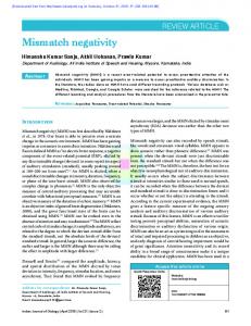
SEDF observations on black men is 533,198. Figure 1 provides a sense of what a zip code area is, relative to zip codes and to census blocks. We present three separate maps that contain information from the zip codes that begin with the number 600, which is essentially the city of Chicago. Chicago is of course just one particular example, but it is illustrative of many of the types of issues that arise in the study of spatial mismatch because it is a big city that has both high residential and high employment density in various parts of the city, and it is a raciallymixed city that is racially segregated. We constructed the first two maps in Figure 1 with GIS software using publicly-available data from the city of Chicago that are derived from the 2000 Decennial Census. The zip code boundaries are clearly delineated. In addition, in the first map each individual census block is color coded with the number of white residents living on the block and in the second map each census block is color coded with the number of black residents. In both cases, darker shades denote more residents. The third map in Figure 1 uses underlying data from County Business Patterns in 2000 and color codes the number of workers employed in each zip code. These maps do not directly display zip code areas – each defined as a zip code and all zip codes contiguous to it; zip code areas are too difficult to display as they often overlap. Nonetheless, it is clear from the first two maps in Figure 1 that zip code areas contain numerous census blocks, but do not cover large areas of land. The maps also reveal substantive information about spatial mismatch and the potential for racial mismatch. First, residential segregation is apparent, as areas of the city with high white residential density in general have low black residential density, and vice versa. Second, employment density in Chicago varies strongly across zip codes. A lot of workers are employed in downtown Chicago (and not so many Chicago residents live there). But there are many other areas of the city containing nontrivial employment as well. Moreover, although there appears to be a somewhat greater concentration of jobs near where whites live, there are also many jobs near where blacks live, suggesting that a simple disconnect between where blacks live and where jobs are located may not be the entire story. IV. Empirical Approach Spatial Mismatch 10

The analysis of spatial mismatch uses the sample of black men in the SEDF living in MSA’s. The first specification we estimate simply includes add an aggregate job density measure (JD) as well as a standard vector of controls, as in (1)

E = α + Xβ + δJD + ε .14 The spatial mismatch model implies that job density should be an important determinant of

employment, predicting that δ is positive. The variables in X include: age (linear and quadratic terms), marital status (a dummy variable for currently married), education (five dummy variables for high school degree, some college, Associate’s degree, Bachelor’s degree, and advanced degree), MSA fixed effects, and residence in a central city, non-central city, or suburb. Given the sample size, equation (1) is estimated as a linear probability model. Because the spatial mismatch model also predicts that the location of jobs is more relevant for less-skilled individuals, we augment the model to allow the effects of job density to vary with an individual’s education, as in (2)

E = α + Xβ + Σk δkJD⋅EDk + ε .

where EDk is a dummy variable for whether the individual has education level k.15 While equation (2) allows for different effects of overall job density depending on individuals’ skill levels, it may inaccurately capture the effects of job density on individuals in different skill groups because it uses an aggregate job density measure, rather than a measure of the density of jobs at skill levels closer to those of the worker. We therefore construct education-specific job density measures – in particular, for those with at most a high school degree, and for the narrower group of high school dropouts. When we construct these job density measures for lower education levels, the restriction applies 14

In most cases, because the data are clustered on zip code areas and the job density variables are defined at this level, we report standard errors that are robust to non-independence of observations within zip code areas, as well as heteroscedasticity. Estimated standard errors that are clustered at the MSA level are only slightly larger, and change none of the conclusions.

15

We experimented with varying levels of detail, but settled on using categories for less than high school, high school graduate, and any (some) college. Most of the important relationships appeared for the lowest levels of education, so there was nothing gained by further disaggregating those with different amounts of post-secondary education.

11

to both the numerator and the denominator; for example, the high school dropout job density measure is jobs held by high school dropouts divided by residents who are high school dropouts. Thus, equation (2) becomes (3)

E = αj + Xβj + Σk δkjJDj⋅EDk + εj , j=1,…, J,

where the job density measure now has a j subscript to indicate that it is defined for a particular education level, and the parameters have a j superscript (and the residual a j subscript) to indicate that we estimate the model separately for job densities defined for different education levels j. Under the spatial mismatch hypothesis, we expect to find the strongest evidence that job density affects employment of less-educated individuals using job density defined for low education groups. (We also estimate equation (1) for job densities defined for different education levels.) The estimates of the models in equations (1) through (3) provide increasingly detailed tests of whether the data are consistent with the spatial mismatch hypothesis. The overall results, and how they change with the specification, provide more compelling tests of the potential existence of spatial mismatch than has much of the previous literature. Racial Mismatch The specifications to this point do not distinguish job density by whether the jobs are held by blacks or by others. The racial mismatch hypothesis, however, implies that employment is more sensitive to job density for one’s own race – in contrast to the simple spatial mismatch hypothesis. To study this question, we first go back to the simplest specification (equation (1)), but we distinguish job density by race, as in (1’)

E = α + Xβ + δWJDW +δBJDB + ε . JDW is white jobs per black resident, and JDB is black jobs per black resident. We actually use

three alternative versions of these density measures: jobs held by non-blacks and jobs held by blacks, per black resident; jobs held by non-black men and jobs held by black men, per black male resident; and jobs held by white men and jobs held by black men, per black male resident. But as a short-hand the equation

12

simply refers to black and white job density.16 Because we define both densities relative to black residents, estimates of the two coefficients δW and δB allow a comparison of the effect on black employment probabilities of an additional black job per black resident to the effect of an additional white job per black resident. If job density of one’s own race is more important, then we should find that δB > δW (with the first expected to be positive), indicating that black job density does more to boost black employment. This would be evidence against pure spatial mismatch (which would instead predict no difference between δB and δW), and instead point to racial mismatch in the sense that black employment problems may reflect not so much the availability of jobs – at the right skill level in the specifications that distinguish by skill, described below – but rather jobs that are present but unavailable or less available to blacks.17 We also estimate equation (1’) for job densities defined for different education levels, and we estimate versions of equations (2) and (3) allowing for separate effects of job density by race. These specifications become (2’)

E = α + Xβ + Σk δkWJDW⋅EDk + Σk δkBJDB⋅EDk + ε

and (3’)

E = αj + Xβj + Σk δkj,WJDj,W⋅EDk + Σk δkj,BJDj,B⋅EDk + εj , j=1,…, J,

where JDj,B, for example, is jobs held by blacks with education level j per black resident with education level j. Again, comparisons of the estimated δ’s tell us whether the relationship between job density and employment – now based on skill – is race specific. We have already noted that a stronger association of black job density (perhaps by skill level) 16

The tables always clarify which group we are studying, but in the text we often simply refer to whites or to nonblacks.

17

A concrete example of what we are testing for is provided by the following example. Suppose that a new firm with 10 jobs is created in an area, and suppose that 9 of these jobs are filled by non-residents. We are told the racial mix of the 9 non-resident hires, and asked whether we can predict whether this new firm increases the probability that a random black in the area is employed. If racial mismatch matters, then this probability increases more if the 9 other hires are black than if the 9 other hires are white (i.e., the new firm increases black job density, rather than increasing white job density). The same argument holds if the 9 hires we are told about are not restricted to nonresident hires, as long as we leave the individual out of the calculation. In fact, we show later that our results are robust to excluding from the numerator all jobs held by residents, and instead defining job density as non-resident jobs per black resident.

13

than of white job density with black employment can arise from a number of sources, including discrimination, neighborhood, or peer effects. We know from the existing literature (most notably, perhaps, Manski’s 1993 and 2000 papers on the reflection problem) that it is very difficult to sort out these alternative explanations. Note, however, that our regressions are not plagued by the classic reflection problem that would arise if we were regressing individual employment on the mean local employment rate of black residents, because the numerator of the job density measures includes both residents and non-residents. We do not claim that we can distinguish between discrimination, neighborhood, and peer effects as potential explanations of the evidence of racial mismatch that we find. Rather, our contribution is to explore whether the relationship between an individual’s employment status and job density in one’s local labor market is driven by race-specific factors, which is inconsistent with the pure spatial mismatch hypothesis. V. Results Descriptive Statistics Panel A of Table 2 shows that 58% of black men, but only 30% of non-black men and 27% of white men live in central city areas, reflecting the rather profound residential segregation that is at the core of the spatial mismatch hypothesis. The panel also reveals the sharp educational differences between blacks and non-blacks or whites, with a much higher incidence of education less than high school (more than double the rate for whites), and a considerably higher incidence of post-secondary education for nonblacks (57%) and whites (62%) than for blacks (42%). Panel B reports on overall job density at the zip code area level, providing comparisons for blacks and whites.18 As reported in column (1), which covers all black and white men, job density is higher for black men, whether defined using men and women, only males, or only black and white males. The higher overall job density for blacks presumably reflects net commuting patterns into central city areas. Columns (2) and (3) report these statistics for lower education groups, and reveal no notable differences. The figures in Panel B contradict the basic tenet of the spatial mismatch hypothesis – quoted in

14

the Introduction – that “there are fewer jobs per worker in or near black areas than white areas.” However, this changes once we define job density by skill level, as shown in Panels C and D, which report job density figures broken down by education level – first based on those with at most a high school degree, and then high school dropouts. Job density for the lowest education category (less than high school) is lower for blacks (0.50 versus 0.66, in the first two rows of Panel D), and the same is true for job density based on a high school degree or less (0.64 for blacks versus 0.73 for whites in the corresponding rows); the same holds for densities defined using only males or only black and white males. In contrast, job density for those with some college (not shown in the table) is higher for blacks. The higher density at the highest education level, and lower density at lower education levels, highlight spatial mismatch in terms of skills, in that blacks, who are less educated, live in areas where high-skill job density is high relative to areas where whites live, while low-skill job density is relatively low. Table 3 reports job density figures by race, again overall and for two narrower education groups. These job density measures are used to capture “racial mismatch” rather than simply “spatial mismatch.” As we would expect given the small share of the black population, on average blacks are exposed to a much higher white or non-black job density than black job density. For example, in the first row of Panel A, the mean of overall non-black jobs per black resident is 6.11, versus a mean of black jobs per black resident of 0.61. The comparisons are similar for the lower education groups. The high value of non-black or white job density for black workers indicates that whites often hold many jobs in areas where blacks live; moreover, this is disproportionate to their share in the population of residents where blacks live.19 The much higher non-black job density does not necessarily imply, however, that there are many jobs available to blacks in the areas in which they live, because many of the jobs may require skill levels higher than those of local blacks. We would certainly expect this to some extent given the lower educational levels of blacks reported in Table 2. It is of interest, then, to compare the race-specific job 18

The figures for non-blacks are very similar to those for whites.

19

For example, we computed for blacks the mean of white male residents per black male resident, and the mean of white male jobs per black male job, based on zip code area of residence. The ratio of white male jobs to black male jobs exceeded the ratio of white male residents to black male residents by 25% (7.61 versus 6.11). At the lowest

15

density measures disaggregated by education level, which we do in Panels B and C of Table 3. The differences between non-black and black job density faced by blacks fall, indicating that the jobs held by non-blacks in areas where blacks tend to live employ more-educated workers. For example, in Panel C, for dropouts only, the average non-black job density is 4.30 (versus 6.11 across all education groups), while the average black job density is 0.46 (versus 0.61 across all education groups). Nonetheless, white job density is still considerably higher than black job density for these education-specific job density measures, so that less-educated blacks do live in areas where there are many jobs held by less-educated whites. This suggests that the problem may not be a lack of jobs at appropriate skill levels where blacks live, but a lack of jobs that are available to blacks. Spatial Mismatch Regressions Having discussed the descriptive statistics, we next turn to the regression results. We first report estimates of equations (1), (2), and (3), which include overall or education-specific job density measures, but without distinguishing the density measures by race. The top panel of Table 4 reports estimates of equation (1), using a single job density measure with no interactions with the individual’s education level. There are, though, two dimensions of variation across the nine columns of the table. First, we define density in three different ways: total jobs per resident; jobs held by males per male resident; and jobs held by black or white males (only) per black or white male resident. There is no obvious reason to prefer one of these density measures, but we want to explore the robustness of the results to the different measures. Second, we define this density based on all individuals as well as those with lower schooling levels. The spatial mismatch model predicts that job density defined for lower education levels should be a more important determinant of employment for low-skilled residents. The estimates in the top row of Table 4 indicate a statistically significant positive effect of job density on employment when the density is defined for either of the two lower education groups.20 For the overall density measure the effect is actually negative but it is much smaller and is insignificant in one of schooling level, the comparable numbers are 27% (4.40 versus 3.45). 20

Most of our key results are strongly statistically significant, so in the ensuing discussion we often avoid

16

the three cases, despite the large sample. Thus, the evidence points to a stronger effect of job density when it is calculated for jobs held by those with lower levels of education as a fraction of residents with the same levels of education. Moreover, the point estimates are always larger when job density is defined using those with the least education.21 To interpret the magnitudes, in column (6), for example, the estimate implies that a 0.1 (or 10 percentage point) increase in job density for high school dropouts, which is less than the difference between the 25th percentile and the median or the median and the 75th percentile, raises the probability of employment by 0.0042, or about 0.6 percent given the mean employment rate for black men, reported in Table 2, of 0.67. The specifications reported in the remaining rows of Table 4 distinguish the effects of job density on employment based on an individual’s own educational level. The spatial mismatch hypothesis predicts that job density should matter more for less-educated workers, and that this should be particularly true when job density is measured for individuals with less education. The estimates largely confirm these expectations. In all cases where job density is defined for the less-educated groups, we find a positive effect of job density on employment (e.g., the 0.099 estimate in column (3)), and this effect is always larger for the less-educated groups than those with some college. Moreover, in columns (2), (5), and (8), which define density based on those with at most a high school degree, the strongest effect of job density is for those with a high school degree (e.g., the estimate of 0.030 in column (5)), while in columns (3), (6), and (9), which define density based on high school dropouts, the strongest effect of job density is for that group. And finally, the strongest effects are found for high school dropouts when we define job density based on high school dropouts (e.g., the estimate of 0.076 in column (9)).22 Although these results are strongly consistent with spatial mismatch, it is possible that because of continually referring to the statistical significance of the results unless the conclusions differ. 21

Qualitatively similar results are reported in data for Sweden (Aslund et al., 2006).

22

It might appear curious that we find effects of education-specific density measures for individuals with other education levels – for example, the 0.070 estimate in column (9) for the effect of job density defined for high school dropouts on those with a high school degree. However, we do not include the density measures for workers with a high school degree in this regression, and the densities of jobs at different education levels are positively correlated. In addition, of course, there are not rigid lines between jobs at specific skill levels and the skill levels of workers; for example, a greater prevalence of jobs filled by those with less than a high school degree may nonetheless boost

17

endogenous sorting employment rates are higher in areas in which residents are more employable based on a set of unobserved person-specific characteristics, so that the relationship between job density and employment need not reflect spatial mismatch. While we obviously cannot control for all characteristics of workers, given that we are able to control for some key ones we are more inclined to interpret the variation in job densities as reflecting some kind of spatial influences. In addition, the evidence of stronger effects of the spatial distribution of jobs for those with less skill is an implication of the spatial mismatch model that does not derive nearly as naturally from the hypothesis of unobserved characteristics, given that there is no obvious reason that job density should serve as a stronger proxy for these unobservables for those with fewer skills relative to those with more skills.23 Racial Mismatch Regressions We now turn to our main evidence exploring whether there is a racial dimension to the effects of job density. To begin, columns (1), (4), and (7) of the top panel of Table 5 report estimates of equation (1’), where we simply use a measure of overall job density measure (not distinguished by education), although broken down by race.24 The estimates in these three columns indicate very clearly that only job density for blacks is substantively related to the employment of blacks. In each case, the estimated coefficient on the black job density measure is larger than that of the non-black job density measure by a factor of about 10. Next, just as we did in considering the pure spatial mismatch hypothesis, we measure job density based on lower educational levels – first for at most a high school degree (columns (2), (5), and (8)), and employment prospects of those with a high school degree even in these jobs. 23

The relationship between job density and employment could also arise from agglomeration economies that lead to higher worker productivity and hence higher wages where employment density is higher. However, Fu and Ross (2007) present evidence suggesting that this higher productivity is offset by commuting costs (which they argue reflects a locational equilibrium), leaving the net wage unaffected by employment density; in this case the job density results would not reflect a labor supply response to a higher wage stemming from agglomeration. And again, the agglomeration story does not explain the stronger effects of job density at lower skill levels.

24

Note that, relative to the job density measures in Table 4, these density measures utilize a different denominator defined only by black residents. We do this to isolate the role of job availability for black residents, rather than for all residents. As a result, the scale of the density measures in Table 5 is much larger than in Table 4 (see the summary statistics in Tables 2 and 3), which can affect the scale of the estimated regression coefficients in Table 5 relative to Table 4, irrespective of whether the effects of black job density and non-black job density differ.

18

then for high school dropouts (columns (3), (6), and (9)). We find that the estimated effects of non-black or white job density change by only a small amount, at most 0.0005. In contrast, the estimated effects of black job density are higher, rising by about 0.005 for the broader low-education group, and about 0.008 (roughly doubling) using the lowest-education group. The sharp differences in the estimated coefficients of the black versus the white or non-black job density measures indicate that black job density is a much more important determinant of black employment than is non-black job density. Moreover, the differences between the estimates in the first and second rows of Table 5 are strongly statistically significant. Based on these differences (and corresponding evidence below), we conclude that the racial mismatch hypothesis is a better characterization of how the spatial distribution of jobs affects black employment. In particular, from a policy perspective, we want to know which specification provides us with a better idea of how policy might be used to raise black employment. Our estimates make clear – and we show this with a simple simulation later – that the spatial mismatch model is clearly misleading, as it suggests that changing the spatial distribution of black residents could do a lot to increase black employment. In contrast, the racial mismatch model clarifies that simply shifting black residents to areas with high job density (even at the appropriate skill level) is unlikely to do much to increase black employment.25 The lower panel of Table 5 reports results for the specifications including interactions of the raceand education-specific job density measures with dummy variables for individuals’ education levels. The most important finding is that, regardless of the education level for which density is measured, the effect of black job density on black employment is much stronger than the effect of the corresponding non-black or white job density. In column (3), for example, the estimated effect of non-black job density defined for high school dropouts on employment of black high school dropouts is 0.0008, whereas the estimated 25

Note that some of the more standard statistical approaches do not apply when comparing the results in Tables 4 and 5. First, we cannot nest the models, because the denominators in the spatial and racial specifications are different; restricting the coefficients of black and white density in Table 5 to be the same in the racial mismatch specifications does not yield the spatial specification in Table 4. Moreover, the same policy argument above implies that the loss function that is minimized by maximizing R2 is not the right one. The goal is not simply to forecast variation in black employment, but rather to identify the types of policies more likely to be useful in increasing black employment.

19

effect on this same group of black job density defined for high school dropouts is 0.041. In general, the difference is much larger for less-educated workers, and in particular for the specifications defining job density for less-educated individuals the difference is sometimes a factor of 30, 40, or even more. We also find that the effect of black job density for less-educated blacks is stronger when this job density is defined based on less-educated workers and residents. For example, in the second row of the lower panel, the estimated effect of black job density on high school dropouts rises from 0.005 in column (1) to 0.041 in column (3). This always holds for the interactions with the dummy variables for the two lower education levels, although the same is not true for those with some college. Moreover, the estimated effect of black job density is particularly strong for less-educated blacks, when using the density measures defined for lower education levels. The causal interpretation of the 0.041 estimate in column (3) is that if black job density for high school dropouts increases by 0.1, the black high school dropout employment rate increases by 0.0041. Given an employment rate of 0.46 for black high school dropouts, this represents an increase of almost 1 percent. At the same time, the implied elasticity is well below 1, indicating that the benefit of higher job density does not accrue solely to residents. In contrast, we do not find the same sort of results with respect to the effects of non-black or white job density on black employment. Higher non-black or white job density has little relationship to black employment probabilities, and generally fails to exhibit the differences in effects associated with education that are predicted by the spatial mismatch hypothesis. Together, this evidence is consistent with the notion that the spatial distribution of job density matters for the employment of less-educated blacks, but it is only the spatial distribution of jobs held by blacks that matters – which we have termed racial mismatch. In Table 6 we examine the robustness of our results to other definitions of the local labor market, and therefore other measures of job density. In this and the ensuing robustness and other analyses we present, we report results for the specification in Table 5, column (6) (using men with less than a high school education to define job density).26 After repeating the baseline estimates in column (1), column (2) reports estimates using as our job density measure a distance-based gravity-like model of job access,

20

where we still use zip codes as the basic geographic construct but where we allow all jobs and residents across zip codes of an MSA to have an impact on measured job density. In particular, for each individual we first measure the distance between the centroids of his residential zip code and all other zip codes in the MSA. We then construct the numerator of the job density measure as the weighted sum across all zip codes in the MSA of the number of jobs in that zip code held by workers (with less than a high school education, and by race), using as weights 1/(1+distance)2. The denominator of the job density measure is the weighted sum of residents with the same characteristics in each zip code in the MSA, using the same weights. For any observation in our data, this weighting function obviously weights more strongly jobs and residents who live in the same zip code as the individual, with the weights decaying nonlinearly as we consider jobs and residents farther away from the zip code in which the individual resides. The estimates in column (2) of Table 6 are all higher than in column (1). For example, the effect of black job density on residents with less than a high school education in column (2) is 0.123, three times larger than in the baseline specification. This is not surprising, given that the gravity-based job density measures incorporate jobs in the entire MSA, rather than just in the zip code area. But the important qualitative results still hold. In particular, black job density matters much more than non-black job density for employment, and matters most for less-skilled residents. In column (3) we use a weighting function of 1/(1+distance), which decays at a slower rate with distance. The estimates on black density, in particular, are even higher, but again the results show strong differences in the impact of job density by race, and much stronger impacts of black job density on less educated blacks relative to those with some college education. In column (4) we take the opposite approach to weighting, using an extreme job density measure which defines job density to consist of jobs per resident only for the exact zip code in which the individual resides. For the most part, the results are very similar to those in the baseline results reported in column (1). All in all, the results in Table 6 find robust evidence in support of racial mismatch. We next consider a number of additional analyses that assess potential sources of bias in our 26

Results were similar for other specifications based on measures of job density for those with low education.

21

estimates or help to interpret the estimates. First, if blacks and whites live in different types of zip codes, and this causes the mismeasurement of the local labor market to differ by race, then any comparisons of the effects of job density across races might be misleading. Perhaps of most concern is the fact that zip codes are larger in suburban areas. For example, if in suburban areas the local labor market is more likely to be just the zip code of residence, rather than contiguous zip codes as well, then white job density in the suburbs is overstated relative to white job density in central cities when we use contiguous zip codes everywhere. Thus, depending on whether the identification of the black and white job density effects comes more from observations concentrated in the city versus the suburbs, the relative magnitudes of these estimated effects may be biased. This problem should be addressed by the gravity-type estimates reported in Table 6. As another approach, however, we re-estimated our racial mismatch regressions excluding suburban residents. The evidence for the same comparison specification is reported in column (2) of Table 7, and is qualitatively similar to that from the baseline specification, with at most a slight diminution of the estimated differences between the effects of black and non-black job density. Second, we consider a specification that may help to separate the influence of unobservables such as neighborhood or network effects that are common to residents of a local labor market from the influence of job availability per se, and hence go some way toward assessing the importance of the possible mechanisms that could drive our results. In particular, the black job density measure JDB in equation (2’) can be rewritten as (JDBR +JDBNR) where JDBR is the number of jobs held by black residents of the zip code area per black resident, and JDBNR is the number of jobs per black resident held by black non-residents. We estimate a specification in which we incorporate both of these job density measures (again, by race and skill) separately into the employment equation and examine to what extent an individual’s employment is differentially associated with the resident and non-resident job density measures.27 To the extent that the zip code area defines an area in which residents are more likely to be similar in unobservable ways than others who work there – for example by experiencing common neighborhood effects – we expect the resident job density measure (JDBR) to pick up the effects of these

22

factors on employment and hence to be the source of the findings reported thus far. In contrast, we expect any effects of the non-resident density measure (JDBNR) to capture the impact of job availability, which may reflect labor market discrimination. Columns (3a) and (3b) of Table 7 report the estimates from regressions including both resident and non-resident job density measures.28 In general, the disaggregated job density results from this regression show that the estimates based on the aggregate race-specific job density measure that we used in the preceding results are very similar to those identified for non-resident jobs in the zip code area, while the estimates for resident job density are much larger. In the top panel, the estimated effects of both non-black resident and non-black non-resident jobs are small (0.001 and 0.0001) and are of a scale that is similar to that of the baseline specification in column (1) (0.0003). In contrast, the estimate of the black resident job density coefficient is very large (0.154), whereas the estimate of the non-resident job density measure is 0.014, close to the estimate of 0.018 for the aggregated density measure. The similarity of the latter two estimates implies that the aggregate estimates mainly reflect the effects of non-resident job density. When we estimate separate effects by interacting the resident and non-resident job densities with an individual’s education, as reported in the bottom panel of the table, the impacts on those with some college are again very small for both density measures. For those with lower levels of education, the estimated impact of the black resident density measures again are very large, whereas the estimated impact of the non-resident black job densities, while somewhat smaller than in the baseline results, is still of the same order of magnitude and is always stronger than the non-black density measure. The fact that the estimated effect in column (3a) of low-skilled resident black job density on employment of low-skilled blacks is so large suggests that it probably reflects unobservables shared by local residents, including neighborhood or network effects. But the fact that, even conditional on resident job density, the job density of low-skilled black male non-residents is strongly related to the employment 27

In each case, the denominator remains the same as in the baseline.

28

Conditional on the other covariates included in the model, the correlation between resident and non-resident black job density is only 0.05. The corresponding correlation for non-blacks is 0.61. (The unconditional correlations are virtually the same.)

23

of low-skilled resident black males (column (3b)) suggests to us that there likely is a direct and substantive role for the local availability of jobs for lower-skilled blacks to affect the employment of lowskilled black male residents, possibly stemming from labor market discrimination.29 A third issue we consider is that there may be measurement error in the job density measures resulting simply from sampling error – most likely because of zip code areas with very few black men, given their small share of the population. Unlike the textbook measurement error case, the implications for bias in the estimated coefficients are unclear, because we always have more than one density measure included in the equation, and we often also have interactions between these density variables and education. To assess the potential influence of measurement error on the estimates, we re-estimated our models dropping from the sample zip code areas for which density measures were based on fewer than 10 black men. We report the results in column (4) of Table 7. In the top panel, using job density measures without the education interactions, the estimated effect of non-black job density rises, and that of black job density falls relative to the baseline specification, although the black job density still remains much larger. For the estimates in the bottom panel that include the education interactions, the estimated effects of job density based on high school dropouts are actually larger for high school dropouts and for those with at most a high school degree, but not for those with some college. For the two low-education groups, for which the spatial distribution of jobs should be more important, the differences between the estimated effects of black and non-black job density increase. Thus, we regard the evidence for the two loweducation groups as largely unchanged.30 A different measurement issue is whether the flow of new jobs better captures job availability than the stock of jobs as embodied in job density measures like the ones we use. Raphael (1998), in work that addresses pure spatial mismatch, instead uses job creation rates to measure job availability, based on 29

It is also possible, in principle, that even conditional on education and the other controls in our model, there is some sense in which black jobs are more suited to black workers, and similarly for white jobs and white workers. This is clearly always an alternative explanation to discrimination in hiring. However, we view this alternative explanation as less plausible because the qualitative results are insensitive to the inclusion or exclusion of the demographic controls we do observe, making it less likely that unobservable job characteristics drive the results.

30

We also verified that the estimates and conclusions were robust to omitting the weighting to correct for the non-

24

employment change between the 1980 and 1990 Censuses. However, even if job changes matter more than job levels for characterizing the spatial distribution of employment opportunities, unless the relationship between job flows and stocks differs for jobs held by blacks and jobs held by whites, the fact that we use a stock measure of job availability rather than a flow measure cannot explain the difference in the impact of job density by race in our estimates. This argument echoes one we make a few times in this section; although one can think of reasons why the estimated coefficients on job density measures in our regressions corresponding to pure spatial mismatch may be biased estimates of the effects of the local availability of jobs, it is far less clear why there is any bias in the estimated differences between the coefficients of the white and black job density measures. Fourth, as noted earlier, the importance of spatial influences on employment outcomes is predicated on constraints on residential mobility. Most of the empirical work in the spatial mismatch literature has taken residential location as exogenous, as do we. In tests of pure spatial mismatch, this is a potentially serious concern, as those with stronger tastes for work or higher market productivity may choose to locate in areas with more jobs, hence generating a positive association between job density and employment probabilities.31 However, this factor alone does not explain why there is a much larger coefficient estimate on black job density than on white job density, as the blacks with stronger tastes for work should relocate to areas with higher job density irrespective of the racial composition of those jobs. Rather, our findings could be generated by endogenous residential mobility only if blacks with stronger tastes for work (or higher productivity) tend to move to areas where there are relatively more jobs employing blacks. But the results would still imply that these blacks are not, to the same extent, moving representativeness of the sample with valid place of work. 31

Aslund et al. (2006) study this question for refugees in Sweden by exploiting a policy that dispersed refugees to different regions of the country in a way that was arguably random conditional on the observables available to them. They find positive effects of job density regardless, except for highly-educated groups, but they find considerably stronger estimates of job density when they study this refugee sample (for employment outcomes in 1999 regressed on job density measures where they were assigned in 1990-91), compared with a cross-section of the population or even simply the 1999 cross-section for refugees, who may have moved subsequent to original assignment in 199091. If endogenous sorting is important, this result is surprising, because the endogenous sorting would be expected to lead to upward bias in the estimated relationship between job density and employment.

25

to areas where there are relatively more jobs employing non-blacks.32 In that sense, even if blacks with stronger tastes for work were moving to areas with higher black employment rates, the results would still demonstrate the importance of the race-specific spatial distribution of jobs, rather than the spatial distribution of jobs per se. Nonetheless, we can also shed some light on whether our results are driven by mobility. In columns (5) and (6) of Table 7, we break the sample into those who did not change residence in the last 5 years, and those who moved in that period. We find similar results for both subsamples. We cannot necessarily interpret the results for those who did not move in the last 5 years as representing effects for individuals who are completely immobile. But this subsample is clearly less mobile, and given that lowskilled workers are likely to be in relatively high-turnover jobs, it seems reasonable to view residential location for this sample as predetermined with respect to employment. In general, therefore, our evidence on the effects of race-specific job density is very robust, and does not appear to suffer from biases that might generate spurious evidence of racial mismatch.33 In the final regression estimates we present, we switch to studying how white and non-white job density affect the employment of white men. These estimates are reported in Table 8, and reveal qualitatively similar results to what we found for blacks, with white male job density strongly positively associated with higher employment of whites, and more so for less-educated white workers and for density measures based on less-educated workers. Indeed the estimated coefficients on the non-white job density variables are negative, although very small and in some cases insignificant.34 Thus, for whites we get the same kind of evidence of racial mismatch as we do for blacks, suggesting that the racial distribution of jobs, and not only the spatial distribution, matters for both whites and blacks. One might, 32

The same argument would apply if the racial mismatch results are driven by the reverse story, where employers that employ blacks are attracted to areas where blacks are more likely to be employed. In this case, too, absent the racial dimension underlying employers’ location decisions, the evidence of racial mismatch would not arise.

33

We also did many of these robustness checks for the pure spatial mismatch tests in Table 4, and found, similarly, that the results in that table were very robust.

34

It is possible that the negative coefficient estimates can be explained by low unobservables related to employment for whites living in areas of high black job density (conditional on white job density).

26

however, be more inclined to view the results for whites as driven by networks than by employer discrimination, although co-worker discrimination on the part of both blacks and whites could also generate these results. Quantifying the Importance of Spatial Mismatch We first presented evidence from a new approach to testing for spatial mismatch, based on job density, and found evidence consistent with the predictions of the model, suggesting that black employment probabilities are lower where job density in their residential area is lower, and that this relationship is stronger at lower educational levels. We then showed, however, that it is the race-specific job densities that matter; job density for blacks is much more strongly related to black employment probabilities than is white job density. What does this evidence imply? At the risk of employing a double negative, it does not imply that space does not matter. Blacks living in areas of higher black job density do have higher employment probabilities. But the impact of space has a strong racial dimension, as higher job density for non-blacks has very weak effects on black employment probabilities. Thus, the evidence does not reject spatial mismatch per se, but it rejects what we have termed “pure spatial mismatch” – that is, that the spatial distribution of jobs, per se, is an important determinant of black employment, and in particular that a significant determinant of the lower employment of blacks living in central city areas is the simple lack of nearby jobs. One way to try to make this conclusion more concrete is to ask what the estimates imply for the importance of pure spatial mismatch for black employment. In order to gauge the impact of space, per se, on black employment, we use the coefficients that we estimate in our employment model, but calculate the employment probability that would be implied if a black man lived where the representative non-black or white lived. We do this calculation for black and white males, restricting attention to high school dropouts, for whom spatial mismatch (whether race-specific or not) is most important. Table 9 lays out the steps of this calculation.35 35

This simulation ignores any general equilibrium effects of many people moving, and is therefore best thought of as calculating the change in predicted employment if a small number of black males moved to areas in which they faced the job densities of the representative white male in their MSA. If we do this calculation for the broader low-skill group with at most a high school education or for black and non-black males, we reach a very similar conclusion to that described below.

27

In Panel A, we report the mean employment rates by race for male high school dropouts. For this group, the mean employment rate for blacks is 0.459, compared with 0.690 for whites, a gap of 0.231. Next we report estimates from the simplest model with race-specific job densities. The model is equivalent to that in the last column of the top panel of Table 5, but using the sample of black male high school dropouts only. As reported in Panel B, the estimates reflect the same finding as before; the estimated effect of black job density is more than 10 times that of white job density. Panel C reports the means of the job density measures for blacks. There are considerably more white male jobs per black resident than black male jobs per black resident, averaged across blacks. In Panel D, we instead compute the means of the same job density measures that blacks would face if they lived where the representative white in their MSA lived.36 Comparing Panels C and D, it is clear that whites on average live in areas where there are more jobs per black resident, whether held by whites or by blacks, although the difference is far greater for jobs held by whites. Finally, we predict employment probabilities using the estimated employment model from which the coefficients in Panel B come, but substituting the job density measures in Panel D for those in Panel C (the latter are the means for blacks, which along with the means of the other variables and their coefficients yield the mean employment rate for blacks). Because both job density estimates in Panel D are higher, this obviously results in a higher predicted employment rate for blacks. However, because the effect on black employment of white job density – which is what would increase most sharply if blacks lived where whites lived – is so small (0.002), the simulated change in residential location has very little effect on the predicted probability of employment for blacks. Overall, the new predicted black probability is only higher than the actual mean by 0.025, which is a small share (10.8 percent) of the race difference in employment rates for these groups.37 We interpret these results as indicating that space, per se, has 36

We calculate this by computing the average job densities (on a per black resident basis) for white male high school dropouts. We then take the mean across whites in the MSA, assign these to each black based on their MSA of residence, and then average across blacks.

37

The 0.025 result comes from the combination of two effects that occur when we reallocate blacks to where whites live: the increase in white job density of 5.883 (7.868 – 1.985) multiplied by 0.002 yields an effect of 0.0118 (or 1.18 percentage points); and the increase in black job density of 0.454 (0.886 − 0.432) yields an effect of 0.0127. If

28

relatively little to do with lower black employment among those with less education, although the effect is not zero. VI. Conclusions According to the spatial mismatch hypothesis, the location of jobs coupled with residential segregation and mobility barriers and costs combine to reduce black employment rates, especially among those with lower skills. We contrast the spatial mismatch hypothesis with what we term the racial mismatch hypothesis – or spatial-racial mismatch, to emphasize that space also plays a role, but that race is central. The racial mismatch hypothesis suggests that the problem is not a lack of jobs, per se, where blacks live, but a lack of jobs into which blacks are hired, whether because of discrimination, labor market networks, or neighborhood effects in which race matters. Under the racial mismatch hypothesis, it is the local availability of jobs for (or held by) members of one’s own race that matters for employment. We begin by reporting evidence on the spatial mismatch hypothesis. We take advantage of access to all Census Long-Form respondents to study the relationship between employment and location-specific measures of the distribution of jobs, conditional on skill. When we construct direct measures of the presence of jobs in detailed geographic areas, we find that these job density measures are related to black employment in ways that would be predicted by spatial mismatch. In particular, black employment is higher in areas with more jobs per resident. Moreover, this is true primarily for low-skilled jobs and residents, as the density of jobs for those with less than a high school degree has a stronger effect on black employment, and the strongest effect for the least-skilled blacks. We then move beyond considering pure spatial mismatch to look at racial mismatch, estimating the effects of job density measures that are disaggregated by race. The findings are quite striking. It is instead of reallocating blacks, we simply had a way to make the effect of white job density on black employment as large as the effect of black job density, then black employment would be much higher (by 1.985 multiplied by 0.028 instead of 0.002, or 5.6 percentage points). And of course if we could do both – eliminating the spatial difference by race, as well as the differential effects of white versus black job density – the effect would be even larger, 0.028 ·(5.883+0.454) or 17.7 percentage points. However, note that it is not clear that, in the absence of the factors that generate different effects of black and white job density on black employment, the coefficient on white job density would be the one that would prevail. Instead, some number between 0.002 and 0.028 might be more likely. This issue has parallels to the question, in studies of wage discrimination, of what the wage structure would look like if there were no discrimination (Neumark, 1988). Here, though, it is likely even more complicated because

29

primarily black job density that influences black employment, whereas white (or non-black) job density has little if any influence on the employment of blacks. Moreover, we find similar patterns with respect to differences in effects associated with schooling; black job density at lower education levels has a stronger effect on employment of blacks, and in particular for those blacks with less education. This evidence does not repudiate the importance of the spatial distribution of jobs. What it suggests, however, is that race plays a key role, and that the availability of jobs locally is not enough to markedly impact black employment rates. Pure spatial mismatch is not an important component of lower black employment rates. Instead the spatial distribution of jobs available to blacks – or racial mismatch – appears to be much more important. This evidence has potentially significant implications for policies designed to counter what has been interpreted as pure spatial mismatch. Specifically, concerns over spatial mismatch have helped motivate policy interventions such as “Moving to Opportunity” (Katz et al., 2001), “Wheels to Work” and other programs to increase access of low-income workers to cars (Goldberg, 2001), and enterprise zones (Peters and Fisher, 2002). Interestingly, many evaluations of these programs suggest that they are relatively ineffective at increasing black employment. This is entirely consistent with the results we find here, where simply living near jobs, even at one’s skill level, does little to boost black employment unless those jobs are available (or tend to be held by) blacks. Indeed, a simple simulation shows that moving blacks so that they faced the race-specific job densities of the representative white in their MSA (with the same skill level) would do relatively little to increase black employment, because the main effect of such a move would be to expose them to higher white (or non-black) job density, which our estimates indicate does little to increase black employment. Our results demonstrate that formal descriptions and empirical tests of the process by which the spatial distribution of jobs matters for black employment must take seriously the modeling of the mechanism(s) by which race matters. We previously mentioned some obvious mechanisms for which there is already some empirical support – discrimination, labor market networks, and neighborhood discrimination may not be the only source of racial mismatch.

30

effects – but there may be others as well. It remains an important task for future research to try to disentangle the separate impacts of these mechanisms in explaining why more jobs held by whites or nonblacks in a local area has little effect on black employment rates. A better understanding of these factors can facilitate the choices among and the design of policies to increase black employment, especially among the less skilled.

31

References Aslund, Olof, John Osth, and Yves Zenou. 2006. “How Important is Access to Jobs? Old Question – Improved Answer.” Unpublished paper, Institute for Labour Market Policy Evaluation, Uppsala, Sweden. Bayer, Patrick, Stephen Ross, and Giorgio Topa. 2005. “Place of Work and Place of Residence: Informal Hiring Networks and Labor Market Outcomes.” NBER Working Paper No. 11019. Bertrand, Marianne, and Sendhil Mullainathan. 2004. “Are Emily and Greg More Employable Than Lakisha and Jamal? A Field Experiment on Labor Market Discrimination.” American Economic Review, Vol. 94, No. 4, pp. 991-1013. Brueckner, Jan K., and Stuart S. Rosenthal. 2005. “Gentrification and Neighborhood Housing Cycles: Will America’s Future Downtowns be Rich?” CESifo Working Paper No. 1579. Case, Anne C., and Lawrence F. Katz. 1991. “The Company You Keep: The Effects of Family and Neighborhood on Disadvantaged Youth.” NBER Working Paper No. 3705. Combes, Pierre-Philippe, Gilles Duranton, and Laurent Gobillon. “Spatial Wage Disparities: Sorting Matters!” Forthcoming in Journal of Urban Economics. Cutler, David M., Edward L. Glaeser, and Jacob L. Vigdor. 1997. “The Rise and Decline of the American Ghetto.” NBER Working Paper No. 5881. Cutler, David M., and Edward L. Glaeser. 1997. “Are Ghettos Good or Bad?” Quarterly Journal of Economics, Vol. 112, No. 3, August, pp. 827-72. Ellis, Mark, Richard Wright, and Virginia Parks. “Geography and the Immigrant Division of Labor.” Forthcoming in Economic Geography. Ellwood, David. 1986. “The Spatial Mismatch Hypothesis: Are There Jobs Missing in the Ghetto?” In The Black Youth Employment Crisis, eds. Freeman and Holzer (Chicago: University of Chicago Press), pp. 147-85. Evans, William N., Wallace E. Oates, and Robert M. Schwab. 1992. “Measuring Peer Group Effects: A Study of Teenage Behavior.” Journal of Political Economy, Vol. 100, No. 5, October, pp. 966-91. Fu, Shihe, and Stephen L. Ross. 2007. “Wage Premia in Employment Clusters: Agglomeration Economies or Worker Heterogeneity?” University of Connecticut, Department of Economics Working Paper No. 2007-26. Glaeser, Edward L., Matthew E. Kahn, and Jordan Rappaport. 2006. “Why Do the Poor Live in Cities? The Role of Public Transportation.” Working Paper No. 2007-12, UCLA Ziman Center for Real Estate. Glaeser, Edward L. and David Mare. 2001. “Cities and Skills.” Journal of Labor Economics, Vol. 19, No. 2, April, pp. 316-42. Goldberg, Heidi. 2001. “State and County Supported Car Ownership Programs Can Help Low-Income Families Secure and Keep Jobs.” Center on Budget and Policy Priorities, November 28, available at http://www.cbpp.org/11-8-01wel.htm (as of October 28, 2005). Granovetter, Mark S. 1974. Getting a Job: A Study of Contacts and Careers (Cambridge, MA: Harvard

University Press). Harrison, Bennett. 1972. “The Intrametropolitan Distribution of Minority Economic Welfare.” Journal of Regional Science, Vol. 12, No. 1, April, pp. 23-43. Holzer, Harry J. 1991. “The Spatial Mismatch Hypothesis: What Has the Evidence Shown?” Urban Studies, Vol. 28, No. 1, February, pp. 105-22. Hughes, Mark A., and Janice Madden. 1991. “Residential Segregation and the Economic Status of Black Workers: New Evidence for an Old Debate.” Journal of Urban Economics, Vol. 29, No. 1, January, pp. 28-49. Ihlanfeldt, Keith R. 1992. Job Accessibility and the Employment and School Enrollment of Teenagers (Kalamazoo, MI: W. E. Upjohn Institute for Employment Research). Ihlanfeldt, Keith R., and David Sjoquist. 1990. “Job Accessibility and Racial Differences in Youth Employment Rates.” American Economic Review, Vol. 80, No. 1, March, pp. 267-76. Ihlanfeldt, Keith R., and David Sjoquist. 1998. “The Spatial Mismatch Hypothesis: A Review of Recent Studies and Their Implications for Welfare Reform.” Housing Policy Debate, Vol. 8, No. 4, pp. 849-92. Kain, John. 1968. “Housing Segregation, Negro Employment, and Metropolitan Decentralization.” Quarterly Journal of Economics, Vol. 82, No. 2, May, pp. 175-97. Katz, Lawrence F., Jeffrey R. Kling, and Jeffrey B. Liebman. 2001. “Moving to Opportunity in Boston: Early Results of a Randomized Mobility Experiment.” Quarterly Journal of Economics, Vol. 116, No. 2, May, pp. 607-54. Manski, Charles. 1993. “Identification of Endogenous Social Effects: The Reflection Problem.” Review of Economic Studies, Vol. 60, No. 3, July, pp. 531-42. Manski, Charles. 2000. “Economic Analysis of Social Interactions.” Journal of Economic Perspectives, Vol. 14, No. 3, Summer, pp. 115-36. Neumark, David. 1988. “Employers’ Discriminatory Behavior and the Estimation of Wage Discrimination.” Journal of Human Resources, Vol. 23, No. 3, Summer, pp. 279-95. Peters, Alan H., and Peter S. Fisher. 2002. State Enterprise Zone Programs: Have They Worked? (Kalamazoo, MI: W. E. Upjohn Institute for Employment Research). Price, Richard, and Edwin Mills. 1985. “Race and Residence in Earnings Determination.” Journal of Urban Economics, Vol. 17, No. 1, January, pp. 1-18. Raphael, Steven. 1998. “The Spatial Mismatch Hypothesis of Black Youth Joblessness: Evidence from the San Francisco Bay Area.” Journal of Urban Economics, Vol. 43, No. 1, January, pp. 79-111. Rosenthal, Stuart S., and William C. Strange. 2008. “The Attenuation of Human Capital Spillovers.” Unpublished paper, Syracuse University. Ross, Stephen L. 1998. “Racial Differences in Residential and Job Mobility: Evidence Concerning the Spatial Mismatch Hypothesis.” Journal of Urban Economics, Vol. 43, No. 1, pp. 112-35.

Turner, Margery A., Michael Fix, and Raymond J. Struyk. 1991. Opportunities Denied, Opportunities Diminished: Racial Discrimination in Hiring (Washington, DC: Urban Institute Press). Vrooman, John, and Stuart Greenfield. 1980. “Are Blacks Making It in the Suburbs? Some New Evidence on Intrametropolitan Spatial Segmentation.” Journal of Urban Economics, Vol. 7, No. 2, March, pp. 15567. Weinberg, Bruce. 2000. “Black Residential Centralization and the Spatial Mismatch Hypothesis.” Journal of Urban Economics, Vol. 48, No. 1, pp. 110-34. Weinberg, Bruce. 2004. “Testing the Spatial Mismatch Hypothesis Using Inter-City Variations in Industrial Composition.” Regional Science and Urban Economics, Vol. 34, No. 5, September, pp. 505-32. Wilson, William Julius. 1987. The Truly Disadvantaged (Chicago: University of Chicago Press). Zax, Jeffrey, and John F. Kain. 1998. “Moving to the Suburbs: Do Relocating Companies Leave Their Black Employees Behind?” Journal of Labor Economics, Vol. 14, No. 3, July, pp. 472-504.

Figure 1: Chicago Population and Employment Statistics

Table 1: SEDF Sample

Full SEDF (not institutionalized)

(1) Total 42,583,178

(2) Black males ...

Restrict to men

20,713,501

2,163,218

Not in CMSA/MSA

...

377,562

Not in age range 16-64

...

890,056

In military

...

13,556

Enrolled in school

...

905,359

Work limiting disability

...

259,636

Exclusion criteria (total cases):

SEDF observations retained

700,303

Live in water zip

2,888

Work in water zip

2,816

Observations with unmatched or allocated place of work location

...

Total observations remaining for calculation of densities Observations dropped because of missing densities, insufficient population size

158,989 535,677

...

2,479

Final sample 533,198 SEDF: Sample Edited Detail File of all Long-Form Census respondents. The exclusion criteria are not mutually exclusive, so many observations show up in multiple rows.

Table 2: Comparisons of Individual Characteristics and Overall Job Density Measures by Race (1) (2) (3) A. Individual characteristics (means): Non-black White Black men men men Employment .67 .84 .86 Individual characteristics: Central city .58 .30 .27 LTHS .24 .16 .10 HSD .34 .27 .28 SCOL .42 .57 .62 B. Job density measures (All) Mean (SD) LTHS+HSD LTHS Jobs/residents Blacks .77 (.51) .77 (.51) .79 (.55) Whites .73 (.40) .67 (.33) .68 (.34) Male jobs/male resident Blacks .87 (.57) .88 (.56) .90 (.60) Whites .80 (.45) .74 (.37) .75 (.39) Black and white male jobs/black and white male residents Blacks .91 (.63) .92 (.63) .94 (.67) Whites .81 (.48) .76 (.41) .77 (.44) C. Job density measures (LTHS + HSD) Mean (SD) LTHS+HSD LTHS Jobs/residents Blacks .64 (.41) .62 (.36) .62 (.37) Whites .73 (.51) .64 (.34) .63 (.35) Male jobs/male resident Blacks .75 (.47) .73 (.41) .72 (.42) Whites .83 (.58) .73 (.39) .72 (.40) Black and white male jobs/black and white male residents Blacks .78 (.52) .76 (.47) .76 (.48) Whites .84 (.60) .74 (.41) .74 (.43) D. Job density measures (LTHS) Mean (SD) LTHS+HSD LTHS Jobs/residents Blacks .50 (.34) .47 (.28) .46 (.28) Whites .66 (.50) .57 (.32) .55 (.33) Male jobs/male resident Blacks .61 (.40) .58 (.33) .57 (.33) Whites .78 (.59) .67 (.38) .65 (.40) Black and white male jobs/black and white male residents Blacks .62 (.40) .59 (.35) .58 (.35) Whites .75 (.52) .66 (.36) .64 (.36) There are 533,198 observations on black men, and 4,030,425 on white men, using the sample construction rules in Table 1. Standard deviations (SD) of continuous variables are reported in parentheses in Panels B through D. All estimates are weighted to account for differences in the probability of having valid place of work data. “LTHS” refers to those without a high school diploma, “HSD” represents high school graduates, and “SCOL” refers to those with at least some college education, including college graduates.

Table 3: Race-Specific Job Density Measures for Black Men (1) (2) Mean (SD) LTHS+HSD A. Overall

(3) LTHS

Non-black jobs/black residents

6.11 (13.75)

5.25 (12.19)

4.83 (11.82)

Non-black male jobs/black male residents

6.92 (14.16)

6.03 (12.38)

5.59 (11.92)

White male jobs/black male residents

5.75 (12.39)

5.07 (10.89)

4.67 (10.41)

Black jobs/black residents

.61 (.64)

.57 (.53)

.57 (.53)

Black male jobs/black male residents

.62 (.62)

.59 (.52)

.59 (.52)

Non-black jobs/black residents

4.96 (14.03)

4.06 (12.02)

3.61 (10.64)

Non-black male jobs/black male residents

5.59 (14.32)

4.65 (12.33)

4.19 (11.45)

White male jobs/black male residents

4.05 (11.58)

3.48 (10.12)

3.09 (9.12)

Black jobs/black residents

.55 (.80)

.50 (.60)

.48 (.58)

Black male jobs/black male residents

.58 (.78)

.53 (.60)

.52 (.58)

Non-black jobs/black residents

4.30 (12.72)

3.34 (10.55)

2.91 (10.02)

Non-black male jobs/black male residents

5.54 (16.03)

4.34 (13.11)

3.84 (12.69)

White male jobs/black male residents

2.73 (8.03)

2.29 (6.95)

1.98 (6.33)

.46 (.75)

.41 (.57)

.39 (.53)

B. LTHS + HSD

C. LTHS

Black jobs/black residents

Black male jobs/black male residents .51 (.75) .45 (.59) .43 (.55) There are 533,198 observations. Standard deviations (SD) of continuous variables are reported in parentheses. All estimates are weighted to account for differences in the probability of having valid place of work data.

Table 4: Employment Regressions for Black Men, Alternative Aggregate Density Measures, With and Without Own Education Interactions, Contiguous Zip Codes, MSA Fixed Effects (1) (2) (3) (4) (5) (6) (7) (8) (9) Job density Black or white male jobs/ measure: Jobs/resident Male jobs/male resident black or white male resident Job density defined for: All LTHS+HSD LTHS All LTHS+HSD LTHS All LTHS+HSD LTHS Job density -.005 .028 .052 -.006 .022 .042 -.008 .018 .045 (.003) (.003) (.006) (.002) (.002) (.004) (.002) (.002) (.003) R2

.139

.139

.140

.139

.139

.140

.139

.139

.140

Jobs/resident × own education LTHS

-.018 (.004)

.033 (.006)

.099 (.012)

-.019 (.004)

.024 (.005)

.075 (.008)

-.019 (.003)

.018 (.005)

.076 (.007)

Jobs/resident × own education HSD

-.010 (.004)

.040 (.005)

.093 (.010)

-.012 (.003)

.030 (.005)

.072 (.007)

-.013 (.003)

.023 (.004)

.070 (.006)

Jobs/resident × own education SCOL

.007 (.002)

.021 (.002)

.027 (.004)

.005 (.002)

.017 (.002)

.022 (.003)

.003 (.002)

.015 (.002)

.025 (.003)

.139 .140 .141 .139 .139 .141 .139 .139 .141 R2 There are 533,198 observations on blacks. Regression estimates are from linear probability models, with standard errors in parentheses. All specifications include controls for age (linear and quadratic terms), marital status (a dummy variable for currently married), highest education (six categories including less than high school, high school degree, some college, Associate’s degree, Bachelor’s degree, and advanced degree), residence in the central city, noncentral city, and suburban residence, and MSA fixed effects. All estimates are weighted to account for differences in the probability of having valid place of work data. All standard errors are robust to non-independence of observations within zip code areas heteroscedasticity. See also notes to Table 2.

Table 5: Employment Regressions for Black Men, Alternative Race-Specific Density Measures, With and Without Own Education Interactions, Contiguous Zip Codes, MSA Fixed Effects (1) (2) (3) (4) (5) (6) (7) (8) (9) Job density Non-black jobs or black jobs/ Male non-black jobs or male black jobs/ Male white jobs or male black jobs/ measure: black resident black male resident black male resident Job density defined for: All LTHS+HSD LTHS All LTHS+HSD LTHS All LTHS+HSD LTHS Non-black or white .001 .001 .0005 .0008 .0005 .0003 .0009 .0006 .0005 job density (.0001) (.0001) (.0001) (.0001) (.0001) (.0001) (.0001) (.0001) (.0002) Black job density

.008 (.002)

.013 (.002)

.016 (.003)

.009 (.002)

.013 (.002)

.018 (.002)

.010 (.002)

.014 (.002)

.018 (.002)

.140

.140

.140

.140

.140

.140

.140

.140

.140

Non-black jobs/ black resident × own educ. LTHS

.002 (.0002)

.001 (.0002)

.0008 (.0002)

.002 (.0003)

.001 (.0002)

.0004 (.0001)

.002 (.0003)

.001 (.0002)

.001 (.0003)

Black jobs/ black resident × own educ. LTHS

.005 (.004)

.026 (.006)

.041 (.007)

.005 (.005)

.027 (.005)

.041 (.005)

.006 (.005)

.027 (.005)

.038 (.005)

Non-black jobs/ black resident × own educ. HSD

.002 (.0001)

.001 (.0002)

.0008 (.0002)

.001 (.0001)

.0009 (.0001)

.0005 (.0001)

.002 (.0002)

.001 (.0002)

.001 (.0002)

Black jobs/ black resident × own educ. HSD

.009 (.004)

.024 (.004)

.028 (.006)

.009 (.004)

.024 (.004)

.030 (.004)

.010 (.004)

.025 (.004)

.029 (.004)

Non-black jobs/ black resident × own educ. SCOL

.0005 (.0001)

.0003 (.0001)

.0003 (.0001)

.0004 (.0001)

.0002 (.0001)

.0002 (.0001)

.0004 (.0001)

.0001 (.0001)

-.0001 (.0001)

Black jobs/ black resident × own educ. SCOL

.009 (.002)

.008 (.001)

.008 (.002)

.009 (.002)

.008 (.002)

.008 (.001)

.010 (.002)

.009 (.002)

.011 (.001)

.140

.140

.141

.140

.140

.141

R2

.140 .140 .141 R2 There are 533,198 observations. See notes to Tables 2 and 4.

Table 6: Employment Regressions for Black Men, Alternative Race-Specific Density Measures, With and Without Own Education Interactions, Alternative Weighting of Surrounding Zip Codes for Constructing Job Density, MSA Fixed Effects (1) (2) (3) (4) Weight zip Baseline, codes by Table 5, Own zip Weight zip codes by Weighting 1/(1+distance) code only column (6) 1/[(1+distance)2] Non-black male job density Black male job density R2

.0003 (.0001) .018 (.002) .140

.002 (.0003) .071 (.005) .141

-.00003 (.00014) .150 (.017) .141

.0009 (.0002) .021 (.008) .139

Non-black male jobs/ .0004 .003 -.0004 .0010 black male resident (.0001) (.0005) (.0002) (.0002) × own educ. LTHS Black male jobs/ .041 .123 .290 .044 black male resident (.005) (.010) (.025) (.007) × own educ. LTHS Non-black male jobs/ .0005 .003 .00002 .0010 black male resident (.0001) (.0003) (.0002) (.0003) × own educ. HSD Black male jobs/ .030 .096 .194 .038 black male resident (.004) (.008) (.028) (.005) × own educ. HSD Non-black male jobs/ .0002 .002 .0001 .0007 black male resident (.0001) (.0005) (.0002) (.0002) × own educ. SCOL Black male jobs/ .008 .032 .054 .008 black male resident (.001) (.006) (.014) (.002) × own educ. SCOL .141 .142 .141 .139 R2 N 533,198 523,866 533,198 505,170 The density measures in this table are always defined in terms of male non-black jobs or male black jobs per black male resident, for those with less than a high school degree. In column (2), observations having either a non-black male job density or black male job density in the top percentile are excluded. In column (4), only those observations living in zip codes which have black male residents having less than a high school degree are included in the sample. In columns (2) and (3), standard errors are clustered at the MSA level. See note to Tables 2 and 4 for other details.

Table 7: Additional Employment Regressions, With and Without Own Education Interactions, Contiguous Zip Codes, MSA Fixed Effects (1) (2) (3) (4) (5) (6) (a) (b) Baseline, Exclude Coefficients Coefficients on At least 10 Moved Did not Table 5, suburban on resident non-resident black men to within last move within Analysis/restriction column (6) residents job densities job densities estimate density 5 years last 5 years Non-black male job density Black male job density R2

.0003 (.0001) .018 (.002) .140

.0005 (.0001) .013 (.002) .138

.001 (.0002) .154 (.010)

.0001 (.0001) .014 (.002) .141

.002 (.0002) .017 (.004) .140

.0002 (.0001) .016 (.002) .127

.0004 (.0001) .016 (.002) . 154

Non-black male jobs/ .0004 .0007 .0005 .0005 .002 .0003 .0005 black male resident (.0001) (.0002) (.0003) (.0003) (.0004) (.0002) (.0002) × own educ. LTHS Black male jobs/ .041 .025 .286 .029 .047 .045 .033 black male resident (.005) (.005) (.017) (.005) (.009) (.006) (.006) × own educ. LTHS Non-black male jobs/ .0005 .001 .001 .0001 .002 .0003 .0005 black male resident (.0001) (.0002) (.0003) (.0002) (.0003) (.0001) (.0002) × own educ. HSD Black male jobs/ .030 .024 .217 .024 .039 .027 .029 black male resident (.004) (.005) (.013) (.003) (.006) (.004) (.004) × own educ. HSD Non-black male jobs/ .0002 .0004 .0003 .0002 .002 .0001 .0003 black male resident (.0001) (.0001) (.0002) (.0001) (.0002) (.0001) (.0001) × own educ. SCOL Black male jobs/ .008 .007 .049 .007 .005 .008 .007 black male resident (.001) (.002) (.009) (.001) (.003) (.001) (.002) × own educ. SCOL .141 .139 .142 .141 .127 .154 R2 N 533,198 338,128 533,198 513,316 264,932 268,266 The density measures in this table are always defined in terms of male non-black jobs or male black jobs per black male resident, for those with less than a high school degree. See note to Tables 2 and 4.

Table 8: Employment Regressions for White Men, Alternative Race-Specific Density Measures, With and Without Own Education Interactions, Contiguous Zip Codes, MSA Fixed Effects (1) (2) (3) Job density Male non-white jobs or male white jobs/ measure: white male resident Job density defined for: All LTHS+HSD LTHS Non-white male -.011 -.004 -.002 job density (.002) (.001) (.0003) White male job .005 .010 .016 density (.001) (.001) (.001) .110 .110 .110 R2 Non-white male jobs/ -.014 -.012 white male resident (.003) (.001) × own educ. LTHS White male jobs/ -.010 .009 white male resident (.002) (.002) × own educ. LTHS Non-white male jobs/ -.022 -.012 white male resident × (.003) (.002) own educ. HSD White male jobs/ .003 .015 white male resident (.002) (.002) × own educ. HSD Non-white male jobs/ -.005 -.001 white male resident (.001) (.0004) × own educ. SCOL White male jobs/ .007 .008 white male resident (.001) (.001) × own educ. SCOL .110 .110 R2 There are 4,030,425 observations. See note to Tables 2 and 4.

-.007 (.001) .036 (.003) -.006 (.001) .029 (.002) -.0003 (.0002) .010 (.001) .110

Table 9: Calculation of Effects of Space on Black-White Employment Differential, Black Male High School Dropouts A. Mean employment rates Black male employment

0.459

White male employment

0.690

B. Regression estimates of job density coefficients White male jobs/black male resident

.002 (.0004)

Black male jobs/black male resident

.028 (.004)

C. Mean job densities for black males White male jobs/black male resident

1.985

Black male jobs/black male resident

0.432

D. Mean job densities for representative white males in same MSA as black males White male jobs/black male resident

7.868

Black male jobs/black male resident

0.886

E. Predicted black male employment rate if black males faced job 0.484 densities of average white male in MSA (substituting job densities from Panel D into employment model) Specification is the same as in top panel of Table 5, including only high school dropouts in the sample. The sample size is 129,348. The estimates in Panel D come from computing the average job densities (on a per black resident basis) for white male high school dropouts, taking the mean across whites in the MSA, assigning these to each black based on their MSA of residence, and then averaging across blacks.