This article was peer reviewed by two independent and anonymous reviewers
SPATIAL PATTERNS OF URBAN COMPACTNESS IN MELBOURNE: AN URBAN MYTH OR A REALITY 1
2
Shobhit Chandra , Prem Chhetri , & Jonathan Corcoran 1
3
School of Geography & Environmental Science Monash University, Melbourne, Australia
[email protected] 2
School of Management RMIT University, Melbourne, Australia
[email protected] 3
School of Geography, Planning and Environmental Management The University of Queensland, Brisbane, Australia jj.corcoran @uq.edu.au
Abstract The current Victorian Government Urban Planning Melbourne 2030 Plan supports a compact city model. The challenge facing local governments is the pressure on development of higher density housing near designated activity centres. Using the Victorian Government official VicMap property datasets for the years 2001 and 2006 in conjunction with dwelling count data from the ABS Census for 2001 and 2006, the transformation of Melbourne from a sprawling city to a compact city structure has been tested in order to have a reality check on the effect of a policy shift in recent years. Within the Melbourne urban growth boundary, the spatial variability and levels of densification was mapped using a 1x1kilometere grid. Further buffer analysis was applied to evaluate differences between different zones from the Melbourne CBD and from Activity Centres. The ANOVA (Analysis of Variance) results indicate that urban densities across buffer zones around Melbourne CBD are statistically different. It was also revealed that the densification is just not restricted to the target areas (i.e. activity centres) as the evidence of higher density housing can be seen widely across the metropolis. Activity centres are ranked from highest to lowest for the measures of dwelling counts and dwelling density over the time period between 2001 and 2006. The ranking highlights the need for a rethink of the current urban compactness policy as its effect on urban form at the metropolitan level is yet to be seen.
INTRODUCTION Over the last decade, government agencies and local councils in Australia have been continually developing and adopting land use planning strategies to control and manage urban growth particularly in the outer urban fringe. It has been articulated in the recent Melbourne 2030 Audit report (Planning for all of Melbourne, DPCD 2008) that “greater diversity of housing and more dwellings per hectare of land are being delivered by the development industry in response to changes in market demand” (Page 41). The notion of compact city over the decade has become a cliché in urban policy debate around the world. Compactness can be defined as high-density or monocentric development (Gordon and Richardson, 1997), while for Ewing (1997) it refers to some concentration of employment and housing and greater diversity of land uses. The concept of compact city has been widely adopted as a planning tool in the developed countries. Jenks et al. (1998) state that the compact city hypothesis combines various concepts of urban planning that potentially can be misleading. Arguably compactness has been seen as a panacea for controlling and regulating urban sprawl to promote a relatively high-density, mixed land-use city structure supported by a more efficient public transport system to encourage opportunities for walking and cycling. There is no doubt that the advantages offered in a compact city model are numerous.
Chandra, S., Chhetri, P. and J. Corcoran (2009).Spatial patterns of urban compactness in Melbourne: an urban myth or a reality. In: Ostendorf B., Baldock, P., Bruce, D., Burdett, M. and P. Corcoran (eds.), Proceedings of the Surveying & Spatial Sciences Institute Biennial International Conference, Adelaide 2009, Surveying & Spatial Sciences Institute, pp. 231-242. ISBN: 978-0-9581366-8-6.
S.Chandra, P. Chhetr and J. Corcoran
Containment of urban sprawl, better access to services and amenities, reduced car dependency and more frequent use of public transport are some of the advantages of compact city urban structure (Dieleman et al., 1999; Burton 2000). Counter-arguments against the compact city concept such as depletion of open space, overcrowding, congestion and inflated housing market (particularly around high access nodes) deter its adoption as an urban policy (Burton, 2000). Heavy investment of public funds in projects such as inner suburb renewable or urban rejuvenation (e.g. dockland developments in Melbourne and London) can be seen as geo-targeted attempts to attract people and businesses in the inner city areas. It appears that the characteristics of future cities in Australia will be driven by urban policies that promote an urban model where cities are envisaged to be more compact and well connected to employment hubs, amenities and recreational opportunities. Despite the rhetoric, the real policy implications of recent urban policy change implemented through the Regional Plans such as the ‘Melbourne 2030’ or ‘South East Queensland (SEQ) Regional Plan’ on urban form and structure is yet to be thoroughly securitised. Some of the planning constructs, such as a compact city, Transit Oriented Development (TOD), upon which the shift in urban policy framework is founded are neither adequately understood nor empirically tested despite their wider use in regional and master plans (Chhetri et.al 2007, Corcoran et. al. in press). Often, these constructs are generically defined for the purpose of strategic direction. It can be argued that these constructs need to be defined and deconstructed at a micro-geographic level so that the local effects of the policy change on urban structure and processes (e.g. housing market, accessibility, commuting and employment patterns) can be better understood. The potential implication of land use changes in recent years, for example the effect of densification of inner suburbs on urban morphology, local housing market and social ecology, should be thoroughly evaluated to inform urban planning decisions based on evidence. This paper evaluates the change in dwelling density patterns before and after the implementation of the ‘Melbourne 2030’ Plan. Among other factors (e.g. local history, land use, aesthetic quality and soil condition), the morphology of metropolitan Melbourne has been shaped by the spatial configuration of a rail network developed from the year 1880-onwards. This can be directly linked to the process of suburbanisation that has been strongly supported by government (Beed 1981). A buffer analysis is applied on the property database to map the change in density patterns between different buffer zones around Melbourne CBD and Activity Centres in the period between 2001and 2006. The findings reflected in terms of dwelling density and counts are also validated using the Census data at a Census Collection District level (ABS Census Data 2001 and 2006). To capture this change in urban density, two main sets of data are employed and these are discussed in the following section.
DATA SETS USED AND DATA PROCESSING Urban density mapping is based on a number of spatial digital databases of Victoria. These include four core datasets. First, the State Digital Property layers for August 2001 and October 2006. The layer contains details for each property for Victoria in Australia. The time intervals selected for investigation enable the evaluation of the implication of the policy change before and after the release of Melbourne 2030 policy. Second, the VicMap Planning Schemes obtained for July 2001 and August 2006. Planning Schemes for Melbourne metropolitan region were used to exclude non-residential zones to compute the net dwelling density. Four zones were identified and used in the spatial analysis to reflect various combinations of residential zones where dwellings for residential purposes can be built. These zones include: i) R1Z: Residential Zone 1; ii) R2Z: Residential Zone 2; iii) LDRZ: Low Density Residential Zone; and iv) MUZ: Mixed Use Zone. Third, the Urban Growth boundary (UGB) released in October 2006 by the Victorian State Government as a tool to help manage outward growth. The boundary clearly defines the areas where development can be permitted or restricted to protect Melbourne’s highly valued open spaces, farming, conservation and recreation areas (Department of Sustainability and Environment, 2007).
232
S.Chandra, P. Chhetr and J. Corcoran
Fourth, the Principle and Major Activity centres as identified by the Victorian Government were amalgamated to generate a new GIS layer so that the dwelling density patterns around all activity centres can be computed. The study area comprising of 31 Local Governments jurisdictions is 10,101 square kms. The mapping has been undertaken using a grid format with 1x1 km grid cell resolution. This resolution of 1km X 1 Km grid cells is not to coarse resolution and has enabled representation of dwelling density spatial patterns. The extent of Melbourne Metropolitan area has been restricted to urban growth boundary (UGB) so that areas outside the growth boundary are excluded from the analysis. The urban growth boundary indicates the long-term limits of urban development and where non-urban values and land uses should prevail in metropolitan Melbourne, including the Mornington Peninsula. Data were then pre-processed for errors and for deriving a refined layer representing only the residential properties within the urban growth boundary. A number of GIS operations were applied to process the data such as Intersection, Clip, Grid Generation, Centroids conversion and Buffer function on the property data from VicMap and the Census.
SPATIAL ANALYSIS A range of methods were proposed to quantify compactness of cities. Bertaud and Malpezzi (1999), for example, proposed a compactness index called rho, that determines the ratio between the average distance from home to central business district (CBD) and its counterpart in a hypothesised cylindrical city with equal distribution of development. More recently, (Galster et al. 2001) defined compactness as the degree to which development is clustered and minimises the amount of land developed in each square mile. (Tsai 2005) applied a range of techniques (i.e. Gini, Geary and Moran and adjusted Geary indices) and evaluated their suitability to measure different aspects of compactness/sprawl for a number of cities. There are two parts of the spatial data analysis reported in this paper measured using Moran’s I index. The first relates to urban density mapping at a grid level for the Melbourne metropolitan area and the second part applies buffer analysis to evaluate differences between different buffer zones from Melbourne Central Business District (CBD) and the Activity Centres based on property and ABS census datasets.
Urban Density Mapping Urban density mapping has been conducted on a grid with 1x1 km grid cell. There are two main reasons for opting for 1x1 km grid cell. First, previous studies have successfully applied this resolution such as Chhetri et al., (2007) and. Lau et.al (2005). Second, the resolution of 500x500 meters was also tested and was found to be too fine (e.g. too many cells with no dwellings) and thus may have potential in creating redundancy and mis-interpretation of spatial patterns. Whilst, the resolution greater than 1x1 km grid cell has been found to be too coarse, which might not be able to capture the spatial heterogeneity in the distribution of dwellings. The grid was generated for Melbourne metropolitan area within the urban growth boundary. It was centred on the centroid of the Melbourne CBD (Bourke and Elizabeth Street intersection or General Post Office) and the grid cells were then generated to cover the entire metropolis. Using centroids generated for every property, the total number of points within each cell has been counted. The count is then attributed to the grid for the purpose of mapping. Since there are a number of cells that are clipped out from the urban growth boundary, thus their shape has come out as irregular rather than square in some cases. The density in terms of total number of dwellings per square kilometres has been computed to represent the size of the area that a grid cell contains. Within the UGB, the cells that are designated for non-residential purposes are eliminated in addition to cells where the total count was less than 50 dwellings to avoid the inclusion of non-urbanised area or the errors in the data processing. From the density maps in Figure 1, a number of observations about spatial patterns of dwelling densities can be made. • First, dwelling density across the metropolis tends to vary quite substantially. Eastern parts of Melbourne due to the historical and geographical factors are densely populated than the western and northern suburbs. Most grid cells along the eastern corridor within the 20 km radius tend to accommodate more than 1,000 dwellings per square km. At this stage, it cannot be concluded that whether these areas have reached their capacity to accommodate more dwellings on a detached
233
S.Chandra, P. Chhetr and J. Corcoran
•
•
•
housing neighbourhood. But it can be argued that the Australian dream of owning a house on a large block of land with a big backyard around these areas might have started to disappear as more demand for land supply for medium density housing has been evidenced. Second, the dwelling density generally tends to decline from the Melbourne CBD, although a number of other hotspots and cold spots can be identified. A lot more opportunities still exist on the western parts of Melbourne where some of the overdevelopment of eastern and southeastern suburbs can be redirected at a reasonable cost. Third, there is a clear indication that transportation network particularly along the railway line and associated railway stations, has a strong bearing on dwelling density pattern. It can be implied that better access to public transport could be a driver encouraging higher dwelling density. Fourth, areas along the coast exhibit higher density patterns particularly along the coastal highway. This might suggest that aesthetic quality and proximity to water might have a direct effect on urban form.
234
S.Chandra, P. Chhetr and J. Corcoran
Figure 1: Urban density maps of the Melbourne Metropolitan Area for 2001 and 2006 based on property data.
235
S.Chandra, P. Chhetr and J. Corcoran
Figure 2: Dwelling density difference map for the Melbourne Metropolitan area based on property data.
Property level analysis One of the objectives set out for this paper is to evaluate whether the areas targeted under the Melbourne 2030 Plan have become denser after the change in urban policy. To investigate this, buffer analysis has been used to identify zones surrounding the Melbourne CBD and activity centres. A GIS routine has been used to generate a buffer, a zone of a specified distance, around geographic features of interest. Using these buffers, features in other layers can be identified, selected or merged on the basis of the spatial relationships in terms of whether they fall inside or outside the boundary of a buffer.
Growth around the Melbourne CBD The overlay routine when combined with the count function in GIS calculates the number of properties in each zone radiating from the CBD. The distance zones for buffers were determined based on the Street directory (called Melway). Six buffers centred on the Melbourne CBD were generated to represent the commuting zones based on the Euclidean distance. The innermost zone (0-2.5 km) was deliberated excluded from the analysis because the cadastral data do not adequately store the multi-level properties as spatial (graphical) objects to be counted correctly. In Table 1, interesting patterns in the distribution of dwellings across different buffer zones have emerged. For the purpose of this study the innermost zone is < 2.5km, inner zone is 2.5-10km, middle zone is 10-20km, outer zone is 20-40km and urban fringe is 40-70km. As expected, the dwelling density in Melbourne declines outward from the city centre (CBD). Dwelling counts over this period has gone up across all zones except in the zone (5-7 km) which has seen a decline. Over the last 5 years, the inner zone started to show a sign of de-densification, the middle zones getting stagnant in some cases manifesting ‘hollowing effect’ and in contrast the outer zones are becoming more compact than what we could generally expect. In the inner zone the dwelling count in the 5-7 km buffer zone has declined from 65,787 to 62,888 dwellings during 2001-2006 despite the government policy favouring densification of
236
S.Chandra, P. Chhetr and J. Corcoran
inner suburbs. The zone (10-20 km), with the largest number of activity centres, which was expected to attract more multi-dwelling developments after the policy change failed to densify in relative terms. In contrast the impact of densification has been felt most in the outer zones (20-30 km). The outer zone (2040kms) and the urban fringe zone (40-70km) have accommodated 68,198 and 22,674 more dwellings respectively between 2001 and 2006. From the results of the analysis it is clear that the policy of densification and compact city has produced mixed results seen by the dwindling dwelling counts in the inner suburbs and a rapid densification in the outer suburbs. The urban development seems to depict contrasting patterns to what was anticipated to emerge after the urban policy launch in October 2002. Table 1: Dwelling counts and densities around Melbourne CBD based on VicMap Property data Distance (km)
Area Sq km
Count 2001
Density 2001
Count 2006
Density 2006
Count Difference
Density Difference
< 2.5*
20
4432
221
11160
558
6728
337
2.5 - 5
59
48545
895
49883
925
1338
30
5-7
75
65787
1001
62888
957
-2899
-44
7 - 10
160
130232
928
135448
965
5216
38
10 - 15
392
241483
759
250097
787
8614
28
15 - 20
549
253254
636
263738
663
10484
27
20 - 25
706
142257
404
170835
487
28578
83
25 - 30
863
121785
455
140802
540
19017
85
30 - 40
2198
138865
476
159468
533
20603
57
40 - 70
10361
143440
285
166114
446
22674
161
* Counts may not include medium and high density developments such as apartments and flats
The ANOVA results indicate that urban density across different zones is statistically significant at the 0.05 level, however the bonferroni test suggests that urban densities for the first two innermost zones are statistically insignificant. Similar patterns were noted for dwelling densities for different buffers where the difference between the first two buffer zones was not significant. The purpose of applying the spatial autocorrelation measure is to evaluate whether the pattern and clustering of dwelling density has become more spatially discernible. We have anticipated that higher density housing in the inner suburbs and around the activity centres will accelerate the degree of spatial clustering, that is, the suburbs with high dwelling density are surrounding with similar values and vice versa. The Moran’s I (1950) statistic is a commonly used measure of spatial autocorrelation that could be based on binary contiguity between spatial units (Anselin 1988). In the binary weight matrix spatial connectivity is expressed as either a 1 or 0. That is, if two spatial units have a common border of non-zero length then they are considered to be ‘neighbours' and assigned a value of 1, otherwise attributed a value of 0 (not neighbours). Moran's I is positive when there exists a positive correlation between sites: negative for a negative correlation and zero when no spatial autocorrelation exists. The Moran’s I index calculated for Melbourne metropolitan area using dwelling density derived from property in 2001 is 0.561 indicating the spatial structuring and patterns of urban form. The Moran’s I is 0.538 using the property data for 2006. The significant Moran’s I index evidenced the presence of positive spatial autocorrelation for the dwelling density across the metropolis. The Z scores indicate that there is less than 1 percent likelihood that these clustering could be the result of random chance.
Growth around the activity centres The dwelling density patterns around the activity centres (shown in Figures 1 and 2) were also examined to ascertain whether different zones have different dwelling densities. Three buffers zones were generated: 500 metres, 1 km and greater than 1 km. It has been envisaged that the first two zones represent the areas that are within the walkable distance to the train station and the activity centre. Arguably high-density developments are supported around the activity centres by the government to
237
S.Chandra, P. Chhetr and J. Corcoran
encourage people to walk to train stations and shopping centres and that in turn promotes a healthier lifestyle. The results produced from buffer analysis (see Table 2) indicate the dwelling densities in the first two zones are not substantially different in both the years 2001 and 2006. For instance, in 2001, there were 928 dwellings per square km within the 500 metres buffer zone from activity centres, which in comparison to 1km buffer are marginally high 911 dwellings per sq km. The negative change in the number of dwelling and the dwelling density in the 500m to 1km zone between the period 2001 and 2006 highlights that fact densification aimed in the policy around activity centres has not occurred.
Table 2: Dwelling density around all activity centres in Melbourne using property data Buffer Distance (metres)
No of dwellings 2001
Dwelling No of Density 2001 dwellings (per sq km) 2006
Dwelling Change in Change in the Density 2006 the dwelling dwelling density (per sq km) (2001-06) (2001-06)
< 500 500-1000
928 911
946 941
943 905
962 938
15 -6
16 -3
> 1000
604
675
627
706
23
31
Census based analysis The analysis of property data indicates a presence of a ‘hollowing effect’ around inner suburbs in the Melbourne metropolitan area. The property dataset has topological and geometrical errors when storing attribute information of medium and high-density developments such as apartments and flats. It was noted in the property data that multiple parcels were converted into a single parcel or multi-storey apartment block are represented as a single land parcel. This property database quality problem been recognised as a generic database issue across various property databases in custody of the State and Local Governments. It is thought that the de-densification and ‘hollowing effect’ around inner zone suburbs might have resulted due to the inadequate representation of multi-storey development. Census based dwelling data analysis has been done to validate the ‘hollowing effect’ by calculating household based dwelling counts and densities.
Growth around the Melbourne CBD Dwelling densities were computed for each census collection district (CDs) from the CData 2001 and Cdata2006. The generated dwelling count and density layers were then overlaid over the buffer rings using the ‘entirely within’ function. There were the following considerations taken in the interpretation of the results (Table 3) with the use of this function. • Firstly, it excludes those CDs where their centroids lie outside the buffer. • Secondly, it might have also created a situation where a CD that crosses over the buffer would have been counted inside the buffer. It may be possible that the areas outside the buffer contain the residential land use whilst areas inside the buffer might be designated for non-residential purposes. This was not an issue with property data as it was clipped within the four identified zones where dwellings for residential purposes can be built. More sophisticated spatial disaggregation techniques, such as area-weighted or land use-weighted index, can be applied which are outside the scope of this paper. • Thirdly, the creation of new CDs in 2006 might have potential in affecting the count calculation. It was noted that in most cases, the CDs around activity centres have not changed much except in the outer suburbs particularly in the western regions of Melbourne. To avoid this, each activity centre has been individually checked and manually excluded or included to be in the same CD as in 2001. The results have been compared between the two census periods (Table 3).
238
S.Chandra, P. Chhetr and J. Corcoran
Table 3: Dwelling counts and densities around Melbourne CBD based on ABS Census data Distance (km) < 2.5*
Count 2001 26814
Density 2001
Count 2006 4396
Density 2006
34870
Count Difference
4385
Density Difference
Change per sqkm
8056
-11
411
2.5 - 5
77169
3294
75687
2977
-1482
-317
-25
5 -7
90980
2488
85915
2288
-5065
-200
-67
7 - 10
142038
1433
139192
1387
-2846
-46
-18
10 -15
232932
1093
232419
1083
-513
-10
-1
15 - 20
228857
938
233348
925
4491
-13
8
20- 25
125685
823
143801
821
18116
-2
26
25 - 30
115455
868
123231
864
7776
-5
9
30 - 40
122270
724
133621
722
11351
-2
5
40 - 70
113244
607
129970
623
16726
16
2
* Counts may not include medium and high density developments such as apartments and flats Excluding the