1988; Seo et al., 1990a, b]. ..... ings and then test for residual spatial autocorrelation. If the ..... uals indicated a slight prediction bias (t score, -1.858) and.
WATER RESOURCES RESEARCH, VOL. 31, NO. 2, PAGES 373-386, FEBRUARY 1995
Spatial prediction of soil salinity using electromagnetic induction techniques 1. Statistical prediction models: A comparison of multiple linear regression and cokriging Scott M. Lesch U.S. Salinity Laboratory, Agricultural Research Service, U.S. Department of Agriculture Riverside, California
David J. Strauss Department of Statistics, University of California, Riverside
James D. Rhoades U.S. Salinity Laboratory, Agricultural Research Service, U.S. Department of Agriculture Riverside, California
Abstract.
We describe a regression-based statistical methodology suitable for predicting field scale spatial salinity (EC,) conditions from rapidly acquired electromagnetic induction (EC,) data. This technique uses multiple linear regression (MLR) models to estimate soil salinity from EC, survey data. The MLR models incorporate multiple EC, measurements and trend surface parameters to increase the prediction accuracy and can be fitted from limited amounts of EC, calibration data. This estimation technique is compared to some commonly recommended cokriging techniques, with respect to statistical modeling assumptions, calibration sample size requirements, and prediction capabilities. We show that MLR models are theoretically equivalent to and cost-effective relative to cokriging for estimating a spatially distributed random variable when the residuals from the regression model are spatially uncorrelated. MLR modeling and prediction techniques are demonstrated with data from three salinity surveys.
1. Introduction Soil salinity assessment represents an important component in agriculture management and water allocation strategies. Excessive soil salinity can result in crop yield reduction, groundwater contamination, and significant financial losses. The need for rapid, cost-effective appraisal techniques has become critical; as of 1984, 2.9 million acres (1.2 million hectares) of irrigated farmland in California alone were estimated to be suffering from excessive soil salinity levels [Backlund and Hoppes, 1984]. The ability to diagnose and monitor field scale salinity conditions has been considerably refined and improved through the use of electromagnetic induction survey instruments. Three types of portable instruments have been developed for measuring the apparent electrical conductivity (EC,) of the soil: (1) four-electrode sensors, including either surface array or insertion probes, (2) remote electromagnetic (EM) induction sensors, such as the Geonics EM-31, EM-34, or EM-38, and (3) time domain reflectometric sensors [Rhoades, 1992; Rhoades and Miyamoto, 1990; McNeil, 1980]. (Mention of trademark or proprietary products in this manuscript does not constitute a guarantee or warranty of the product by the U.S. Department of Agriculture and does not imply its approval to the exclusion of other products that may also be suitable.) Both the fourCopyright 1995 by the American Geophysical Union. Paper number 94WR02179. 0043-1397/95/94WR-02179$05.00 373
electrode and remote EM induction sensors give depthweighted EC, measurements which are affected by the salinity distribution throughout the soil profile, as well as other soil physical properties [Rhoades and Corwin, 1990; Rhoades et al., 1990; Slavich, 1990; Williams and Baker, 1982]. The adaptation of electromagnetic induction sensors for soil electrical conductivity measurement greatly increases the speed with which reconnaissance surveys can be carried out. However, the conversion from EC, to soil salinity (EC,) requires knowledge of soil properties which are often too costly, difficult, or time consuming to measure during rapid survey work [Rhoades, 1992]. This has led to the application of various statistical techniques for directly predicting soil salinity from survey EC, data. Two types of statistical methodologies capable of predicting soil EC, from survey EC, data are (1) geostatistical cokriging techniques and (2) multiple linear regression techniques [Yates et al., 1993; Lesch et al., 1992]. Cokriging models have been successfully employed to improve the estimation accuracy of a number of soil physical properties during various types of soil survey and water resources work [McBratney and Webster, 1983; Yates and Warrick, 1987; Mulla, 1988; Seo et al., 1990a, b]. This methodology is specifically designed to handle spatially correlated random variables and hence is often suggested as an ideal procedure for analyzing multivariate soil survey data. On the other hand, multiple linear regression (MLR) models have not received much attention in the soils literature. MLR models typically are not thought of as spatial models, since they ignore the correlation
LESCH ET AL.: SPATIAL PREDICTION OF SOIL SALINITY. 1
374
inherent in spatial data. Indeed, regression models have been viewed by some authors as inferior “classical” techniques incapable of achieving the same degree of prediction accuracy [Vauclin et al., 1983]. This is the first paper of a two-part series which describes and documents the statistical methodology presently in use at the United States Salinity Laboratory for predicting field scale salinity conditions from rapidly acquired electromagnetic induction survey data. In this paper we discuss the development and application of MLR calibration models capable of producing multiple types of soil salinity estimates, such as EC, point estimates, conditional probability estimates, and field average estimates. In particular, we compare this modeling strategy to the more commonly suggested cokriging approach, discuss their similarities and differences, and describe when a MLR model is theoretically equivalent and, in a cost-effective sense, preferable to cokriging for spatial prediction purposes. The predictive capabilities of the MLR modeling methodology are demonstrated with data from three salinity surveys carried out in 1988 and 1993.
ing all cross variograms are symmetric, there will be a total of (p + l)(p + 2)/2 variograms to estimate whenp covariates are included in (1). In theory, there is no limit to the number of covariates which may be used, and if all covariance functions are known, ordinary cokriging is an optimal, best linear unbiased prediction technique. In practice, because of the number of variograms which must be estimated, only one or two secondary attributes are typically used during a cokriging analysis. Data sets with numerous covariates and only a limited number of primary attribute sites can be particularly difficult to analyze using cokriging, because all of the necessary variograms are difficult to estimate. Two techniques designed to circumvent this problem are “collocated” cokriging and “pseudo” cokriging. Collocated cokriging is a reduced form of ordinary cokriging where only the collocated secondary data are retained by the model during estimation of the primary variable [Deutsch and Journel, 1992]. Hence this estimator requires knowledge of only the primary covariance function (variogram) and the cross covariance matrix of the collocated primary and secondary variables. Mathematically, thep-covariate collocated cokriging estimator is defined as
2. Theory
P
n
This section is divided into three parts. In the first part we review two spatial prediction modeling techniques capable of exploiting covariate information: cokriging and spatial autoregression (SAR) models. We explore the similarities between these two techniques, show how they both reduce to a MLR model when the residual errors are spatially uncorrelated, and discuss when the MLR modeling approach should be preferred. In the second part we describe statistical tests that are appropriate for detecting residual spatial autocorrelation within a MLR model. In the third part we show how a MLR model can be used to construct both point and conditional probability estimates for a number of different quantiles of interest. 2.1. Spatial Prediction Models That Incorporate Covariate Information Cokriging is the most versatile and rigorous statistical technique for spatial point estimation when both primary and secondary (covariate) attributes are available within the data set. A cokriging analysis attempts to improve the estimation of the spatially dependent primary attribute by incorporating one or more correlated covariates. Mathematically, the p-covariate cokriging estimator may be written as
,=I
k=l ,=I
(1)
where 01, are the weights applied to the n surrounding ui primary samples, and Ajk are the weights applied to the m surrounding vjk secondary samples (assuming that all p secondary samples are available at each of the m sites). Theoretical details concerning cokriging can be found in the works by Journel and Huijbregts [1978] and Cressie [1991]. An applied example of cokriging using two covariates to improve the spatial estimation of soil particle size can be found in the work by McBratney and Webster [ 1983]. In order to estimate the optimal weights in (l), a joint model for the matrix of covariance functions must first be specified. This must include a model of the primary variogram, p secondary variograms, and all pairwise cross variograms. Assum-
Z(Ug) =
C (YjUi
+
i=l
C
AkVk
k=l
When p = 1, collocated cokriging is equivalent to ordinary kriging with an external drift. Likewise, when p > 1 and the up attributes are the physical (x, y) coordinates, collocated cokriging is equivalent to universal kriging, also commonly referred to as ordinary kriging with a trend surface model. In general, collocated cokriging can be seen as a way of combining ordinary kriging with multiple linear regression techniques. Pseudo cokriging is another approach suggested by some authors as an effective way to perform a cokriging analysis with limited data [Clark et al., 1989; Myers, 1991; Yates et al., 1993]. This procedure relies on the use of so-called “pseudo cross variograms”, which can be estimated with data from nonoverlapping locations, hence allowing for a reduction in the primary attribute sampling intensity. Yates et al. [1993] give examples of pseudo cross variograms estimated with minimal numbers of primary attribute samples (n = 20). However, while this approach can facilitate the estimation of the cross variograms, it does not appear to offer an effective methodology for estimating the primary variogram using the same restricted attribute sample size. Classical statisticians have developed their own form of spatial prediction models, independent of the geostatistical techniques described above. These prediction equations are known as simultaneous autoregression (SAR) models and represent regression models with spatially correlated residual errors [Cliff and Ord, 1981; Ripley, 1981; Upton and Fingleton, 1985; Cressie, 1991]. Mathematically, these models are defined in matrix form as Y=XB+B
(3)
where Y is an (n X 1) vector of dependent (primary) variables, B represents a (p + 1 X 1) vector of parameters, X is the (n X p + 1) matrix of independent (covariate) variables, and B is an (n X 1) vector of unobserved, correlated errors. The errors may be correlated in a number of different ways through the use of an (n x n) proximity matrix W, where the diagonal elements of W are set to 0 and the off-diagonal elements reflect
LESCH ET AL.: SPATIAL PREDICTION OF SOIL SALINITY, 1
375
Table 1. An Outline Describing Some of the General Assumptions, Conditions, and Modeling Techniques Inherent in Cokriging and Multiple Linear Regression Cokriging Response variable Correlated covariates
Multiple Linear Regression
Ui, i = 1, n (x,,, x,,, * * * , x,); j = 1, m(m > n) U” = Z (Y,ui + cz A,!__Xjk + E (4 Xl, X2> -.* / x,) are second-order stationary and spatially cross correlated throughout the survey area; u must depend on (xi, x2, ... , x,) in a linear manner; all primary and cross variograms must be known or estimated, and must be positive definite use (u, x,, x2, a**, xp) to estimate all primary and cross variograms; derive (Y~ and Ajk coefficients from estimated variograms (i.e., by inverting the estimated covariance matrix)
y,,i = 1,n
Prediction space
anywhere within survey area
Prediction attributes
Li, = ui at all i, i = 1, **a, n locations; i.e., cokriging is an exact interpolator; given xOk data and estimated cokriging equations, nearby secondary ui and x,, data can be used to theoretically improve the prediction of Li,
only at points within survey area having measured covariate (x1, x2, . . . , x,) information generally PO # yZ at the i, i = 1, . *. , n locations; i.e., regression is not an exact interpolator; given xak data and estimated regression equation, nearby ui and xjk data contain no useful information for predicting jO
Model Modeling assumptions
Parameter estimation
the spatial linkage between the sites (i.e., attribute similarity, physical distance relationship, etc.). For example, if the true errors 7 satisfy the simultaneous autoregressive assumption q=pwq+&
(4)
where p E [- 1, l] and E - N(0, aI), then (3) becomes a spatially autocorrelated errors (AE) model: Y=pWY+XB-pWXB+&
(5)
Likewise, defining 11 = pWY + E creates an autoregressive response (AR) model: Y=pWY+XB+&
(6)
Both the autocorrelated errors and the autoregressive response models are generalized versions of the more wellknown ordinary multiple linear regression (MLR) model, which can be derived from (5) by defining the residual vector simply as 9-1 = E . Although developed separately, SAR and cokriging models are similar in certain respects. Both the autocorrelated errors model and the cokriging model estimate the dependent (primary) variable using the neighboring values of dependent (primary) and independent (secondary) variables. Additionally, autoregressive response models and collocated cokriging models each estimate the primary variable using neighboring dependent variables along with the collocated covariate data. In fact, a MLR model, which is a special case of the SAR model, is also a special case of an ordinary cokriging model. When secondary data exist at all new prediction sites, the residual error vector is assumed spatially uncorrelated, and the joint model for the matrix of the covariance functions is assumed known, ordinary cokriging reduces exactly to multiple linear regression (a proof is given in the appendix). Nonetheless, the modeling strategies espoused by the two approaches are quite different. If faced with the task of predicting a primary variable from a larger sample of spatially dependent covariates, the classical statistician would begin
(xj1,
xj2Y
"*
2 xjp);
j = 1, m(m > n) y, = b, + B bgjk + E y is linearly related to (x,, x2, . - . , x,); b,, b 1, * * * , b, must be known or estimated; E is assumed to be randomly distributed with 0 mean and variance 2, and spatially independent use standard regression techniques to estimate b,, b * - * , b, (i.e., employ Gauss-Markoff theorem a:d ordinary least squares estimation)
with a SAR model where the residual vector was first defined to be 11 = E . More elaborate SAR models (and/or possibly geostatistical models) would be attempted only after rejecting the assumption of independent residuals. On the other hand, the geostatistician would typically start out with the more elaborate model (cokriging) and use more restrictive models only if the size and/or dimension of the data set required it. Part of this discrepancy in modeling strategies can be attributed to the assumptions and/or goals of the analysis. There are clearly differences between cokriging and multiple linear regression; some of the more important differences with respect to model assumptions and prediction capabilities are outlined in Table 1. For example, cokriging is the only technique capable of predicting a primary variable at a site where no secondary information exists (i.e., interpolation). Also, there are cases where variable anisotropy must be modeled, a change of support must be made, the incorporation of nearby primary and/or secondary data will definitely improve the prediction of the primary variable, etc., all of which suggest a geostatistical approach. However, another common scenario is one where no interpolation is necessary (a sufficiently fine grid of covariate data can be acquired quickly and cheaply) and the joint correlation between the collocated primary and secondary variables is quite strong. Such a scenario occurs during salinity surveying and reconnaissance work. A series of easily obtained EM instrument readings are acquired across a field on a dense, systematic survey grid. Soil samples are then acquired at a limited number of these survey sites, returned to the laboratory, and analyzed for a constituent (gross soil salinity, EC,) which is expected to be highly correlated with the instrument readings. In this latter scenario it is justifiable to initially fit a MLR model relating the soil EC, to the instrument EC, readings and then test for residual spatial autocorrelation. If the residuals appear approximately independent, then the much simpler MLR equation can be used in place of more complicated geostatistical or SAR models for salinity prediction. For the remainder of this discussion we assume that all
LESCH ET AL.: SPATIAL PREDICTION OF SOIL SALINITY, 1
376
necessary covariate data exist at every new prediction site and that the residual error structure is spatially independent for all nonzero lag distances (i.e., the residual variogram is pure nugget). As already stated, when all the covariance functions are known, cokriging and multiple linear regression are mathematically equivalent, in that they produce identical estimates at the new prediction sites. In practice, however, the MLR modeling strategy should be preferred for a number of reasons. First, the covariance functions are rarely ever known a priori; instead they must be estimated from the data. The p -covariate cokriging model will require (p + l)(p + 2)/2 estimated variograms, with each variogram usually requiring multiple parameter estimates. Note that the MLR model will require onlyp + 1 parameter estimates for the same data set. Second, because there are significantly fewer parameters to estimate, the required sample size of the primary (dependent) attribute can be greatly reduced. Estimation of isotropic semivariograms typically require at least 60-80 samples, whereas 15-20 carefully selected sample sites will usually suffice for MLR model estimation. This can be extremely important in practice if the primary attribute is especially difficult or expensive to obtain. There are additional reasons to favor a regression model, which are directly related to the general linear modeling approach. For example, plain (linear) cokriging is not well suited for estimating the probability that the predicted attribute exceeds a certain threshold level, i.e., Prob (z(uO)) > a. In the geostatistical framework these types of probability estimations require more complicated modeling strategies such as indicator cokriging or disjunctive cokriging [Journel and Huijbregts, 1978; Yates, 1986]. However, as we shall show, the MLR model can predict both a point estimate and a threshold probability level. Additionally, the MLR model can be used to directly test for changes in the average attribute level within the survey area over time. Finally, if the primary attribute is sampled at multiple depths, a multivariate multiple linear regression model can be easily adapted to make the necessary three-dimensional predictions. 2.2. Residual Spatial Autocorrelation Tests Use of a MLR model for spatial prediction is only appropriate when the residual errors appear approximately independent. Residual spatial autocorrelation tests have been developed in the statistical literature, the most well known being the modified Moran test statistic [Brandsma and Ketellapper, 1979]. The modified Moran test statistic can be expressed in matrix notation as Zu = (e’We)/(e’e)
(7)
where e represents the vector of observed model residuals and W is again a proximity matrix. Specification of the proximity matrix depends on the spatial data relationship; a typical specification for n distinct sites in R2 would be wij = 0 for i = j and (lid;) wij= n
(8)
c (l/d,:)
i=l
E(ZJ = tr(MW)l(n -p)
(9)
Var (ZJ = [tr(MWMW’) + tr(MWMW) + {tr(MW)]‘ll((n - p)(n -p + 2)) - @(ZW)>*
(IO)
where p equals the number of model parameters, tr( ) denotes the trace of a matrix, and M = I - X(X’X)-‘X’. For ordinary least square residuals it has been proved that the asymptotic distribution of the Moran test statistic is normal [Cliff and Ord, 1981]; hence the usual procedure is to compare the standardized Moran residual score (I, - E(Z,))l (Var (ZM))1’2 to the standard normal distribution. In order to use the ZM statistic to test for short-range residual autocorrelation, a specialized primary attribute sampling design can be employed. Suppose that within a field a total of n sites from m different “quadrants” are to be chosen for sampling. Let n = 2m, where every pair of sites in each quadrant are located some fixed small distance d apart; then we have a balanced, two-stage cluster design. Let r represent the vector of observed residuals from the estimated MLR equation and define wij = 1 if the two residuals corresponding to sites i and j are from the same quadrant, wjj = 0 otherwise. Order the r vector such that the first residuals from the m quadrants occupy spaces 1, 2, * * - , m, and the second residuals occupy spaces m + 1, m + 2, **a , n. Then from (7) the Moran test statistic becomes
i=l i=m+1 Ii i=l =
Z , ( d ) = i rirrim + i [
2 5 riri+m
i=l
riri-m
E rf I i=l
i rf
(11)
Note that (11) represents a test for positive residual autocorrelation at lag d, where d is the separation distance between adjacent sample pairs. Suppose now that these sample pairs occur close enough together to have identical secondary covariate levels. For example, during a salinity survey this can occur because the covariates (EM instrument readings) measure a much larger volume of soil than that represented by the core sample (and hence more than one core sample can be collected at any given survey site). In regression theory, when more than one response (primary) measurement is observed at identical covariate levels, a residual “lack-of-fit” test may be performed. Details concerning the development of a lack-of-fit test can be found in most standard regression and experimental design textbooks, for example, Myers [1986, pp. 72-75] or Box and Draper [1987, pp. 70-74]. The general approach is to partition the residuals into two sum of square error estimates, a pure error component, SSpure, and a lack-of-fit error component, SS,,, and then compare their ratio to an appropriate F distribution. For our situation the SSpure error component, SS,,, component, and appropriate F test reduce to s s rure = f i (ri
- ri+d’
(12)
i=l
for i # j, where d, represents the physical distance between sites i and j (and the summation term in (8) ensures that each row within W sums to 1). Brandsma and Ketellapper [1979] show that the first two moments of this test statistic are
SSbf = f 5 (r,
i=l
+
ri+A’
(13)
LESCH ET AL.: SPATIAL PREDICTION OF SOIL SALINITY, 1
F a/z,m-p-
1,m =
SG.lfl(~ -p - 1) (14)
=&wh
and (2) the conditional probability that yj 2 a or, more importantly, a 5 yj 5 b, 5
Expanding the quadratic terms in (12) and (13) and substituting these expressions into (14) yields
[i
r=l
r,’ + 2 i riri+m i=l
E rf - 2 i riri+m
i(
i=l
i=l
il (15)
From (11) we know that
i=l
and thus (15) becomes
(1 + Zw(d))lm
F = (1 - Z,(d))l(m - p - 1)
t(n -p - 1) d t ,
(18b)
a2 e[U,
b]j = Ia,
where t{n - p - 1} represents the t distribution with n p - 1 degrees of freedom, or = (a - Yj)/vj, cr2 = (b jj)/uj, and UT = s2(1 + x;(X’X)-lx,). Note that (17) yields a point estimate, and (18b) can be used for estimating probabilities associated with different classification intervals. Assuming the survey was carried out on a centric, systematic grid over the entire field, the following population estimates can then be constructed from (17) and (18b): (1) the average response level across all N - 12 prediction sites,
2 5 riri+m = Z,(d) E rf r=l
(18a)
I011
-1
E
-p - 1) dt,
t(n
O[U, O”]j =
F = [m/(m -p - l)]
*
377
N-n
(16)
GN-, = l/(N - n) 2 jj,
(19)
j=l
Hence in the above example the traditional lack-of-fit F statistic is a simple function of the modified Moran test statistic. In an experimental setting a lack-of-fit test is designed to test for model misspecification. In a spatial setting it is usually reasonable to assume that any spatial autocorrelation can be modeled as a monotonically decreasing function of the separation distance, d, between residuals. Hence this same test can be used as a (positive) residual spatial autocorrelation test where the null hypothesis is H,: r - N(0, u21), implying Cov (ri, r,) = 0 for all d, > 0. When a lack-of-fit test is appropriate (as in our salinity survey example) it can be used in place of the Moran test. Additionally, multiple cores do not have to be extracted at all the sample sites. Duplicate samples need to be collected at only a few sites, thus further reducing the total size of the (expensive) primary data set.
and (2) the proportion of the N - n survey sites having response levels within the range [a, b], N-n @[U, b]N-n
= l/(N - fl) C O[U, b]j,
(20)
j=l
estimate of the average response level for the entire field can be found by pooling the predicted mean response level, GNP”, with the observed mean level of the IZ calibration sites, Y#i An
G = (nlN)y, + ((N - n)IN)G,+-,.
(21)
From sampling theory [Thompson, 1992], Var (G) = r2 = ((N - n)/N)*
2.3.
Derivation of MLR Prediction Capabilities
Once a MLR model has been established, it can be used to construct a number of useful salinity estimates. These include both point and conditional probability estimates at individual survey sites, field average estimates, and estimates of the proportion of the field having salinity levels within a specific range [a, b]. The derivation of these various estimates is discussed below. Suppose a MLR model has been estimated with data from IZ sample sites, where these “calibration” sites form a subset of a larger set of N survey sites, and the residual errors appear independently distributed. Define s2 to be the estimated mean square error, b to be the vector of estimated parameter coefficients, X to be the matrix of calibration covariates, and xj to be the vector of prediction covariates associated with the jth prediction site, j = 1, * * * , N - n. Then, from a Bayesian point of view, the posterior distribution of yj follows a t distribution; i.e.,p(yj]xj) - t[b’xj, s2(1 + xj(X’X)-‘xi), n - p 1], assuming noninformative priors on the parameters and mean square error [Box and Tiao, 1973; Press, 1989]. This result facilitates the construction of the following two estimates: (1) the predicted response level at site j, yj = b’x.I’
(17)
*s’[(l/(N - n)) + ~in,(X’X)-~x,,)],
(22)
where N-n x,, =
(l/(N - n)) c x , . ,=l
Hence G ? tn _p l,a,2r _ can be used to construct a 100(1 a)% confidence interval on the mean response level, if so desired. Likewise, an estimate of the proportion of the field with response levels within the range [a, b] may be found by pooling the predicted probabilities with the observed frequencies; for example, @[a, 61 = blN)p,+ + ((N - n)lN)O[u, b]N-n
(23)
where p# is the observed proportion of calibration sites contained within the range [a, b]. Provided N is large and a systematic survey is employed, both of these population estimates should give a good approximation to the true levels. An estimate of the classification accuracy for the joint set of N - n new predictions can be derived in the following manner. Suppose there are i = 1, - * - , m distinct classification intervals and define fjj = 1 if Yj is contained within the ith
378
LESCH ET AL.: SPATIAL PREDICTION OF SOIL SALINITY, 1
interval [ai, bi], fij = 0 otherwise. Then the overall classification accuracy is m
N-n
CA = l/(N - n) C C [.fije[ai, i=l
biljl.
(24)
,=I
Hence (N - n)C, represents an estimate of the number of prediction sites correctly classified. A spatial map can be constructed in one of three ways. If the survey grid is sufficiently dense, then the predicted salinity levels can be plotted directly. Typically, one would assign each Y prediction into its appropriate classification interval and then produce a raster map displaying the different classification intervals using various symbols and/or patterns, etc. If the original survey grid is too coarse, ordinary kriging can be used to interpolate the Y predictions onto a finer grid. These kriged estimates could then either be used in a contouring algorithm (to produce a contour map) or, like the regression predictions, converted into classification intervals and displayed as a raster map. When ordinary kriging is used to increase the resolution of the prediction map, the following points should be kept in mind. First, we recommend replacing the observed calibration data with their corresponding predicted levels before estimating the variogram, to ensure that all the data used for the variogram estimation are derived from a single probability distribution. Second, the analyst should be aware that the final kriged predictions will contain two sources of error; one induced by the regression model and the other induced by the kriging equations. The exact distribution of this composite error structure will typically be quite complex, and its derivation is beyond the scope of this paper. Therefore, while a combined regressiomkriging approach represents a reasonable ad hoc way to increase the spatial resolution of a prediction map, one should note that the estimated kriging error will more than likely underestimate the true prediction error. Because of this, we do not recommend creating a map of the estimated kriging errors. At test for a shift in the average response level over time can be performed if a limited number of additional primary samples are acquired at some point in the future (provided each sample is collected at one of the N - n previous survey locations). Such a test can be computed by comparing the difference of the average observed and (regression model) predicted mean levels, divided by the calculated prediction error, to a t distribution with n - p - 1 degrees of freedom. For example, suppose new soil samples are acquired at k previously surveyed prediction sites. Define ii = l/k (Y, + ... + y,J, g = l/k(Y, + ... + Yk), x,, = l/k (x1 + *** + x,J, and T’ = s2[(l/k + x~,(X’X))‘x,,)]. Then the t test for a shift in the average response level over time can be computed as t = (ii - g)/T. When the primary variable is acquired at c sample depths, c > 1, a standard multivariate MLR equation may be used to model all the data simultaneously [Johnson and Wichern, 1988]. All of the prediction estimates discussed previously remain the same. Finally, sometimes it may be more appropriate to first transform the primary variable (and possibly also the covariates) before the model estimation stage begins. This is commonly done during salinity modeling; a natural log transform is applied to both the EC, response levels and field EC, readings and then the MLR model is estimated from these log-log data
[Lesch et al., 1992]. If a transformed value of the primary variable is used in the model and back transformations of the point estimates are made, these back transformed estimates will be biased. For our particular application this does not present a serious problem. For example, exp (jj) can be considered an unbiased estimate of the median level of the true response. Likewise, exp (G) represents an estimate of the median field response level, if the underlying EC, distribution is lognormal. All probability estimates remain undisturbed, provided the range endpoints [a, b] are replaced with [ln (a), ln (b)] . In this same manner the mapping classification intervals may be defined using log-transformed endpoints, and a test for a change in the predicted mean ln (EC,) level becomes an equivalent test for a change in the median field level over time.
3. Results We now demonstrate the MLR prediction techniques using salinity survey data from three separate agriculture fields. Multiple linear regression models, which were estimated with calibration salinity data from each field, are used to construct field average salinity estimates and range interval estimates and are combined with ordinary kriging to produce spatial salinity maps. We also demonstrate the use of a cokriging model in one of these fields and compare these results to the MLR predictions. All of the following statistical analysis, with the exception of the variogram estimation, kriging, and cokriging procedures, was carried out using SAS (SAS/STAT and SAS/IML, version 5) [SAS Institute, Inc., 1985a, b]. The kriging and cokriging models were developed using GEOPACK (version 1.0) [Yates and Yates, 1990]. Before proceeding further, we wish to emphasize the following points. In each analysis we will assume that an appropriate set of calibration data exists and a suitable MLR model has already been identified and estimated. Additionally, note that all of the various surface array, insertion probe, and/or EM survey data in each field have been transformed and decorrelated using a principal components procedure and that in each case the regression models have been fit to these principal component scores. The justification behind use of the principal components procedure, along with a detailed discussion concerning the selection of calibration site locations for soil sampling and the statistical criteria for MLR parameter identification, is given in our companion paper [Lesch et al., this issue]. For the purpose of this present discussion, the reader can interpret the first principal component score (K1) to represent an approximate average of the various EC, readings at each survey site and the remaining scores to represent weighted linear contrasts between these same sensor readings. The first two data sets analyzed here consist of EC, and salinity survey data collected in two 40-acre (16.2 ha) cotton fields near Hanford, California, in May 1989. These two fields, referred to as S2A and S2B, were originally discussed by Lesch et al. [1992]. In each field, electromagnetic induction readings were acquired at approximately 200 sites on a 25-m systematic survey grid. Soil core samples (0.0-0.3 m depth) were also collected at each site and analyzed for gross salinity (EC,, decisiemens per meter) [Rhoades et al., 1989]. Specific details concerning the survey design, soil sampling methods, spatial coordinate determination, and field taxonomic descriptions can be found in the work by Lesch et al. [1992]. These two fields (data sets) are well suited for comparing the predictive capa-
380 Table 3b.
LESCH ET AL.: SPATIAL PREDICTION OF SOIL SALINITY, 1
Analysis of Variance Tables for Fields S2A and
Table 3c.
Residual Diagnostics for Fields S2A and S2B
S2B Source Model Error Total Model Error Total
F
Prob > F
6 13 19
Field S2A 12.8831 2.1472 0.9207 0.0708 13.8038
30.32
0.0001
4 15 19
Field S2B 3.0787 0.7697 0.9352 0.0624 4.0139
12.35
df
ss
MS
Field S2A
Field S2B
0.9498 0.3751 -0.9154 0.8199
0.9707 0.7589 -0.6310 0.7360
SW normality score Prob < SW Moran residual score Prob > I, SW denotes Shapiro-Wilk.
0.0001
Here df denotes degrees of freedom; SS, sum of squares; and MS, mean square. For field S2A the root MSE is 0.2661 andR2 = 0.9333; for field S2B the root MSE is 0.2497 and R2 = 0.7670.
Having satisfied all of the statistical assumptions, the MLR models were then used to compute field average ln (EC,), range interval, and classification accuracy estimates for each
field. These estimates, along with the corresponding observed values, are shown in Table 4. Note that the true average In (EC,) levels in both fields were well within the predicted 95% confidence intervals. Additionally, the predicted range interval and classification accuracy estimates agreed well with the observed levels, especially in field S2A. The estimates shown in Table 4 for S2A can be interpreted in the following manner. The predicted average In (EC,) was 0.957 ? 0.125; hence the median field salinity level in the 0.0-0.3 m depth would be estimated as e”.957 = 2.60 dS/m with an approximate 95% confidence interval of (2.30, 2.95) dS/m. We expect that 43.0% of the field has salinity levels below 2 dS/m, 24.7%, has salinity levels between 2 and 4 dS/m, 17.9% has levels between 4 and 8 dS/m, 9.2% has levels between 8 and 16 dS/m, and 5.2% of the field exceeds 16 dS/m. Finally, we would expect that about 75% of the MLR predictions will be contained within their respective true range intervals (having the above defined interval endpoints). Figures 3 and 4, corresponding to field S2A and S2B, respectively, contain a plot of the survey and calibration site locations (Figures 3a and 4a), a map of the spatial EC, distribution based on the MLR predictions (Figures 3b and 4b), and a map of the spatial EC, distribution based on the observed EC, data (Figures 3c and 4c). Ordinary punctual kriging (on a 10 m by 10 m grid) was used to create both the predicted and observed maps. Variogram models for the predicted salinity maps were based entirely on the predicted MLR data in each field. Note that there is good correspondence between the observed and predicted maps in both cases. A limited cokriging analysis was also performed on the survey data from field S2A in the following manner. The sample variogram of the first principal component was estimated using the K~ data from all 206 survey sites. Eighty of these sites were then selected at random and used to estimate the sample ln (EC,) variogram and ln (EC,)IK~ cross variogram. All three fitted variograms were spherical and appeared to adequately predict the spatial ln (EC,) and K, data under cross validation. The final cokriging equations were then derived by inverting the joint covariance matrix defined by the fitted variogram models. Figure 3d displays a plot of the survey and cokriging calibration site locations. These locations, which were selected by drawing a simple random sample of size 80 from the full survey
data set, appear to be spread reasonably well throughout the field. Figure 3e displays the predicted map of the spatial EC, distribution based on the cokriging model (all estimates were once again made on a 10 m by 10 m grid). Like the MLR prediction map (Figure 3b), this map reflects most of the salient features of the observed spatial EC, pattern shown in Figure 3c. However, the cokriging map does appear to be slightly more “smooth,” i.e., less variable. Since our cokriging model used 80 calibration sites, there remained 206 - 80 = 126 prediction sites with known ln (EC,) levels in the S2A survey data set. Ten of these 126 sites also happened to be chosen as calibration sites for the MLR model; thus only 116 survey sites existed which could be classified as prediction sites for both models. An empirical comparison between these 116 observed and predicted In (EC,) values (from both the MLR and cokriging models) is shown in Table 5. The means of the predicted distributions were 0.9518 (MLR) and 1.0489 (cokriging), both of which were close to the true, observed mean of 0.9721. The variance of the cokriging predictions was 0.6837, which was significantly lower than the observed sample variance estimate of 0.9435. Theoretically, the predictions from the regression model should also have been less variable than the sample data. However, in this example the regression prediction variance estimate was slightly larger (1.0207). The quantile estimates associated with both prediction data sets confirmed that the cokriging predictions were less variable than the regression predictions. Finally, the mean, variance, and quantile estimates associated with the MLR and cokriging residuals appeared basically similar. The differences that did show up were minor; the cokriging residuals indicated a slight prediction bias (t score, -1.858) and appeared somewhat more variable (0.1985 versus 0.1682). In general, the data shown in Table 5 suggest that the two modeling strategies produced similar results. Indeed, the minor bias and oversmoothing inherent in the cokriging predicTable 4. Observed and Predicted Field Average In (EC,), Range Interval, and Classification Accuracy Estimates for Fields S2A and S2B Field S2A
G 72 95% CI @[O, 2] @[2, 41 @[4, 8] 0[8, 16] 0[>16] C,4
Field S2B
Observed
Predicted
Observed
Predicted
1.017
0.957 0.00334 (0.832,1.082)
1.680
1.694 0.00288 (1.580,1.808)
0.425 0.231 0.161 0.134 0.049 0.699
0.430 0.247 0.179 0.092 0.052 0.745
0.104 0.191 0.387 0.301 0.017 0.595
0.066 0.213 0.488 0.188 0.045 0.691
G denotes field average In (EC,); CI denotes confidence interval; 0 denotes range interval, and C, denotes classification accuracy.
381
LESCH ET AL.: SPATIAL PREDICTION OF SOIL SALINITY, 1
(d)
(a) Hanford S2A: MLR Survey Grid .............
..............
w
survey & calibration site
l
survey site
.............
285
..............
g 2 It 1 Quantiles 99% 95% 90% 75% 50% 25% 10% 5% 1%
0.9721 0.9435 0.9714
3.312 2.519 2.275 1.809 0.850 0.169 -0.128 -0.498 -0.642
MLR Predictions 0.9518 1.0207 1.0103
3.758 2.680 2.239 1.633 0.774 0.203 -0.082 -0.597 -0.820
Cokriging Predictions 1.0489 0.6837 0.8269
3.352 2.466 2.137 1.553 0.934 0.487 -0.104 -0.267 -0.542
MLR Residuals
Cokriging Residuals
0.0203 0.1682 0.4102 0.532 0.596
-0.0768 0.1985 0.4455 -1.858 0.066
1.142 0.662 0.521 0.259 -0.035 -0.276 -0.404 -0.569 -0.876
1.071 0.719 0.469 0.206 -0.098 -0.384 -0.592 -0.772 ~0.998
383
LESCH ET AL.: SPATIAL PREDICTION OF SOIL SALINITY, 1
Table 6a.
MLR Model
Table 6c.
Statistics for Field WWD-1
MLR Models (n = 21: 16 sites with two cores from five sites)
Depth
E[ln (EC,)] = 1.809 + 0.4871~ + 0.021Ka + 0.056~,~, + 0.195~~ + 0.391~ E[ln (EC,)] = 2.602 + 0.347K, - 0.242~~ + 0.274~~~~ + 0.126~~ + 0.731y E[ln (EC,)] = 2.677 + 0.233~~ - 0.202K, + 0.2~K,K, + o.l~K, + 0.491y
0.0-0.3 m 0.3-0.6 m 0.6-0.9 m
model adequacy. The observed salinity values were found contained within the 95% prediction intervals in 23 out
to be of the
24 samples. Figure 5 displays a series of graphs pertaining to field WWD-1. Figure 5a displays the instrument survey grid, along with the locations of both the 16 calibration and eight validation sites. Figure 5b shows the correspondence between the observed and predicted EC, levels for the 24 samples from the eight validation sites. The remaining three plots (Figures 5c, 5d, and 5e) display the predicted spatial EC, distributions within the 0.0-0.3, 0.3-0.6, and 0.6-0.9 m sample depths, respectively. As before, each salinity map was created by performing ordinary punctual kriging (25 by 25 m grid) on the predicted MLR data at each depth. The maps show a buildup in soil salinity in the northern end of the field, along with an apparent incursion of salinity moving from the northwest to southeast areas of the field.
4. Discussion The use of an MLR model in place of cokriging can be quite advantageous under certain situations. Calibration (primary attribute) sample sizes can be greatly reduced, fewer model parameters need to be estimated, unbiased estimates can be constructed at new prediction sites, formal tests for a shift in field average attribute level over time can be applied, and the modeling technique generalizes to three-dimensional (multiple depth) predictions quite easily. Probability estimates for oneTable 6b.
Residual Diagnostics for Field WWD-1
Analysis of Variance Tables for Field WWD-1
Source
df
ss
Model Error Lack of fit Pure Total
5 15 10 5 20
8.9999 3.2955 2.0878 1.2077 12.2954
1.8000 0.2197 0.2088 0.2415
5 15 10 5 20
0.3-0.6 9.4641 1.2378 0.8006 0.4372 10.7019
m
Model Error Lack of fit Pure Total Model Error Lack of fit Pure Total
5 15 10 5 20
0.6-0.9 4.7251 0.6280 0.3175 0.3105 5.3531
MS
F
Prob > F
8.19
0.0007
0.864
0.6069
0.0-0.3 m
1.8928 0.0825 0.0801 0.0874 m 0.9450 0.0419 0.0318 0.0621
Root MSE
RZ SW normality score Prob < SW
0.0-0.3 m Depth
0.3-0.6 m Depth
0.6-0.9 m Depth
0.4687 0.7320 0.9614 0.5346
0.2873 0.8843 0.9662 0.6351
0.2046 0.8827 0.9869 0.9825
SW denotes Shapiro-Wilk.
or two-sided classification intervals can also be constructed, eliminating the need for more complicated modeling strategies such as disjunctive or indicator cokriging. Additionally, by using ordinary kriging estimation techniques, spatial maps of the predicted attribute levels can be made at any required resolution. Of all the advantages listed above, the reduction in the primary attribute sample size is probably the most important. Extracting and analyzing large numbers of soil samples is extremely expensive; hence minimizing the overall soil sample size becomes critical for the successful implementation of costeffective salinity survey work. Of course, the MLR modeling approach depends upon a pivotal assumption: spatially uncorrelated residuals. In salinity survey work we have found this assumption to be generally satisfied in practice. However, this assumption of spatially uncorrelated residuals should never be made blindly; it must be assessed during the data analysis before using the MLR model for prediction purposes. In general, the applicability of a MLR modeling approach will ultimately depend on the covariate information. If the instrument(s) used to measure the primary attribute are robust to extraneous sources of interference, then this methodology should prove useful. On the other hand, if the instrument readings are subject to significant distortion from additional, spatially dependent sources of interference, then more elaborate modeling techniques will need to be employed. When the spatially uncorrelated residual assumption is grossly violated, the analyst will need to either employ some type of geostatistical estimation technique (such as cokriging) or use a SAR model with a specialized (correlated) residual error structure. Additionally, it is very unlikely that either of these techniques will significantly increase the prediction accuracy unless the calibration sample size is also adequately increased. Examples of cokriging can be found in both the statistical and environmental literature (see Journel and Huij-
Table 7a.
Predicted Field Average In (EC,), Range Intervals, and Classification Accuracy Estimates for Field WWD-1
22.94 0.916
22.57 0.489
0.0001 0.5783
0.0001 0.8429
Here df denotes degree of freedom; SS, sum of squares; and MS, mean square.
G $ 95% CI @LO, 2] 012, 41 @[4, 81 0[8, 16] 0[>16] C/l
0.0-0.3 m Depth
0.3-0.6 m Depth
0.6-0.9 m Depth
1.509 0.01048 (1.291,1.728) 0.187 0.245 0.299 0.205 0.064 0.470
2.039 0.00393 1.905,2.173) 0.071 0.146 0.241 0.371 0.171 0.630
2.298 0.00200 (2.203,2.393) 0.003 0.077 0.232 0.492 0.196 0.724
G denotes field average In (EC,); CI denotes confidence interval; 0 denotes range interval, and C, denotes classification accuracy.
LESCH ET AL.: SPATIAL PREDICTION OF SOIL SALINITY, 1
384
Table 7b. Observed and Predicted EC, Data at Eight Prediction Sites 0.0-0.3 m Depth
0.3-0.6 m Depth
0.6-0.9 m Depth
Site Observed Predicted Observed Predicted Observed Predicted 29 36 79 97 100 117 139 159
9.79 7.69 1.28 7.33 1.08 5.93 6.20 1.17
10.60 7.48 1.64 7.52 3.20 6.60 7.36 1.70
14.62 10.53 3.21 15.43 13.13 15.66 15.71 1.88
13.10 12.86 5.26 11.33 9.20 14.76 12.79 1.58
18.60 13.62 6.60 15.44 16.50 14.58 16.12 4.50
14.22 13.53 8.12 13.31 12.15 15.70 13.81 3.12
Values are in decisiemens per meter.
bregts [1978], Myers [1982], Yates [1986], Isaaks and Srivastava [1989], and Cressie [1990], in addition to the articles mentioned
in the introduction). Examples of regression models with distance dependent autocorrelated error structures have been discussed by Pocock et al. [1982], Murdia and Marshall [1984], Mardiu and Watkins [1989], and Samra et al. [1991]. A menu-driven statistical computer program capable of performing the MLR model-fitting and salinity estimation tech-
(a)
WWD-1 : Survey Grid
775
... .@ ........
L
niques described in this paper is available from the authors on request. The program is designed for use on IBM compatible personal computers (386 microprocessor or higher recommended). Data sets for the three fields discussed in this paper are also available upon request.
5. Conclusion A statistical calibration technique based on a MLR modeling methodology has been developed for predicting multipledepth, field scale spatial salinity distributions from electromagnetic induction measurements. The modeling assumptions and prediction abilities associated with the MLR technique have been compared to cokriging and demonstrated using EC, and EC, data from three separate survey projects. The merits of the MLR approach have been highlighted with respect to its cost-effectiveness, multiple prediction capabilities, and parametric model-testing abilities. Tests for residual spatial independence, a necessary condition for the application of the MLR modeling methodology, have been reviewed and demonstrated using the sample data sets. The single greatest advantage of the MLR modeling technique is the ability to significantly reduce the primary attribute
(b) Observed V.S. Predicted ECe at 8 validation sites 2 0 *.**,~*~‘,~~‘~I~‘.~
.............. ......... ..Q ..
620
.
..Q....., .......
....
..@
l
q q
.......
.............. .........
.
:;....+...@
.. ..
..............
155
.....
n
..@ ......
.............
0
0
145 290
435
560
ECe e 4 dS/m 4cECec8dSh 816dS/m
725
Observed ECe
X (meters)
(c)
survey 81 calibration site survey & validation site survey site
.....
.............. ....
n 0
WWD-1: Prd ECe O-30 cm
(d
WWD-1: Prd ECe 30-60 cm
(4
WWD-1: Prd ECe 60-90 cm
775 620
620
c&
‘;i &j 465 Tii 6 310
620 3 6 465 z L 310 >
465
z 5 310 >
>
155
0
145 290 435
580
725
0
0
145 290 435 580
725
0
0
145 290 435
580 725
X (meters) X (meters) X (meters) Field WWD-1: (a) plot of the EC, survey and EC, calibration and prediction site locations, (b) correspondence between the observed and predicted EC, levels for the 24 validation samples (eight sites, three depths per site), (c) map of the spatial EC, distribution based on the MLR predictions for the 0.0-0.3 m depth, (d) same as Figure 5c for the 0.3-0.6 m depth, and (e) same as Figure 5c for the 0.6-0.9 m depth.
Figure 5.
385
LESCH ET AL.: SPATIAL PREDICTION OF SOIL SALINITY, 1 sample size. However, the locations of the salinity sample sites must be carefully chosen in order to insure the collection of calibration data that can be used to effectively identify and estimate an appropriate MLR model. Hence when minimizing the calibration sample size is critical, this modeling technique must be used in conjunction with specialized sampling plans. A spatial sampling algorithm suitable for MLR model identification and estimation is described in the companion paper [Lesch et al., this issue].
= .$, -
c
c& + c -
E
CYjc
i=I
i-l
since
Appendix Letj = 1, **+, m, where the xjk regressor variables are observed at all m sites and they, attribute is observed at only the first 12 sites (m > n). Let 9, represent the predicted attribute level at the m th site. Suppose that
n
c-c
cqc=o.
i=l
By the independent error assumption, note that Var (r,) becomes
Yj = c + i PkXjk + tlj k=l
where Pk are known for all k and the .$ errors are independently and identically distributed as normal (0, 2) random variables. From linear modeling theory the standard minimum variance estimate of 9, is
Pm = h,
Hence the optimal values for the (Y~ and Ajk weights are those values which minimize each component subject to the cokriging constraints. Note that
+ i Pk-hzk k=l
where V a r cm - i (Yi[i ,=l i i
From the theory of regionalized variables the ordinary cokrig ing estimator is
is minimized by choosing (Y~ = l/n for all i. Additionally, the variance of the second component will be 0 if the Ajk weights are chosen to be A,k = -Pk/n for allj I IZ, Ajk = 0 for all j > rz, j # m, and Ajk = Pk for j = m. Substituting these values into the cokriging equation yields
9m = i: ajyi f ~ ~ hjkxjk i=l
k=l ,=I _?m = i (l/n).~i + i i=l
where V
+ &n - i: (Yiyi - ~ ~ AjkXjk k=l ,=I 1=1
c + i: Pk%nk + bn - i i=l k=l
- i i A,kx,k k=l j=l
i=l
k
and the CX~ and hjk weights are chosen to minimize the residual variance r, = (y, - jm)2. Expanding r,,, yields II rm =y, -y,
zz
- i (bkln)xik
,=1
i=l
c + i Pk&zk k=l
pfimk
m
n
-&q=l xhjk=O
zz
k=l
P a, i c + c \
k=l
= bo + i &%,k. k=l
Thus at all new prediction sites, ordinary cokriging reduces exactly to the multiple linear regression model.
References
PkXik + 6, I
Backlund, V. L., and R. R. Hoppes, Status of soil salinity in California, Calif Agric., 38(10), 8-9, 1984. Box, G. E. P., and N. R. Draper, Empirical Model-Building and Response Surfaces, John Wiley, New York, 1987. Box, G. E. P., and G. C. Tiao, Bayesian Inference in Statistical Analysis, John Wiley, New York, 1973. Brandsma, A. S., and R. H. Ketellapper, Further evidence on alternative procedures for testing of spatial autocorrelation amongst re-
386
LESCH ET AL.: SPATIAL PREDICTION OF SOIL SALINITY, 1
gression disturbances, in Exploratory and Explanatory Statistical Analysis of Spatial Data, edited by C. P. A. Bartels and R. H. Ketellapper, pp. 113-136, Martinus Nijhoff, Hingham, Mass., 1979. Clark, I., K. L. Basinger, and W. V. Harper, MUCK-A novel approach to cokriging, in Proceedings of the Conference on Geostatistical, Sensitivity and Uncertainty Methods for Ground-water Flow and Radionuclide Transport Modeling. edited bv B. E. Buxton, _ P_P. 473494, Batelle, Columbus, Ohio, 1989. . Cliff, A. D., and J. K. Ord, Spatial Processes: Models and Applications, Pion, London, 1981. Cressie, N. A. C., Statistics for Spatial Data, John Wiley, New York, 1991. Deutsch, C. V., and A. G. Journel, GSLIB: Geostatistical Software Library and User’s Guide, Oxford University Press, New York, 1992. Isaaks, E. H., and R. M. Srivastava, An Introduction to Applied Geostatistics, Oxford University Press, New York, 1989. Johnson, R. A., and D. W. Wichern, Applied Multivariate Statistical Analysis, 2nd ed., Prentice-Hall, Englewood Cliffs, N. J., 1988. Journel, A. G., and C. J. Huijbregts, Mining Geostatistics, Academic, San Diego, Calif., 1978. Lesch, S. M., J. D. Rhoades, L. J. Lund, and D. L. Corwin, Mapping soil salinity using calibrated electromagnetic measurements, Soil Sci. Soc. Am. J., 56, 540-548, 1992. Lesch, S. M., D. J. Strauss, and J. D. Rhoades, Spatial prediction of soil salinity using electromagnetic induction techniques, 2, An efficient spatial sampling algorithm suitable for multiple linear regression model identification and estimation, Water Resour. Res., this issue. Mardia, K. V., and R. J. Marshall, Maximum likelihood estimation of models for residual covariance in spatial regression, Biometrika, 71, 135-146, 1984. Mardia, K. V., and A. J. Watkins, On multimodality of the likelihood in the spatial linear model, Biometrika, 76, 289-295, 1989. McBratney, A. B., and R. Webster, Optimal interpolation and isarithmic mapping of soil properties, V, Co-regionalization and multiple sampling strategy, J. Soil Sci., 34, 137-162, 1983. McNeil, J. D., Electromagnetic terrain conductivity measurement at low induction numbers, Tech. Note TN-6, Geonics Limited, Mississauga, Ont., Canada, 1980. Mulla, D. J., Estimating spatial patterns in water content, matrix suction, and hydraulic conductivity, Soil Sci. Soc. Am. J., 52, 1547-1553, 1988. Myers, D. E., Matrix formation of cokriging, Math. Geol., 14,249-257, 1982. Myers, D. E., Pseudo-cross variograms, positive-definiteness, and cokriging,. Math. Geol.. 23. 805-816. 1991. Myers, R. H., Classical and modem Regression With Applications, Duxbury Press, Boston, Mass., 1986. Pocock, S. J., D. G. Cook, and A. G. Shaper, Analyzing geographic variation in cardiovascular mortality: Methods and results, J. R. Stat. Soc., Ser. A, 145, 313-341, 1982. Press, S. J., Bayesian Statistics: Principles, Models, and Applications, John Wiley, New York, 1989. Rhoades, J. D., Instrumental field methods of salinity appraisal, in Advances in Measurement of Soil Physical Properties: Bringing Theory Into Practice, edited by G. C. Topp, W. D. Reynolds, and R. E. Green, SSSA Spec. Publ., 30, 231-248, 1992. Rhoades, J. D., and D. L. Corwin, Soil electrical conductivity: Effects of soil properties and application to soil salinity appraisal, Commun. Soil Sci. Plant Anal., 21, 837-860, 1990.
Rhoades, J. D., and S. Miyamoto, Testing soils for salinity and sodicity, in Soil Testing and Plant Analysis, SSSA Book Ser., vol. 3, 3rd ed., edited by R. L. Westerman, pp. 428-433, Soil Science Society of America, Madison, Wis., 1990. Rhoades, J. D., N. A. Manteghi, P. J. Shouse, and W. J. Alves, Estimating soil salinity from saturated soil-paste electrical conductivity, Soil Sci. Soc. Am. J., 53, 428-433, 1989. Rhoades, J. D., P. J. Shouse, W. J. Alves, N. A. Manteghi, and S. M. Lesch, Determining soil salinity form soil electrical conductivity using different models and estimates, Soil Sci. Soc. Am. J., 54,46-54, 1990. Ripley, B. D., Spatial Statistics, John Wiley, New York, 1981. Samra, J. S., W. A. Stahel, and H. Kunsch, Modeling tree growth sensitivity to soil sodicity with spatially correlated observations, Soil Sci. Soc. Am. J., 55, 851-856, 1991. SAS Institute, Inc., SAS user’s guide: Statistics, version 5 edition, Cary, N. C., 1985a. SAS Institute, Inc., SAS/IML user’s guide, version 5 edition, Cary, N. C., 1985b. Seo, D., W. F. Krajewski, and D. S. Bowles, Stochastic interpolation of rainfall data from rain gauges and radar using cokriging, 1, Design of experiments, Water Resour. Res., 26, 469-477, 1990a. Seo, D., W. F. Kraiewski, and D. S. Bowles, Stochastic interpolation of rainfall data from rain gauges and radar using cokriging,.2, Results, Water Resour. Res., 26, 915-924, 1990b. Slavich, P. G., Determining EC-depth profiles from electromagnetic induction measurements, Aust. J. Soil Res., 28, 443-452, 1990: Thomnson. S. K.. Sampling. John Wilev. New York. 1992. Upton, G.,’ and B. Fingleton, Spatial Data Analysis by Example, vol. 1, Point Pattern and Quantitative Data, John Wiley, New York, 1985. Vauclin, M., S. R. Vieira, G. Vachaud, and D. R. Nielsen, The use of cokriging with limited field soil observations, Soil Sci. Soc. Am. J., 47, 175-184, 1983. Williams, B. G., and G. C. Baker, An electromagnetic induction technique for reconnaissance surveys of soil salinity hazards, Aust. J. Soil Res., 20, 107-118, 1982. Yates, S. R., Disjunctive kriging, 3, Cokriging, Water Resour. Res., 22, 1371-1376, 1986. Yates, S. R., and A. W. Warrick, Estimating soil water content using cokriging, Soil Sci. Soc. Am. J., 51, 23-30,1987. Yates. S. R.. and M. V. Yates. Geostatistics for waste management: A user’s guide for the GEOPACK geostatistical software system, Rep. EPA/600/8-90/004, pp. l-70, Environ. Prot. Agency, Washington, D. C., 1990. Yates, S. R., R. Zhang, P. J. Shouse, and M. T. van Genuchten, Use of geostatistics in the description of salt-affected lands, in Water Flow and Solute Transport in Soils: Developments and Applications, Adv. Ser. Agric., vol. 20, edited by D. Russo and G. Dagan, pp. 283-304, Springer-Verlag, New York, 1993. S. M. Lesch and J. D. Rhoades, U.S. Salinity Laboratory, 4500 Glenwood Drive, Riverside, CA 92501. D. J. Strauss, Department of Statistics, University of California, Riverside. CA 92502.
(Received January 19, 1994; revised August 1, 1994; accepted August 18, 1994.)