Spatial Queries in Dynamic Environments

Spatial Queries in Dynamic Environments YUFEI TAO City University of Hong Kong, Hong Kong, China and DIMITRIS PAPADIAS Hong Kong University of Science and Technology, Hong Kong, China

Conventional spatial queries are usually meaningless in dynamic environments since their results may be invalidated as soon as the query or data objects move. In this paper we formulate two novel query types, time parameterized and continuous queries, applicable in such environments. A timeparameterized query retrieves the actual result at the time when the query is issued, the expiry time of the result given the current motion of the query and database objects, and the change that causes the expiration. A continuous query retrieves tuples of the form , where each result is accompanied by a future interval, during which it is valid. We study time-parameterized and continuous versions of the most common spatial queries (i.e., window queries, nearest neighbors, spatial joins), proposing efficient processing algorithms and accurate cost models. Categories and Subject Descriptors: H.3.3 [Information Storage and Retrieval]: Information Search and Retrieval—search process General Terms: Algorithms Additional Key Words and Phrases: Database, spatio-temporal, time-parameterized, continuous

1. INTRODUCTION As opposed to traditional, “instantaneous”, queries that are evaluated only once to return a single result, continuous queries may require constant evaluation and updates of the results as the query conditions or database contents change [Terry et al. 1992; Chen et al. 2000]. Such queries are especially relevant to spatio-temporal databases, which are inherently dynamic and the result of any query is strongly related to the temporal context. An example of a continuous spatio-temporal query is: “based on my current direction and speed of travel, This work was supported by grants HKUST 6197/02E and 6180/03E from Hong Kong RGC. Authors’ addresses: Y. Tao, Department of Computer Science, City University of Hong Kong, Tat Chee Avenue, Hong Kong, China; email: [email protected]; D. Papadias, Department of Computer Science, Hong Kong University of Science and Technology, Clear Water Bay, Hong Kong, China; email: [email protected]. Permission to make digital or hard copies of part or all of this work for personal or classroom use is granted without fee provided that copies are not made or distributed for profit or direct commercial advantage and that copies show this notice on the first page or initial screen of a display along with the full citation. Copyrights for components of this work owned by others than ACM must be honored. Abstracting with credit is permitted. To copy otherwise, to republish, to post on servers, to redistribute to lists, or to use any component of this work in other works requires prior specific permission and/or a fee. Permissions may be requested from Publications Dept., ACM, Inc., 1515 Broadway, New York, NY 10036 USA, fax: +1 (212) 869-0481, or [email protected]. ° C 2003 ACM 0362-5915/03/0600-0101 $5.00 ACM Transactions on Database Systems, Vol. 28, No. 2, June 2003, Pages 101–139.

102

•

Y. Tao and D. Papadias

which will be my two nearest gas stations for the next 5 minutes?” An output of the form h{A, B}, [0, 1)i, h{B, C}, [1, 5)i would imply that A, B will be the two nearest neighbors during interval [0, 1), and B, C afterwards. Notice that the corresponding instantaneous query (“which are my nearest gas stations now?”) is usually meaningless in highly dynamic environments; if the query point or database objects move, the result may be invalidated immediately. Any spatial query has a continuous counterpart whose termination clause depends on the user or application needs. Consider, for instance, a window query, where the window (and possibly the database objects) moves/changes with time. The termination clause may be temporal (for the next 5 minutes), a condition on the result (e.g., until only one object appears in the query window, or until the result changes three times), a condition on the query window (until the window reaches a certain point in space) etc. A major difference from continuous queries in the context of traditional databases, is that in case of spatio-temporal databases, the object’s dynamic behavior does not necessarily require updates, but can be stored as a function of time using appropriate indexes [Bliujute et al. 1998; Tayeb et al. 1998; Kollios et al. 1999; Agarwal et al. 2000; Saltenis et al. 2000; Saltenis and Jensen 2002]. Furthermore, even if the objects are static, the results may change due to the dynamic nature of the query itself (i.e., moving query window), which can be also represented as a function of time. Thus, a spatio-temporal continuous query can be evaluated instantly (i.e., at the current time) using time-parameterized information about the dynamic behavior of the query and database objects, in order to produce several results, each covering a validity period in the future. The building block of most continuous spatio-temporal queries is what we call the time-parameterized (TP) query. A TP query returns: (i) the objects that satisfy the corresponding spatial query, (ii) the expiry time of the result, and (iii) the change that causes the expiration of the result. As an example, consider that a moving user wants to find all hotels within a 5-km range from his/her current position. In addition to a set of hotels (let’s say A, B, C ) currently within the 5-km range, the output contains the time (e.g., 1 minute) that this answer set is valid (given the direction and the speed of the user’s movement), as well as the new answer set after the change (e.g., in 1 minute, hotel D will start to be within 5 km). In the previous example, we assume that the query window is dynamic and the database objects are static. In other cases, the opposite may be true, for example, find all cars that are within a 5-km range from hotel A. It is also possible that both the query and the objects are dynamic, if, for instance, the query and database objects are points denoting moving airplanes. The same concept can be applied to other common query types, for example, spatial joins (find all major residential areas currently covered by typhoons, together with the earliest time that the situation is expected to change). TP queries, as standalone methods, are crucial in applications involving dynamic environments (e.g., location-based commerce for mobile communications, air-traffic control systems), where any result should be accompanied by an expiry period in order to be effective in practice. In addition, they constitute the primitive components based on which complex continuous queries can be constructed. In this article, we propose a general framework for TP queries in ACM Transactions on Database Systems, Vol. 28, No. 2, June 2003.

Spatial Queries in Dynamic Environments

•

103

spatio-temporal databases, which can be applied for any query type, and any query/object mobility combination (i.e., dynamic queries, dynamic objects, or both). In particular, we show that all time-parameterized queries can be reduced to some form of nearest neighbor search and processed accordingly. The various query types are differentiated by the definitions of distance functions used in each case. In addition, we develop two frameworks (based on the repetitive application of TP queries and single-pass algorithms, respectively) for processing continuous queries. Finally, we analyze the performance of the proposed algorithms, and derive models that predict the query costs. The rest of the article is organized as follows. Section 2 surveys the previous work that is related to ours. Section 3 formulates TP variations of spatial queries, and reduces their processing to nearest neighbor search. Section 4 extends the TP algorithms to continuous window queries and joins, while Section 5 optimizes continuous nearest neighbor search. Section 6 presents analytical models that capture the algorithm performance, and Section 7 evaluates the proposed methods with extensive experiments. Finally, Section 8 concludes the article with directions for future work. 2. RELATED WORK Despite the importance of continuous queries in spatio-temporal databases, and the bulk of research that has been carried out on traditional queries (e.g., nearest neighbors, spatial joins), there is limited work on the efficient processing of spatio-temporal continuous queries. Sistla et al. [1997] focus on modeling and query languages but do not propose access or processing methods. Song and Roussopoulos [2001] process moving nearest neighbor (NN) queries in R-trees by employing sampling. That is, they incrementally compute the output at predetermined positions, using previous results to avoid total recomputation. This approach is limited in scope (only applicable to nearest neighbors and static objects). Furthermore, it suffers from the usual drawbacks of sampling, that is, if the sampling rate is low, the results will be incorrect; otherwise, there is a significant computational overhead; in any case, there is no accuracy guarantee since even a high sampling rate may miss some results. Zheng and Lee [2001] discuss an even more restricted version of the problem. In addition to the single NN of the query point, they return the valid period of the result, which is a conservative approximation obtained by assuming that the query can have a maximum speed. The work of Benetis et al. [2002] overcomes the limitations of the previous approaches for continuous single NN retrieval. Their discussion, however, does not address multiple nearest neighbors, time-parameterized processing, and other query types (e.g., window queries and spatial joins). The proposed techniques significantly extend the previous work, both in terms of effectiveness and applicability to far more general problems. Although our methods can be employed with any data-partition structure, we consider that the underlying indexes are based on R-tree variants, due to their popularity. In particular, static objects are indexed by R*-trees [Beckmann et al. 1990], and dynamic objects by TPR-trees [Saltenis et al. 2000]. Assuming that the reader is familiar with R*-trees, in Section 2.1, we describe the TPR-tree. ACM Transactions on Database Systems, Vol. 28, No. 2, June 2003.

104

•


Fig. 1. Representation of entries in the TPR-tree.

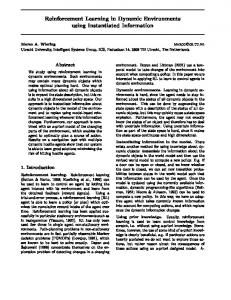
Section 2.2 outlines branch-and-bound algorithms, which constitute the core of our query processing. 2.1 The Time Parameterized R-Tree (TPR-Tree) The TPR-tree [Saltenis et al. 2000] is an extension of the R-tree that can answer prediction queries on dynamic objects. A dynamic object is represented with (i) a minimum bounding rectangle (MBR) that bounds its extents at the current time, and (ii) a velocity vector. Figure 1(a) shows the representation of two objects u and v, and that of the node that contains them. The arrows indicate the velocity directions for each edge, while the numbers correspond to their values. Velocities towards the negative direction of a coordinate axis are negative. Notice that different edge velocities will cause an object to grow (e.g., object v) or shrink with time. Similarly, an intermediate entry also stores a MBR and its velocity vector. As in traditional R-trees, the MBR tightly encloses all entries in the node at the current time (see node E in Figure 1(a)). The velocity vector is determined as follows: (i) the velocity of the right (upper) edge is the maximum of all velocities on the x- (y-) dimension in the subtree, and (ii) the velocity of the left (lower) edge is the minimum of them. This ensures that the MBR always encloses the underlying objects, but it is not necessarily tight. Figure 1(b) shows u, v and the enclosing node E at time 1 (observe how the extents and positions of u, v, E change). Since the upper edge of E moves with speed 2 (the speed of the upper edge of v) the MBR of E is not tight. Future MBRs (for example, in Figure 1(b)) are not stored explicitly, but are computed based on the current extents and velocity vectors. The TPR-tree answers instantaneous queries at some future time, for example, retrieve the objects that will intersect the query window at time 1 in Figure 1(b). Such queries are processed in exactly the same way as in the R-tree, except that the extents of the MBRs at the query time are first calculated dynamically and then compared with the query window. Node E must be visited because its computed MBR intersects the query, although its MBR at the current time does not. An improved TPR-tree with enhanced update policies is presented in Saltenis and Jensen [2002]. ACM Transactions on Database Systems, Vol. 28, No. 2, June 2003.


•

105

Fig. 2. Pruning metrics.

2.2 Branch-and-Bound (BaB) Algorithms The first R-tree BaB algorithm was proposed in Roussopoulos et al. [1995] for nearest neighbor (NN) queries. The algorithm introduces two distance metrics (both defined on intermediate entries) for pruning the search space. The first metric, mindist, is the minimum distance between the query object q and any object that can be in the subtree of entry E. The second metric, minmaxdist, refers to the minimum distance from q within which an object in the subtree of E is guaranteed to be found. Figure 2(a) illustrates these two metrics on the MBRs of E1 and E2 with respect to a query q. The algorithm of Roussopoulos et al. [1995] answers a NN query by traversing the R-tree in a depth-first (DF) manner. Specifically, starting from the root, all entries are sorted according to their mindist from the query point, and the entry with the lowest value is visited first. The process is repeated recursively until the leaf level where the first potential nearest neighbor is found. During backtracking to the upper levels, the algorithm only visits entries whose mindist is smaller than the distance of the nearest neighbor already found. As an example consider the R-tree of Figure 3, where the number in each entry refers to the mindist (for intermediate entries) or the actual distance (for point objects) from the query point (these numbers are not stored but computed dynamically during query processing). DF first visits the node of root entry E1 (since it has the minimum mindist), and then the node of E4 , where the first candidate object (a) is retrieved. When backtracking to the previous level, entries E 5 and E6 are excluded because their mindist is equal to or greater than the distance of a, and DF backtracks again to the root level. Then, it visits the nodes of E2 and E8 , where the actual NN (point h) is found. Minmaxdist (and other similar bounds) can be applied to further improve the performance. The DF approach was shown to be suboptimal in Papadopoulos and Manolopoulos [1997], which reveals that an optimal NN search algorithm only needs to visit those nodes whose MBRs intersect the so-called “search region”, that is, a circle centered at the query point with radius equal to the distance between the query and its nearest neighbor (shaded circle in Figure 3). A best-first (BF) algorithm for NN processing using R-trees is proposed in Hjaltason and Samet [1999]. BF keeps a heap with the entries of the nodes visited so far. Initially the heap contains the entries of the root sorted according to their mindist, and the algorithm processes the entries in ascending order of ACM Transactions on Database Systems, Vol. 28, No. 2, June 2003.

106

•


Fig. 3. Example of BaB algorithms.

their mindist. In Figure 3, when E1 is visited, it is removed from the heap and the entries of its node (E4 , E5 , E6 ) are added together with their mindist. The next entry visited is E2 (its mindist is currently the minimum in the heap), followed by E8 , where the actual result (h) is found and the algorithm terminates, because the mindist of all entries in the heap is greater than the distance of h. BF is optimal in the sense that it only visits the nodes necessary for obtaining the nearest neighbor. Both BF and DF can be easily extended for the retrieval of k nearest neighbors (kNN). Furthermore, BF is incremental, meaning that having retrieved the k NN, the k +1-th neighbor can be computed with minimal overhead. The BaB framework also applies to closest pair queries that find the pair of objects from two datasets, such that their distance is the minimum among all pairs. Corral et al, [2000] propose various algorithms based on the concepts of DF and BF traversal. The difference from NN is that the algorithms access two index structures (one for each data set) simultaneously. Mindist is now defined as the minimum distance between two objects that can lie in the subtrees of two intermediate entries (see Figure 2(b)). If the mindist of two intermediate entries E1 and E2 (one from each R-tree) is already greater than the distance of the closest pair of objects found so far, the subtrees of E1 and E2 cannot contain a closest pair. 3. TIME-PARAMETERIZED (TP) QUERIES The output of a spatio-temporal TP query has the general form hR, T, Ci, where R is the set of objects satisfying the corresponding instantaneous query (i.e., current result), T is the expiry time of R, and C the set of objects that will affect R at T. From the set of objects in the current result R, and the set of objects C that will cause changes, we can incrementally compute the next result. We refer to R as the conventional, and (T, C) as the time-parameterized component ACM Transactions on Database Systems, Vol. 28, No. 2, June 2003.


•

107

Fig. 4. Deriving TINF (o, q).

of the query. The result of a spatial query changes in the future because some objects “influence” its correctness. We denote the influence time of an object o with respect to a query q as TINF (o, q). The expiry time of the current result is the minimum influence time of all objects. Therefore, the time-parameterized component of a TP query can be reduced to a nearest neighbor problem by treating TINF (o, q) as the distance metric: the goal is to find the objects (C) with the minimum TINF (T). These are the candidates that may generate the change of the result at the expiry time (by adding to or deleting from the previous answer set). The above discussion serves as a high-level abstraction that establishes the close connection between the TP retrieval and NN search. In the sequel we study in detail TP versions of various spatial queries. 3.1 The TP Window Query (TP WQ) In order to find the influence time TINF (o, q) of an object o with respect to a query window q, we need the intersection period [Ts , Te ) during which o will intersect q. Figure 4(a) illustrates an example with a dynamic query q, and three dynamic objects u, v, w (the current time is 0). Figures 4(b) and 4(c) show the situations at time 1 and 3, respectively.1 The intersection period of object u is [0, 1), of v is [1, 3), while that of w is [∞, ∞) (i.e., w will never be part of the result). Notice that depending on the values of the two different velocities on a dimension, it is possible that some objects (e.g., w) may disappear (i.e., two opposite sides of the rectangle will meet) in the future (time 1). Such objects should be taken into account during query processing, since they will not affect the result after their disappearance. In general, (i) if an object o currently intersects the query window, TINF (o, q) = Te (i.e., TINF is the time that o will stop intersecting) or (ii) if o currently does not intersect the query window, TINF (o, q) = Ts (i.e., TINF is the time that o will start intersecting). Algorithms for computing the intersection periods, taking object disappearances into account, can be found in Saltenis et al. [2000] and Tao and Papadias [2002]. In order to avoid the computation of intersection periods for all data objects, we take advantage of the underlying R-tree (for static data) or TPR-tree (for 1 For

simplicity of illustration, we often use static 2D objects, while the extension to mobile objects and higher dimensions, unless explicitly stated, is straightforward. ACM Transactions on Database Systems, Vol. 28, No. 2, June 2003.

108

•


Fig. 5. Deriving TINF (E, q) when E intersects q.

dynamic data). Specifically, the tree is traversed in a top-down manner and intermediate entries that may not contain objects influencing the result before its expiration (i.e., the minimum TINF found so far) are immediately pruned; only qualifying entries (i.e., possibly containing the object with the minimum TINF ) are accessed. The influence time TINF (E, q) of a nonleaf entry E is defined in a way similar to mindist in NN search: TINF (E, q) is the lower bound of the influence time of any object that may lie in the subtree of E. If the MBR of E does not currently intersect q, TINF (E, q) is the time in the future that E starts to intersect q, because it is also the earliest time when any of the objects inside E can intersect (influence) q. If E intersects q at the current time, we need to distinguish two cases where (i) E is contained in q, or (ii) E partially intersects or contains q. Figure 5 illustrates these two cases with static objects u, v, their parent entry E (also static), and a dynamic query q. For the first case (Figure 5(a)), TINF (E, q) is set to the time (=1) that E starts to partially intersect q because, before this time, all objects in E are always contained in q, and hence do not influence the query result (1 is also the influence time of u). For the second case (Figure 5(b)), however, TINF (E, q) must be set to 0 because some object inside E (e.g., v) may influence the result as soon as the query moves. Summarizing, given the intersection period [Ts , Te ) of E and q, we define TINF (E, q) as follows: — TINF (E, q) = Ts , if q does not intersect E at the current time (i.e., Ts 6= 0), or — TINF (E, q) = 0, if q intersects, but does not contain, E at the current time, or — TINF (E, q) = TPI (E, q), if q contains E at the current time, where TPI (E, q) is the time that E starts to partially intersect q in the future (see Tao and Papadias [2002] for its computation). Having defined TINF for leaf and intermediate entries, we can employ any BaB algorithm to find the objects o with the minimum influence time TINF (o, q), which is exactly the expiry time of the TP query. As discussed in Section 2, BaB algorithms can be classified in two broad categories: depth- and best-first search. Figure 6(a) shows the pseudo-code of DF and Figure 6(b) for BF. In order to obtain the current result (R), both algorithms visit entries that intersect the original window even though the TINF of these entries maybe greater than the ACM Transactions on Database Systems, Vol. 28, No. 2, June 2003.


•

109

Fig. 6. BaB algorithms for time-parameterized window queries.

minimum influence time (T). Furthermore, we need to distinguish between (i) TINF (o, q) < T and (ii) TINF (o, q) = T. In the first case, o becomes the only object that influences the result so far, while in the second case o is added to the set of influencing objects C (i.e., it is possible that multiple objects will enter or exit the query window at the same time). 3.2 The TP k-Nearest Neighbor Query (TP k NN) We first consider single nearest neighbor (TP NN) queries before extending the solution to an arbitrary number k of neighbors. As before, our analysis focuses on deriving the metrics TINF (o, q) and TINF (E, q). Let q.NN be the current nearest neighbor of q. The influence time TINF (o, q) of an object o is the earliest time t in the future such that o(t) starts to get closer to q(t) than q.NN(t), where q.NN(t), o(t), q(t) are the positions of q.NN, o, q at time t, respectively. In general, TINF (o, q) is the minimum t that satisfies the following condition2 : ko(t), q(t)k ≤ kq.NN(t), q(t)k and t ≥ 0. If (o1 , . . . , on ) are the coordinates, and (o.V1 , . . . o.Vn ) the velocities of a moving point o on dimensions i = 1, . . . , n (similarly for q and q.NN), the above inequality can be transformed into the standard form At2 + Bt + C ≤ 0, where: A =

n X £

¤ (o.Vi − q.Vi )2 − (q.NN.Vi − q.Vi )2 ,

i=1

B = C =

n X i=1 n X

2[(oi − qi )(o.Vi − q.Vi ) − (q.NNi − qi )(q.NN.Vi − q.Vi )], and £

(oi − qi )2 − (q.NNi − qi )2

¤

i=1

2 ka, bk

denotes the Euclidean distance between points a and b. Other metrics can also be applied. ACM Transactions on Database Systems, Vol. 28, No. 2, June 2003.

110

•


Fig. 7. TINF for intermediate entries.

The solution is straightforward and omitted. If no t satisfies the inequality, TINF (o, q) is set to ∞, indicating that object o will never become closer to q than q.NN. In case of intermediate entries, TINF (E, q) indicates the earliest time when some object in the subtree of E may start to be closer to q (than q.NN). This is illustrated in Figure 7(a), where q.NN and MBR E are static and q is moving east. At time 2, the mindist of E to q becomes shorter than kq.NN, qk, which implies that some object in E may start to get closer to q (i.e., TINF (E, q) = 2). More formally, TINF (E, q) is the minimum t that satisfies the condition: mindist(E(t), q(t)) ≤ kq.NN(t), q(t)k and t ≥ 0. This inequality requires case-by-case discussion because the computation of mindist(E(t), q(t)) depends on the relative positions of E and q. Figure 7(b) illustrates an example where the MBR E (corner points a, b, c, d ) is static and the query point is moving along line l . Before q reaches point e, mindist(E, q) should be calculated with respect to point a. When q is on the line segment ef, mindist is the distance from q to edge ab of E. Similarly, after q passes points f , g , and h, mindist should be computed with respect to point b, edge bc, and point c, respectively. Benetis et al. [2002] provide an algorithm for obtaining mindist(E(t), q(t)), covering also the case where MBR E is dynamic and the dimensionality is higher. The extension to TP kNN queries is straightforward. The only difference is that now the influence time of an object o corresponds to the earliest time that o starts to get closer to q than any of the k current neighbors. Specifically, assuming that the k current neighbors are q.1NN, q.2NN, . . . , q.kNN, we first compute the influence time TINFi of o with respect to each q.iNN (i = 1, 2, . . . , k) following the previous approach. Then TINF (o, q) is set to the minimum of TINF1 , TINF2 , . . . , TINFk . Similarly, for TINF (E, q) we first compute the TINFi of E with respect to each q.iNN and then set TINF (E, q) to the minimum of TINF1 , TINF2 , . . . , TINFk . Figure 8 illustrates the pseudo-code of the DF algorithm for TP kNN queries (the BF code can be obtained in a way similar to Figure 6(b)). Notice that, unlike TP WQ queries where the conventional R and the time-parameterized components (T, C) can be obtained in one pass, TP kNN processing requires the retrieval of R (using a regular NN algorithm, e.g., Roussopoulos et al. [1995] and Hjaltason and Samet [1999]) before T and C, since the objects that influence the result depend on the current nearest neighbors. ACM Transactions on Database Systems, Vol. 28, No. 2, June 2003.


•

111

Fig. 8. Depth-first algorithm for time-parameterized kNN queries.

Fig. 9. Influence time of object pairs.

3.3 The TP Spatial Join (TP SJ) A spatial join returns all pairs of objects from two datasets that satisfy some spatial predicate (e.g., intersection). The join result changes in the future when: (i) a pair of objects in the current result, ceases to satisfy the join condition, or (ii) a pair not in the result starts to satisfy the condition. Figure 9(a) shows an example of TP join. Objects A3 and B2 , which do not intersect at the current time, will start intersecting at time 1, hence influencing the result. In general, we denote the influence time of a pair of objects (o1 , o2 ) as TINF (o1 , o2 ). Figure 9(b) lists TINF for all pairs of objects. The influence time is ∞, if a pair will never change the join result (e.g., (A2 , B2 )). The expiry time is the minimum influence time (i.e., TINF (A3 , B2 ) = 1). As in the other types of TP queries, by adding or deleting the pair of objects that causes the change, the join result is updated incrementally. A TP join can be regarded as a closest pair (CP) query (see Section 2.2) by treating TINF (o1 , o2 ) as the distance metric between objects o1 and o2 . In addition, we also need to define TINF (E1 , E2 ) to replace mindist(E1 , E2 ) (see Figure 2(b)), where TINF (E1 , E2 ) should be a lower bound of the TINF (o1 , o2 ) of ACM Transactions on Database Systems, Vol. 28, No. 2, June 2003.

112

•


Fig. 10. Algorithm for time-parameterized spatial join.

any two objects o1 and o2 in the subtrees of E1 and E2 , respectively. The analysis of TINF (o1 , o2 ) and TINF (E1 , E2 ) is very similar to that for TP window queries and we simply summarize the definitions: — TINF (o1 , o2 ) = Te , if Ts = 0 (i.e., o1 and o2 currently satisfy the join condition), or TINF (o1 , o2 ) = Ts , if Ts > 0 (i.e., o1 and o2 do not satisfy the condition), where [Ts , Te ) is the intersection period of objects o1 and o2 — TINF (E1 , E2 ) = Ts , where Ts is the starting point of the intersection period [Ts , Te ) of E1 and E2 (unlike TP window queries, this case also includes containment) Figure 10 presents the algorithm for TP join queries, which obtains R, T and C in a single pass. To achieve this, the algorithm traverses the R- (or TPR-) trees for the two datasets simultaneously. For a pair of nonleaf entries (E1 , E2 ), their subtrees are explored if one of the following conditions holds: (i) the MBRs of E 1 and E2 intersect (so some objects in their subtrees may satisfy the join condition), or (ii) TINF (E1 , E2 ) is less than the minimum influence time of all object pairs found so far (in this case their subtrees may contain object pairs that trigger the next result change). For simplicity, the algorithm assumes that the two index structures have the same height; trees of different heights can be handled by the techniques proposed in Corral et al. [2000]. 4. CONTINUOUS WINDOW QUERIES AND SPATIAL JOINS Similar to TP variations, every traditional spatial query has a continuous counterpart, which returns a set of tuples {hR1 , T1 i, hR2 , T2 i, . . . , hRm , Tm i}, such that Ri (1≤ i ≤ m) is the result during (future) time interval Ti , where m is the total number of result changes. A continuous query can be answered by repetitive execution of TP queries until some termination clause is satisfied. To illustrate, consider the continuous window query (CWQ) in Figure 11(a), where the goal is to “find the gas stations within 5 km during my trip from s to e, via intermediate point p”. We start by performing the first TP WQ (NOTE: The query window is circular) at s, which returns R1 = Ø (i.e., no station is in the range currently), the expiry time T1 = s1 (i.e., at this point ACM Transactions on Database Systems, Vol. 28, No. 2, June 2003.


•

113

Fig. 11. Examples of spatio-temporal continuous queries.

station a starts to qualify), and the change C1 = {a}. Then, a separate TP WQ query is executed at the expiry point (T1 = s1 ), returning R2 = {a}, T2 = s2 , C2 = {−a} (indicating that a ceases to qualify at s2 ). This process is repeated until the entire path is completed, obtaining the final result {hØ, [s, s1 )i, h{a}, [s1 , s2 )i, hØ, [s2 , s3 )i, h{b}, [s3 , s4 )i, . . .}. This repetitive approach can be applied to other continuous queries. Figure 11(b) shows an example for continuous kNN (CkNN): “find my nearest gas stations during my trip from s to e”. By executing three TP NN queries (at positions s, s1 , s2 respectively), we retrieve the result {h{a}, [s, s1 )i, h{b}, [s1 , s2 )i, h{c}, [s2 , e)i}, meaning that a will be the NN during [s, s1 ), b during [s1 , s2 ) and so on. Following the same idea, it is straightforward to derive the corresponding repetitive algorithm for continuous spatial joins (CSJ). The repetitive approach is output sensitive because the number of TP queries equals the number of result changes. Observe that, however, except for the first TP query, the subsequent ones do not need to retrieve all the R, T, C components. For example, the second TP only needs to return T2 and C2 , while R2 can be obtained by applying C1 to the previous result R1 . Acquiring only T2 and C2 can be much cheaper than also retrieving R2 , which involves significantly more information (especially for joins). In general, subsequent TPqueries only need to return the time-parameterized components (Ti , Ci ) while the query result Ri can be maintained by applying the changes Ci incrementally. Motivated by this, we develop single-pass algorithms that answer continuous queries with a single traversal of the underlying index. We first discuss CWQ and CSJ, which can be solved with the same methodology. As mentioned earlier, the influence time of an object (or a pair of objects) in TP WQ (or TP SJ) does not depend on the current result. Consider the continuous WQ in Figure 12(a) that retrieves the results until time 4 (assuming current time 0). Here, we define two influence times TINFs , TINFe for each object o because it may change the result at most twice. Specifically, (i) for an object (e.g., d ) that is currently disjoint with q, its TINFs equals the time (i.e., 2) that it intersects q in the future, while its TINFe corresponds to the time (i.e., 6) that it becomes disjoint with q again after TINFs . (ii) If an object (e.g., b) satisfies q, then its TINFs is the time (i.e., 1) when it falls out of q, while its TINFe is set to ∞ (i.e., it will not influence the result after TINFs ). As with TP queries, some objects (e.g., a and c) may never affect the result, and their TINFs and TINFe are both ∞. ACM Transactions on Database Systems, Vol. 28, No. 2, June 2003.

114

•


Fig. 12. Influence time of continuous queries.

Fig. 13. Algorithms for continuous window queries and spatial joins.

Retrieving the result changes is equivalent to returning the objects in ascending order of their influence time, except that both TINFs and TINFe should be considered. In Figure 12(a), for example, the sequence of changes is −b (remove b from the result), d (i.e., add d into the result), e, −d − e (i.e., d and e are removed simultaneously), at time 1, 2, 3, and 6, respectively. Since the query considers only up to time 4, the final result contains the first 3 changes. Thus, a CWQ can be answered with incremental kNN retrieval (see Section 2.2), by treating TINFs and TINFe as distance metrics. Figure 13(a) illustrates the pseudo-code, where the influence time of a nonleaf entry is derived in the same way as TP queries. The algorithm is essentially a BF (incremental) variation of kNN search, where the value of k is not known ACM Transactions on Database Systems, Vol. 28, No. 2, June 2003.


•

115

in advance. It is worth mentioning that, an alternative approach to process the continuous query in Figure 12(a) is to retrieve all the objects intersecting the “extended” region (the bold rectangle) covering the area swept by q up to time 4, and then sort the returned objects by their influence time. This method, however, does not support other termination clauses. For example, if the clause asks to stop after a certain number of changes, then the extended region cannot be computed. Our algorithm, on the other hand, retrieves objects in ascending order of their influence time and supports arbitrary termination conditions. The continuous spatial join can be reduced to incremental closest pair retrieval in a similar manner. Each pair of objects also defines two influence time TINFs and TINFe : (i) for two objects that currently intersect, their TINFs equals the time in the future that they become disjoint and TINFe = ∞; (ii) if two objects are disjoint, then their TINFs (TINFe ) corresponds to the time when they start to intersect (or become disjoint again after TINFs ). Figure 12(b) shows the influence time (TINFs /TINFe ) for the example in Figure 9(b). The CSJ algorithm of Figure 13(b) returns object pairs in ascending order of their TINFs and TINFe . Continuous kNN queries, however, can not be processed with this method, since unlike WQ and SJ, the influence time in TP kNN depends on the current query result and objects’ influence time in the future will be modified as the nearest neighbors change. In the next section, we develop single-pass algorithms for CkNN queries in order to avoid the high overhead of the repetitive approach. 5. CONTINUOUS NEAREST NEIGHBORS Since for CkNN queries the objects’ influence period cannot be determined at the current time (which is a precondition for the algorithms of Figure 13), the following methods are inherently different from those for continuous window queries and joins. Furthermore, we assume that the user specifies a temporal termination condition, that is, given a moving point q at the current time 0 and a time limit TL, the CkNN query returns the k nearest neighbors of q at any time during [0, TL]; arbitrary termination conditions (e.g., after a specified number of result changes) are not supported. Section 5.1 elaborates the concrete algorithm for static data indexed by R-trees and Section 5.2 deals with moving data indexed by TPR-trees. 5.1 Ck NN Algorithm for Static Data For simplicity, we illustrate the concepts for single nearest neighbor retrieval and later discuss the extension to kNN for arbitrary values of k. Let s and e be the positions of moving query q at time 0 and TL, respectively; then, the trajectory of q during [0, TL] is line segment [s, e]. The split list SL contains a set of split points (where the NN of q changes), with the starting (s) and ending (e) points being the first and last elements in SL. In Figure 11(b), for example, SL consists of {s, s1 , s2 , e}. Let si and si+1 be two consecutive split points in SL (0 ≤ i < | SL |−1, where | SL | denotes its size); all positions in segment [si , si+1 ] have the same NN, denoted as si .NN. For instance, s1 .NN in Figure 11(b) is point a, ACM Transactions on Database Systems, Vol. 28, No. 2, June 2003.

116

•


Fig. 14. Updating the split list.

which is also the NN for all points in interval [s, s1 ]. In the sequel, we say that si .NN covers point si and interval [si , si+1 ] (e.g., a covers s and [s, s1 ]). To report all split (and the corresponding covering) points with a single traversal, we start with an initial SL that contains only two split points s and e with their covering points set to Ø (meaning that currently the NN of all points in [s, e] are unknown), and incrementally update the SL during query processing. At each step, SL contains the current result with respect to all the data points processed so far. The final result contains the split points that remain in SL after the termination together with their nearest neighbors. Processing a data point o involves updating SL, if o is closer to some point u ∈ [s, e] than its current nearest neighbor u.NN (i.e., if o covers u). An exhaustive scan of [s, e] (for points u covered by o) is intractable because the number of points is infinite. We observe that it suffices to examine whether o covers any split point currently in SL, as described in the following lemma. LEMMA 5.1. Given a split list SL {s0 , s1 , . . . , s|SL|−1 } and a new data point o, o covers some point on query segment q if and only if o covers a split point. As an illustration of Lemma 5.1, consider Figure 14(a) where the data points a, b, c, d are processed in alphabetic order. Initially, SL = {s, e} and the NN of both split points are unknown. Since a is the first point encountered, it becomes the current NN of every point in q, and information about SL is updated as s.NN = e.NN = a. The circle centered at s (e) with radius ks, ak(ke, ak) is called the vicinity circle of s (e). When processing the second point b, we only need to check whether b is closer to s and e than their current NN, or equivalently, whether b falls in their vicinity circles. The fact that b is outside both circles indicates that every point in [s, e] is closer to a (due to Lemma 5.1); hence, we ignore b and continue to the next point c. In Figure 14(b), since c falls in the vicinity circle of e, a new split point s1 is inserted to SL; s1 is the intersection between the query segment and the perpendicular bisector of segment [a, c], meaning that points to the left of s1 are closer to a, while points to the right of s1 are closer to c. The NN of s1 is set to c, indicating that c is the NN of points in [s1 , e]. Finally, point d does not update SL because it does not cover any split point (notice that d falls in the circle of e in Figure 14(a), but not in Figure 14(b)). Since all points have been ACM Transactions on Database Systems, Vol. 28, No. 2, June 2003.


•

117

Fig. 15. Pruning non-qualifying entries.

Fig. 16. Sequence of accessing entries.

processed, the split points that remain in SL determine the final result (i.e., {ha, [s, s1 ]i, hc, [s1 , e]i}). The above general methodology can be used for arbitrary dimensionality, where perpendicular bisectors and vicinity circles become perpendicular bisectplanes and vicinity spheres. Its application for processing nonindexed datasets is straightforward, that is, the input dataset is scanned sequentially and each point is processed, continuously updating the split list. As with the previous query types, however, CNN processing can be significantly accelerated by employing R-trees and the branch-and-bound technique to prune the search space. In particular, intermediate entries can be excluded from search based on the following observation: Given an intermediate entry E and query segment q, the subtree of E must be searched if and only if there exists a split point si ∈ SL such that ksi , si .NNk > mindist(si , E). Figure 15 shows a query segment q = {s, e}, where the current SL that contains three split points s, s1 , e (s.NN = a, s1 .NN = e.NN = b). Rectangle E represents the MBR of an intermediate node. Since ks, ak < mindist(s, E), ks1 , bk < mindist(s1 , E) and ke, bk < mindist(e, E), entry E will not be visited because it cannot contain any point closer to the query than the existing nearest neighbors (i.e., E is outside all vicinity circles). The order of entry accesses is very important for avoiding unnecessary visits. Consider, for example, Figure 16(a) where points a and b have been processed, whereas entries E1 and E2 have not. Both E1 and E2 are qualifying entries, meaning that they must be accessed according to the current status of SL. Assume that E1 is visited first, the data points c, d in its subtree are processed, ACM Transactions on Database Systems, Vol. 28, No. 2, June 2003.

118

•


Fig. 17. Processing steps of the CNN algorithm.

and SL is updated as shown in Figure 16(b). After the algorithm returns from E1 , the MBR of E2 is pruned from further exploration since ksi , si .NNk < mindist (si , E2 ) for each split point si . On the other hand, if E2 is accessed first, E1 must also be visited. To minimize the number of node accesses, qualifying entries are accessed in increasing order of their minimum distances to the query segment q. The above discussion is directly applicable to CkNN (k > 1) queries except that, ksi , si .NNk should be replaced with the distance ksi , si .kNNk from si to its kth (i.e., farthest) NN (we consider that a change in the order of existing neighbors does not constitute a result change). Thus, the pruning process is the same as single-neighbor queries. The handling of leaf entries is also similar. Specifically, a data object o is processed in a two-step manner. The first step identifies the set of split points si that are covered by o (i.e., ksi , ok < ksi , si .kNNk). If no such split point exists, o is ignored (i.e., it cannot be one of the kNN of any point on q). Otherwise, the second step updates the split list, by inserting new split point(s) and, possibly, removing some old ones (for details, see Tao et al. [2002]). Both the DF and BF traversal paradigms can be applied for CkNN. For simplicity, we elaborate the algorithm using depth-first traversal for the query of Figure 17(a) (single NN). The split list SL is initiated with two entries {s, e}, the root of the R-tree is retrieved and its entries are sorted by their distances to segment q. Since the mindist of both E1 and E2 are 0, one of them is chosen (e.g., E1 ), its child node is visited, and the entries inside it are sorted (order E4 , E 3 ). The node of E4 is accessed, points f, d, g are processed according to their distances to q, and f becomes the first NN of s and e (Figure 17(a)). ACM Transactions on Database Systems, Vol. 28, No. 2, June 2003.


•

119

Fig. 18. Algorithm for obtaining influence period of an object.

The next point g covers e and adds a new split point s1 to SL (Figure 17(b)). Point d does not incur any change because it does not cover any split point. Then, the algorithm backtracks to the upper level and visits the subtree of E3 . At this stage, SL contains four split points (Figure 17(c)). Now the algorithm backtracks to the root and then follows entries E2 , E6 ), where SL is updated again (note the position change of s1 ) (Figure 17(d)). Since E5 falls out of all vicinity circles, it is pruned and the algorithm terminates with the final result: {hk, [s, s1 ]i, h f , [s1 , s2 ]i, h g , [s2 , e]i}. 5.2 Ck NN on Volatile Data For CkNN queries on volatile data, the split list SL consists of a set of split timestamps3 ti (0 ≤ i ≤ | SL | − 1), such that the k nearest neighbors of q during each interval [ti , ti+1 ] (⊆[0, TL], the query interval) are the same, denoted as Ri = {ti .1NN, . . . , ti .kNN}. Initially SL contains only two timestamps 0 and TL (the time limit specified by the query), and is updated during the traversal of the index (TPR-tree). Specifically, when a leaf object o is encountered, the algorithm checks if there exists any time t ∈ [ti , ti+1 ] (for all 0 ≤ i ≤ |SL| − 1) when o is closer to q than some ti . j NN(1 ≤ j ≤ k). Similar to Lemma 5.1, for this purpose, it suffices to consider only the split timestamps: following the same terminology, we say that a data point o covers split timestamp ti , if kq(ti ), o(ti )k < kq(ti ), ti . j NN(ti )k for any 1 ≤ j ≤ k. The distance ko, qk between o and q can be represented as a function of time t: At2 + Bt + C, where A, B, C are constants dependent on the positions and velocities of o and q. Thus, deciding if o covers a split timestamp ti involves solving a set of inequalities, as shown in Figure 18, which returns an influence period ti .[α j , β j ] ∪ ti .[γj , δj ] for each NN ti . j NN(0 ≤ i ≤ |SL| − 1, 1 ≤ j ≤ k) during which o is closer to q than ti . j NN. Object o is ignored, if it does not cover any current split timestamp, or equivalently, all influence periods are empty (i.e., ti .[α j , β j ] = ti .[γ j , δ j ] = Ø, for all 0 ≤ i ≤ |SL| − 1, 1 ≤ j ≤ k). Otherwise, o influences the query result and SL is updated using the algorithm shown in Figure 19, which essentially computes the kNNs of the query point at the starting and ending timestamps of each nonempty influence period. Since these are the only timestamps where changes of nearest neighbors may occur, we do not need to consider the other timestamps. 3 Note

that ti corresponds to split point si in the static case. We use different symbols to emphasize that ti and si are temporal and positional separators, respectively. ACM Transactions on Database Systems, Vol. 28, No. 2, June 2003.

120

•


Fig. 19. Algorithm for updating SL.

Fig. 20. Algorithm for CkNN queries (volatile data).

As with the static case, CkNN queries on dynamic objects can be significantly accelerated with a TPR-tree. Specifically, given a (moving) MBR E of a nonleaf entry, E is pruned if it cannot come closer to q than any of its current nearest neighbors. Qualifying entries are processed in ascending order of their minimum mindist during the interval [0, TL]. The complete algorithm for volatile objects is presented in Figure 20, where the computation of line 10 is described in Benetis et al. [2002]. It is worth mentioning that the algorithm in Figure 20 generalizes the method of Benetis et al. [2002] in several ways. First, it supports kNN retrieval, including the influence period computation and a new SL updating method. Second, it contains the mechanism (the algorithm in Figure 19) of removing redundant split points (recall from Figure 17 that the number of split points may actually decrease during the process), resulting in higher efficiency. As shown in the experimental evaluation, the single-pass algorithm outperforms the repetitive approach (i.e., issuing multiple TP queries), at the tradeoff of lower applicability. Specifically, the repetitive method outputs changes in ACM Transactions on Database Systems, Vol. 28, No. 2, June 2003.


•

121

chronological order, and can be applied to various termination conditions (e.g., finish after 10 NN changes) not supported by the single-pass approach, where the termination time limit TL must be specified in advance. 6. PERFORMANCE ANALYSIS This section analyzes the performance of TP and continuous algorithms by deriving cost models that predict the query cost (in terms of the number of node accesses) with R- and TPR-trees (indexing static and mobile objects, respectively). Given a 2D moving rectangle o with current MBR {o1L , o1R , o2L , o2R } and velocities as {o.V1L , o.V1R , o.V2L , o.V2R }, we call oi R − oiL (o.Vi R − o.ViL ) its spatial (velocity) extent on the ith dimension. We start with the preliminary case, where (i) each object has fixed spatial (velocity) extent s(sV ) on all dimensions, (ii) the location oiL of its left boundary (on each dimension) uniformly distributes in [0, 1 − s], and (iii) the velocity o.ViL of the boundary is also uniform in [Vmin , Vmax − sV ], where Vmin and Vmax are constants denoting the minimum and maximum velocity values, respectively. The definitions for point data are similar, except that the spatial and velocity extents are zero; thus, we abbreviate their location and velocities as {o1 , o2 } and {o.V1 , o.V2 }. The results of the preliminary case can be extended to nonuniform data with variable spatial/velocity extents using histograms, as discussed later. Our analysis utilizes the following lemmas: LEMMA 6.1 (R-TREE NODE EXTENTS) [THEODORIDIS AND SELLIS 1996]. Let N static rectangles that distribute uniformly in the data space and have identical extents s. Then, the MBRs of the ith level of the resulting R-tree (0 ≤ i ≤ h − 1, where h is the tree height) also follow uniform distribution, and their extents on each dimension are si = (Di+1 · f i+1 /N )1/2 , where f is the average node fanout 1/2 and Di+1 = [1 + (Di − 1)/ f 1/2 ]2 with D0 = s2 · N . LEMMA 6.2 (TPR-TREE NODE EXTENTS) [SALTENIS ET AL. 2000]. Consider N moving 2D rectangles whose spatial (velocity) extents uniformly distribute in the unit data space [0, 1]2 (velocity space [Vmin , Vmax ]2 ). Then, the MBRs (VBRs) of the ith level of the resulting TPR-tree also follow uniform distribution in the data (velocity) space, and their extents on each dimension are si = [(Vmax − Vmin )2 · f i+1 · H 2 /3N ]1/4 (sV i = 31/2 · si /H), where f is the average node fanout and H is the horizon parameter of the TPR-tree (specifying how far into the future the tree is optimized for).4 LEMMA 6.3 (INTERSECTION PROBABILITY OF TWO MOVING RECTANGLES) [TAO ET AL. 2003]. Consider a moving rectangle q with current MBR {q1L , q1R , q2L , q2R } and velocities {q.V1L , q.V1R , q.V2L , q.V2R }, and another rectangle with spatial (velocity) extent s (sV ) that uniformly distributes in the data (velocity) space [0, 1]2 ([Vmin , Vmax ]2 ). The probability Pintr (q, s, sV , t) that the two rectangles 4 This

result holds for bulk-loaded TPR-trees. To the best of our knowledge, however, there does not exist any technique that can provide accurate estimation for incremental TPR-trees. Performance analysis on nonuniform data is not available either. Our analysis, on the other hand, is independent of the node extent estimation of the underlying index. ACM Transactions on Database Systems, Vol. 28, No. 2, June 2003.

122

•

Y. Tao and D. Papadias Table I. Frequently Used Symbols

Symbol N {o1L , o1R , o2L , o2R } {o.V1L , o.V1R , o.V2L , o.V2R } PINF (t)

Description dataset cardinality spatial MBR of a rectangle o velocity MBR of a moving rectangle o probability that the influence time of an object is before t probability that the influence time of a moving object is before t, when its velocities take specific values probability that the expiry time is before t expected expiry time spatial extent of a rectangle velocity extent of a rectangle spatial extent of a level-i node of the R-(TPR-) tree velocity extent of a level-i node of the TPR-tree the time limit specified by a continuous query

PINF 0 (t)

PT (t) ET s sV si sV i TL

intersect during the future time interval [0, t] is: µ Pintr (q, s, sV , t) =

1 Vmax − Vmin − sV

¶2

Vmax Z −sV Vmax Z −sV

Vmin

ASR (q 0 , t) dV1 dV2

Vmin

where ASR (q 0 , t) is the area covered during the future interval [0, t] by a moving rectangle q 0 with MBR {q1L − s, q1R , q2L − s, q2R } and velocities {q.V1L − V1 − sV , q.V1R − V1 , q.V2L − V2 − sV , q.V2R − V2 }. If the MBR (VBR) of q is unknown but its spatial (velocity) extent equals qs (qsV ), then the probability Pintr (qs , qsV , s, sV , t) is: Pintr (qs, qsV , s, sV , t) ¶2 µ ¶2 µ 1 1 = Vmax − Vmin − sV Vmax − Vmin − qsV Vmax −qs V −qs V −s V −s V max V max V max Z Z Z Z V ¡ ¢ ¡ ¢ ¡ ¢ ¡ ¢ ASR (q 0 , t) d V1 d V2 d qV1 d qV2 , Vmin

Vmin

Vmin

Vmin

0

where q is an MBR with spatial extent s + qs and velocities {qV1 − V1 − sV , qV1 + qsV − V1 , qV2 − V2 −sV , qV2 + qsV − V2 }. Table I lists the frequently used symbols. 6.1 Analysis for TP and Continuous Window Queries As discussed in Section 3.1, the result of a TP WQ expires when (i) an object not intersecting query q at the current time, intersects q in the future or (ii) an object that satisfies q now stops qualifying later. To derive the expected expiry time ET , we need to compute the probability PINF (t) that the influence time ACM Transactions on Database Systems, Vol. 28, No. 2, June 2003.


•

123

Fig. 21. Deriving PINF for static objects.

TINF (o, q) of an object o is before t. Focusing on static point data, Figure 21(a) shows the extents of q at time 0 (i.e., the current time) and t, respectively. Notice that TINF (o, q) ≤ t, if and only if point o falls into the validity region (VR), which is the convex hull of the vertices of q(0) and q(t) minus their intersection (shaded area in Figure 21(a)). For instance, since A is not in VR we can infer that TINF (A, q) > t, which is true because A remains in q during [0, t]. Similarly, we may assert that TINF (B, q) ≤ t; in fact, TINF (B, q) equals the time that B is swept by the upper edge of q, that is, when q is at the dashed rectangle. For uniform distribution and unit data space, PINF (the probability that a point lies in VR) equals the area AVR (q, t) of VR, or equivalently the area swept by the edges of q during interval [0, t]. The analysis of PINF for static rectangles can be reduced to static points. Assuming s to be the spatial extent of a data rectangle o, for a query q with current MBR {q1L , q1R , q2L , q2R } and velocities {q.V1L , q.V1R , q.V2L , q.V2R }, we formulate another query q 0 with MBR {q1L − s, q1R , q2L − s, q2R } (i.e., by enlarging q with length s), and the same velocities. Thus, q intersects o at time t, if and only if q 0 covers the lower-left corner of o at t. Figure 21(b) illustrates the transformed q 0 (0) and q 0 (t) (from q(0) and q(t), respectively), as well as the resulting VR (obtained from q 0 in the same way as in Figure 21(a)) that covers the lower-left corners of all rectangles whose influence time is before t (e.g., for rectangles A and B: TINF (A, q) ≤ t, TINF (B, q) > t). As with the point case, PINF (t) equals the area of VR for uniform distribution. Dynamic objects can also be reduced to static points. Let o be a 2D moving rectangle with current MBR {o1L , o1L + s, o2L , o2L + s} and velocities {o.V1L , o.V1L + sV , o.V2L , o.V2L + sV }. Given a query q with MBR {q1L , q1R , q2L , q2R } and velocities {q.V1L , q.V1R , q.V2L , q.V2R }, we formulate a 0 = qiL − s, qi0 R = qi R , and (ii) new query q 0 such that, for 1 ≤ i ≤ 2, (i) qiL 0 0 q .ViL = q.ViL − o.ViL − sV , q .Vi R = q.Vi R − o.ViL . Then, o intersects q at timestamp t, if and only if q 0 covers the static point {o1L , o2L } (i.e., the current lower-left corner of o) at t. The probability PINF 0 that the influence time of object o with specific velocity values {o.V1L , o.V1L + sV , o.V2L , o.V2L + sV } is earlier than t equals the area AVR (q 0 , t) of the resulting VR, where q 0 is derived from q as described earlier. It follows that the overall probability PINF (that TINF (o) ≤ t) ACM Transactions on Database Systems, Vol. 28, No. 2, June 2003.

124

•


Fig. 22. Deriving Pacs−i .

is the average PINF 0 over all possible values in [Vmin , Vmax ]: 1 PINF (t) = (Vmax − Vmin − sV )2

Vmax Z −sV Vmax Z −sV

PINF 0 (q 0 , t) d(o.V2L ) d(o.V1L )

Vmin

Vmin

with PINF 0 (q 0 , t) = AVR (qiL − S, qi R , q.ViL − o.ViL − sV , q.Vi R − o.ViL , t), for 1 ≤ i ≤ 2

(6.1)

where AVR is the area of the validity region. Since the expiry time is the earliest influence time of all objects, the probability PT (t) for the result to expire before t, equals the probability that the influence time of at least one object is smaller than t, or formally: PT (t) = 1 − (1 − PINF (t)) N ,

(6.2)

where N is the dataset cardinality and PINF (t) is given by Eq. 6.1. Taking the derivative of PT (t), we obtain its probability density function pT (t), after which the expected expiry time can be computed as: Z∞ ET = t · PT (t) dt. (6.3) 0

Having derived ET , we are now ready to study the query cost of TP WQ. A node is visited only if its MBR intersects q during [0, ET ]. Figure 22(a) illustrates an example for static data where A and B are nodes of an R-tree. The search region (SR) (shaded area) is defined by the convex hull of the vertices of q(0) and q(ET ). MBRs overlapping q(0) may contain objects in the conventional result R, while nodes intersecting the rest of the SR (other than q(0)) are necessary for retrieving the TP components T and C. To compute the access probability Pacs−i for a level-i node, observe that a MBR intersects SR, if and only if its lower-left corner lies in the extended search region (ESR), which is obtained by enlarging the original SR with si (see Figure 22(b)), where si is the spatial extent of the MBR. By Lemma 6.1, for uniform data the node MBR distribution is also uniform; thus, Pacs−i equals the area AESR (q, si ) of ESR (in a unit data space). Similarly, for TPR-trees (indexing moving objects), Pacs−i corresponds to the probability that query q intersects a moving MBR (of a level-i node) satisfying ACM Transactions on Database Systems, Vol. 28, No. 2, June 2003.


•

125

the following conditions (on each dimension): (i) its spatial (velocity) extent is si (sV i ), and (ii) the location (velocity) of its left boundary uniformly distributes in [0, 1 − si ] ([Vmin , Vmax − sV i ]). The solution of this problem can be obtained directly from Lemma 6.3. In particular, notice that the computation of AESR (q, si ) (i.e., the area of the enlarged search region shown in Figure 22(b)) is merely a special case of this problem, where Vmin = Vmax = 0. Formally, the number of node accesses of a TP WQ can be represented as: ¸ h−1 · X N NA(q) = Pacs−i (q, si , sVi , E T ) , (6.4) f i+1 i=0

where N is the dataset cardinality, f the average node fanout, h the height of the tree, si , sVi the spatial and velocity extents of a node at the ith level (sVi = 0 for R-trees). The estimation of si , sVi is shown in Lemmas 6.1 and 6.2 respectively, and Pacs−i (q, si , sVi , E T ) is computed as Pintr (q, s, sV , t) in Lemma 6.3. Compared with a traditional WQ returning only R, a TP WQ obtains the additional validity information T, C with marginal overhead. Consider, for instance, Figure 22(a) where a traditional query visits all nodes intersecting q(0); the TP WQ accesses an extra node (e.g., node B) if its MBR intersects SR but not q(0). The number of such nodes, however, is (as verified by the experimental evaluation) rather small because: (i) if the data density (or the cardinality) is high, the distance that a WQ travels before its result changes (e.g., a new object intersects the edge of the query window) is small; therefore, the extra SR (compared to q(0)) is minor. (ii) On the other hand, if the data density is low, nodes have large MBRs implying that a node intersecting SR also intersects q(0) with high probability, in which case it is visited by both the conventional and the TP window query. The performance analysis of continuous WQ follows the above discussion in a straightforward manner. Specifically given a time limit TL, the number of result changes is approximately TL/ET . The query cost can also be obtained using Eq. 6.4, except that ET should be replaced with TL in computing Pacs−i , because a node is visited if it intersects q during [0, TL], instead of [0, ET ]. 6.2 Analysis for TP and Continuous k NN Queries We first derive the expected expiry time ET , by starting with the single NN case (i.e., k = 1) before generalizing to multiple NN. In particular, we focus on deriving the probability PINF (t) that the influence time of an object o is earlier than time t, after which ET can be obtained using Eqs. 6.2 and 6.3. If q.NN is the current nearest neighbor of q, the influence time TINF (o, q) of o is the earliest time t in the future that ko(t), q(t)k = kq.NN(t), q(t)k. Let 2t be the circle that centers at q(t) with radius kq.NN(t), q(t)k. For static datasets, TINF (o, q) ≤ t if and only if point o falls in 2t but not 20 (the circle centering at q(0)). As a result, the validity region that contains all data points with influence time before t, is the extent of 2t minus the intersection between 2t and 20 . In Figure 23(a), for example, since point A lies in VR (i.e., the shaded area), we can infer that TINF (A, q) ≤ t, which is true because TINF (A, q) = t A < t (note that q(t A ) has ACM Transactions on Database Systems, Vol. 28, No. 2, June 2003.

126

•


Fig. 23. Deriving PINF for static data.

equal distances to q.NN and A). On the other hand, TINF (B, q) > t because B is outside VR. For uniform distribution, the probability that an object (other than q.NN) falls in VR (i.e., also the probability PINF (t) that the influence time of an object is before t) equals AVR /(1 − area(20 )), where AVR is the area of VR and the constant 1 denotes the area of the data space. Notice that the denominator captures the fact that there cannot be any object inside 20 . Since q.NN can be at various positions with different probabilities [Berchtold et al. 1997, Weber et al. 1998], the expected PINF (t) should consider all these positions, which results in excessively complex formulas. Instead, we follow a different approach, which, as evaluated in the experiments, provides satisfactory estimation. The motivation is that, for uniform distributions, the expected distance d 1 from a point to its NN equals r d1 =

1 π·N

[Bohm 2000, Berchtold et al. 2001], that is, there is exactly one point in the circle centering at the query with radius d 1 . Hence, we assume that the NN of q changes as soon as it comes within distance d 1 to a point other than q.NN. As a result, the area AVR of q VR (shown in Figure 23(b)), can be computed as AVR (q.Vi , t) = 2qL · d 1 = 2t ·

q.V12 + q.V22 · d 1 . Thus, PINF (t) is derived as:

PINT (t) = AVR (q.Vi , t)/(1 − area(20 )) q¡ q ¢ q.V12 + q.V22 /(π N ) 2t · 2t · q.V12 + q.V22 · d 1 . = = 1 − 1/N 1 − πd 12

(6.5)

Similar to TP WQ, the analysis of PINF (t) for moving data can also be reduced to the static case. Specifically, we consider the probability PINF 0 (t) that TINF (o q) ≤ t for a point o with specific velocities (o.V1 , o.V2 ). Towards this, we formulate another query q 0 whose (i) current location is the same as q, and (ii) q 0 .Vi = q.Vi −o.Vi . Then, the distance between q and o at any timestamp, is the same as that between q 0 and the static point o(0) (i.e., the current location of o). Hence, applying the analysis for static data, PINF 0 (t) can be computed using Eq. (6.5), replacing AVR (q.Vi , t) with AVR (q 0 .Vi , t), while the overall PINF (t) is the average ACM Transactions on Database Systems, Vol. 28, No. 2, June 2003.


•

127

Fig. 24. The Search region for TP NN.

of PINF 0 (t): V Zmax VZmax

1 PINF (t) = (Vmax − Vmin )2 =

PINF 0 (q 0 , t) d(o.V2 ) d(o.V1 )

Vmin Vmin V Zmax VZmax

1 (Vmax − Vmin )2

Vmin Vmin

(6.6) AVR (q.Vi − o.Vi , t) d(o.V2 ) d(o.V1 ) 1 − 1/N

Applying Eq. (6.6) to Eqs. (6.2) and (6.3), we obtain the estimation of ET . To estimate the query cost, recall that a TP NN query consists of two passes, retrieving the current NN, and the validity information respectively. In particular, the cost of the first step (i.e., a normal NN) has been discussed in Berchtold et al. [1997, 2001], and Bohm [2000]; thus, in the sequel, we focus on the second step, in which a node needs to be visited only if the distance between its MBR and q, is smaller than d 1 during any time in [0, ET ]. Consequently, the access probability Pacs−i (of a level-i node) equals the probability that kq(t), o(t)k ≤ d 1 for some t ∈ [0, ET ], where o is a moving MBR with spatial and velocity extents si , sVi , respectively. To derive Pacs−i , first consider a MBR o with specific velocities {o.V1L , o.V1R , o.V2L , o.V2R } (the velocity range is sV ). We formulate another MBR o0 with the same current spatial extent, and o0 .ViL = o.ViL −q.Vi , o0 .Vi R = o.Vi R −q.Vi (i.e., subtracting the velocities of q). In this way, we convert q into a static point query q(0) (i.e., the current location of q), such that o is accessed if kq(0), o0 (t)k ≤ d 1 for any t ∈ [0, ET ]. Equivalently, this means that q(0) must fall in the search region SR, which is expanded by length d 1 from the convex hull of the vertices of o0 (0), o0 (ET ), as shown in Figure 24. For uniform distribution, the probability that o is visited equals the area ASR (o0, ET ) of SR. Based on this, the overall access probability Pacs−i can be obtained by integrating over all possible velocities of o: Pacs−i (q, si , sVi , E T ) = 1 (Vmax − Vmin − sVi )2

Vmax Z −sVi Vmax Z −sVi

ASR (o0 , ET ) d(o.V2 ) d (o.V1 )

Vmin

(6.7)

Vmin

ACM Transactions on Database Systems, Vol. 28, No. 2, June 2003.

128

•


The formula for predicting the number of node accesses has the same form as Eq. (6.4), except that Pacs−i should be substituted with Eq. (6.7). Note that, although we focused on TPR-trees, the resulting model also applies to R-trees, results extend by setting Vmin , Vmax , and sV i to zero. Furthermore, the above p directly to TP kNN, except that d 1 should be replaced with d k = k/(π ·N ) (i.e., the distance from q to the k-th NN). Our analysis indicates that the second pass of a TP kNN query visits all nodes accessed in the first pass (retrieving the current NN). As shown in Berchtold et al. [1997] and Papadopoulos and Manolopoulos [1997], a NN algorithm retrieves those nodes whose MBR intersect the circle centering at q(0) with radius d 1 (e.g., circle 20 in Figure 23(a)). It follows that each of these nodes is within distance d 1 from q at time 0, and hence must be examined for validity information. When the system includes a buffer, this property reduces significantly the number of disk accesses (see experimental evaluation), because most nodes required in the second pass have already been fetched by the first pass. Extending the results to CkNN is straightforward. Specifically, for the repetitive approach, the total overhead equals the cost of one kNN retrieval and TL/ET (i.e., the number of changes before the time limit TL) subsequent steps (i.e., retrieval of the TP component). On the other hand, the cost of the single-pass algorithm can also be represented using Eq. (6.7), except that ET should be replaced with TL. 6.3 Analysis for TP and Continuous Spatial Joins The analysis of a TP SJ (involving datasets DS1 , DS2 ) can be reduced to that of TP WQ, by treating each object in DS1 as a window query performed on DS2 . Let PsingleT (t) be the probability that the expiry time of a single object (of DS1 ) is smaller than t; then, PsingleT (t) can be computed by Eq. (6.2), replacing N with the cardinality N2 of DS2 . Since the overall expiry time T ≤ t if and only if all the N1 (the cardinality of DS1 ) queries expire before t, the probability PT (t) (that T ≤ t) is given by: PT (t) = 1 − (1 − PsingleT (t)) N1

(6.8)

where N1 is the cardinality of DS1 . Taking the probability density function pT (t) of PT (t), ET can be obtained from Eq. (6.3). Note that the expected expiry time of a TP SJ is significantly lower than that of a TP WQ, because it corresponds to the lowest expiry time of N1 TP WQ queries. The cost analysis of a TP join is also straightforward. Specifically, given a pair of level-i nodes (n1 , n2 ) from the underlying indexes5 (assume, for the sake of simplicity, that both trees have the same height), the probability Pacs−i that they are accessed together equals the probability that their MBRs intersect during time [0, ET ], which is given in Lemma 6.3. Thus, the number of node accesses is given by: # " h−1 X N1 · N2 Pacs−i (si1 , si2 , sVi1 , sVi2 , ET ) (6.9) NA = f 1i+1 · f 2i+1 i=0 5 Since

a TP join involves at least one dynamic dataset, one of the indexes must be a TPR-tree.



•

129

where N1 / f 1i+1 and N2 / f 2i+1 correspond to the numbers of level-i nodes in the trees, si1 (si2 ) the spatial extent of a level-i node in the first (second) tree, and sV i1 (sV i1 ) the node’s velocity extent (see Lemmas 6.1 and 6.2). The overhead of a continuous join can also be predicted using the same equation, except that Pacs−i should be computed based on the specified time limit TL, instead of ET . Finally, we briefly explain how to extend the analysis in this section to nonuniform data with standard histogram techniques. The main idea is to sample the data properties around the query location, and then apply the sampled values to uniform models for obtaining an estimation (i.e., assuming that the data distribution is uniform near the query). In this article, we deploy the equipartitioning approach [Theodoridis et al. 2000] which divides the data space into a set of regular cells, and samples the data characteristics in each cell. Other histograms [Acharya et al. 1999; Gunopulos et al. 2000] can also be applied. 7. EXPERIMENTS This section evaluates the proposed methods using static/dynamic, uniform/ nonuniform data. Uniform datasets contain square rectangles (with side length 0.5) in the universe [0, 10000]2 (i.e., each axis has length 10000). For dynamic data, objects’ velocity extents are fixed to zero (i.e., rectangles move without changing shape or size), and the velocity values uniformly distribute in the range [−50, 50] on each dimension. For nonuniform data, we use the real datasets CA and ST, containing 130 k and 2 M MBRs [Web], respectively. In order to generate dynamic nonuniform objects, we associate each MBR with velocities whose (i) absolute values are skewed (Zipf distribution with seed 0.8) in [0, 50], and (ii) signs can be positive or negative with equal probability. Point datasets are created by taking the centroids of the MBRs in the rectangle datasets. The reported performance of window or kNN queries is the average of a workload consisting of 200 queries with the same window extent (denoted as qs ) or number of neighbors k, respectively. In particular, qs varies from 1% to 9% of the spatial axis (i.e., the query MBR covers 0.01% to 0.81% of the universe), and k from 1 to 9. The query location distribution follows that of the dataset, while the velocities distribute uniformly in the range [−50, 50]. Static datasets are indexed by R*-trees [Beckmann et al. 1990] and dynamic ones by TPR-trees [Saltenis et al. 2000]. The page size is set to 1 k bytes in all cases, resulting in node capacity of 50 (34) entries for R*- (TPR-) trees. 7.1 Evaluation of Cost Models In this section, we illustrate the correctness of the cost models proposed in Section 6, by showing that the estimation error is always below 20% for a variety of experimental settings. The first set of experiments examines the accuracy of Eq (6.3) on the expected expiry time E T for window queries. For this purpose, we use uniform datasets with various cardinalities (10 k–200 k). Figure 25(a) shows ET as a function of cardinality (using queries with qs = 5%) for static objects. The concrete values of the expiry time depend on queries’ velocities. Since the query moves with the maximum velocity 50 on each dimension, for ACM Transactions on Database Systems, Vol. 28, No. 2, June 2003.

130

•


Fig. 25. Expiry time of TP WQ.

the 10-k dataset, the query window “travels” about 10 (= 0.2×50) distance units before it is invalidated. This corresponds to 10−3 of the total axis length, which implies that the validity period of the query is rather short. The expiry time decreases as the cardinality grows, because there is a higher chance that the query will “hit” a new object (invalidating the original result) for denser data. Figure 25(b) fixes the cardinality to the median value 100 k, and measures ET as a function of qs . The expiry time is lower for larger queries, which is expected because as shown in Figure 21(a), a TP WQ expires when an edge of the query MBR touches an object. Hence, a query with longer edges has a higher chance to “sweep” an object within the same duration. Figures 25(c) and 25(d) demonstrate the results of the same experiments for dynamic data, confirming the previous observations. Comparing the values in Figure 25(a) (25(b)) with those of Figure 25(c) (25(d)), it is clear that the expiry time is even lower for dynamic objects. Recall that, as shown in Section 6.1, moving data can be reduced to static ones, by adding their velocities to those of the original query. Hence, compared with queries on static objects, those on dynamic data have faster movements, and thus their results expire in shorter time. The estimated values are precise in all cases, indicating the correctness of our analysis. We now evaluate Eq. (6.4) that predicts the number of node accesses (NA) for TP WQ. Since the NA prediction for uniform data is highly accurate (because it is based on the expiry time estimation), we only report the results for real datasets CA and ST directly, using an equi-partitioning histogram [Theodoridis et al. 2000] that divides the universe into 50 × 50 cells. Figures 26(a) and 26(b) (CA and ST, respectively) show the cost of both the depth- and best-first algorithms, together with the estimated values, as a function of the query extent qs . ACM Transactions on Database Systems, Vol. 28, No. 2, June 2003.


•

131

Fig. 26. NA estimation for TP and continuous window queries.

Although the expiry time decreases with qs , NA actually increases. This is because as shown in Section 6.1, the search region of a TP WQ approximates that of a normal WQ (returning only R), and grows with the window size. BF slightly outperforms DF, due to its optimal node visiting policy and its performance is very close to the estimated values, producing maximum error 15%. In the sequel, we adopt the best-first implementation for all experiments. Next, we test the accuracy of Eq. (6.4) on continuous WQ. Figures 26(c) (CA) and 26(d) (ST) show the NA by fixing qs to 5% and increasing the time limit TL from 1 to 40 (e.g., obtain the query results for the next 40 timestamps). All the experimental values of continuous queries are obtained from the singlepass approach (repetitive algorithms are evaluated in the next section). The precision is similar to that of TP WQ. Experiments for dynamic data are not included due to the fact that estimations of node extents [Saltenis et al. 2000] only account for TPR-trees bulk loaded with uniform data. Having finished with window queries, we proceed to evaluate the models for kNN retrieval. Similar to WQ, Figure 27 first evaluates the estimation for the expiry time (Eq. (6.6)). As shown in Figure 27(a) (where k = 5), ET decreases with the cardinality, indicating that the NN of a moving query will change faster for higher data density. Further, according to Figure 27(b) (where cardinality = 100 k), ET also decreases with k. To explain this, recall that ET equals the earliest time when an object gets closer to the query than any of its current NN. Since for larger k, the distance between the query to its farthest (i.e., k-th) NN is longer, there is a higher chance for a new object to replace some of the ACM Transactions on Database Systems, Vol. 28, No. 2, June 2003.

132

•


Fig. 27. Expiry time of TP kNN.

current neighbors. Figures 27(c) and 27(d) illustrate the results of the same experiments for dynamic datasets. Figure 28 evaluates the cost model (Eq. (6.7)) for predicting the number of node accesses using real static datasets. Specifically, Figures 28(a) and 28(b) test the accuracy for TP kNN as a function of k for CA and ST, respectively, while Figures 28(c) and 28(d) focus on continuous kNN (single-pass algorithms). The maximum estimation error 20% once again proves the accuracy of our analysis. In order to examine the model (Eq. (6.8)) for TP spatial join, we measure the expiry time of 5 joins, involving dynamic uniform datasets with the same cardinalities (10 k–200 k). As shown in Figure 29(a), the expiry time decreases with the cardinality and is significantly smaller (several orders of magnitude) than that of TP WQ, as explained in Section 6.3. This means that a join query is invalidated almost immediately and, consequently, the cost estimation of TP join is equivalent to that of a conventional spatial join, which has been studied in Theodoridis et al. [2000]. Hence, we omit the evaluation of the cost model for TP SJ and measure, in Figure 29(b), the NA of continuous SJ between two uniform datasets with cardinality 100 k, as a function of the termination time limit. The estimation error is similar to that of previous queries. To summarize, in this section, we have shown that the proposed cost models are accurate, producing error less than 20%. In the sequel, we assess the overhead of TP queries with respect to their conventional counterparts, and compare the repetitive and single-pass algorithms for continuous queries. ACM Transactions on Database Systems, Vol. 28, No. 2, June 2003.


•

133

Fig. 28. NA estimation for TP and continuous nearest neighbors.

Fig. 29. Model evaluation for TP and continuous spatial joins.

7.2 Performance Evaluation of Algorithms In order to simulate realistic situations, in the experiments of this section we measure, in addition to node accesses, CPU time and page accesses using the real datasets. Unless otherwise stated, an LRU buffer with 50 pages is assumed. The first experiment evaluates the additional cost one must pay in order to retrieve the validity information of TP-queries. Figure 30 shows the number of page accesses (PA) of (i) a complete time parameterized window query (TP WQ), (ii) the corresponding conventional window query (WQ), and (iii) the TP component, as a function of query size qs for the static and dynamic datasets. As predicted in Section 6.1, a complete TP WQ is only slightly more expensive than the corresponding WQ, indicating that the additional validity information ACM Transactions on Database Systems, Vol. 28, No. 2, June 2003.

134

•


Fig. 30. Page accesses for TP WQ.

(i.e., TP component) is obtained with very small overhead. In particular, the retrieval of only T, C (denoted as TP in all figures) requires less than half of the accesses of WQ. It is worth mentioning that the cost of TP does not correspond to the difference of TP WQ and WQ, because returning the TP component accesses many pages also required for WQ. The same observations hold for all diagrams. The next set of experiments evaluates continuous WQ algorithms (i.e., the repetitive and single-pass approaches). Specifically, we fix qs to 5% and vary the time limit TL from 1 to 40. Figures 31(a), 31(b), and 31(c) measure the (i) number of node accesses, (ii) CPU time, and (iii) total execution time, respectively, as a function of TL (static CA). For total execution time we assume an LRU buffer of 50 pages and charge 10 ms for each page fault; the numbers in Figure 31(c) indicate the percentiles of CPU costs. The NA of the repetitive approach increases almost linearly with TL. This is expected because the number of TP retrievals equals the number of result changes, which is proportional to TL. Since subsequent TP queries access similar pages, the LRU buffer absorbs most of the IO cost and the CPU time becomes the dominant factor of the repetitive approach as TL increases (over 90% for TL > 20 as in Figure 31(c)). The single-pass approach, on the other hand, retrieves all changes in one traversal and its NA grows slowly, leading to lower CPU cost. The single-pass algorithm outperforms the repetitive approach by more than an order of magnitude for large time limits. Figures 31(d), 31(e), and 31(f) confirm the same behavior for dataset ST. The results of dynamic objects are omitted because they are similar. ACM Transactions on Database Systems, Vol. 28, No. 2, June 2003.


•

135

Fig. 31. Comparison of continuous WQ algorithms (query extent qs = 5%, static data).

Fig. 32. Page accesses of TP kNN (static).

Unlike TP WQ, where all components are returned with a single query, a TP kNN involves two separate passes that retrieve the conventional and TP components. Figure 32(a) shows the costs of the two passes as a function of the cache sizes, fixing k = 5 for static CA. Interestingly, although TP accesses more nodes (i.e., the results for zero cache) than the conventional kNN, its ACM Transactions on Database Systems, Vol. 28, No. 2, June 2003.

136

•


Fig. 33. Comparison of continuous kNN algorithms (k = 5, dynamic data).

cost drops dramatically even with a small buffer. This is because, as shown in Section 6.2, the two passes of the TP kNN algorithm visit many common pages; as a result when cache exists, most nodes accessed by the second pass can be found in memory. This is further confirmed in Figure 32(b), which compares the complete TP kNN (involving the costs of both passes) with the corresponding conventional kNN. When there is no buffer (cache = 0), TP kNN is significantly more expensive, but the difference decreases (to around 1 page access) with 50 buffer pages. Figures 32c and 32d repeat the experiments for static ST. The diagrams for dynamic data are similar and omitted. In order to measure the costs of continuous kNN algorithms, we fix k to 5, and increase the time limit from 1 to 40 timestamps. Figure 33 illustrates the performance of the repetitive and single-pass algorithms (of Section 5) for dynamic data (the results of static objects are omitted due to their similarity). Similar to Figure 31, the repetitive algorithm is CPU-intensive (accounting for up to 97% of the total running time), whereas the single-pass algorithm is I/O bounded and significantly more efficient. The last set of experiments evaluates the performance of spatial joins. Since, as shown by the experiments in Figure 29(a), the expiry time of TP SJ is negligible, the cost of processing TP SJ is the same as for conventional spatial joins [Brinkhoff et al. 1993] and omitted. Instead, we evaluate continuous SJ using the dataset pairs: (i) dynamic CA and static ST, (ii) static CA and dynamic ST, and (iii) dynamic CA and ST. Figure 34 illustrates the number of page accesses for continuous SJ (single-pass algorithm), as a function of the time limit. The diagram does not include the repetitive approach because its cost is several orders of magnitude higher. The CPU costs are also omitted because they are very small compared with the I/O overhead. ACM Transactions on Database Systems, Vol. 28, No. 2, June 2003.


•

137

Fig. 34. Page accesses of continuous SJ (single-pass approach).

In summary, TP queries retrieve the additional information with zero or marginal extra overhead (compared with their conventional counterparts), which is very important for their integration into spatio-temporal applications requiring fast response time. For continuous queries, the single-pass algorithm outperforms the repetitive approach significantly (by orders of magnitude). Nevertheless, the repetitive method is also useful for nearest neighbor queries, because it supports arbitrary termination clauses. 8. CONCLUSION Regular spatial queries are of limited use in dynamic environments, unless the results are accompanied by an expected validity period. In this article, we propose a general framework for transforming any spatial query to a timeparameterized version that, in addition to the current result, returns its expiry time and the next change. Furthermore, we study continuous queries that retrieve a set of results, each covering a validity period in the future. The relationship between time-parameterized and continuous queries is thoroughly examined, and several branch and bound algorithms are developed. Finally, we present a comprehensive analysis for the proposed algorithms, and evaluate their efficiency through extensive experiments. We believe this work will have a significant impact in the spatio-temporal literature, especially given the fact that related applications in GIS and mobile computing are flourishing. Although the article only discusses dynamic versions of individual query types, the techniques can be easily extended to complex queries that involve multiple conditions (e.g., constrained nearest neighbor search [Ferhatosmanoglu et al. 2001], multiway spatial joins [Mamoulis and Papadias 2001]). Furthermore, our performance analysis lays down a solid foundation for query optimization in spatio-temporal databases. This is becoming an increasingly critical issue since typical systems (e.g., mobile phone companies) usually need to support millions of transactions, simultaneously. Related to the problem discussed in this article, is the concept of locationbased spatial queries [Zhang et al. 2003]. In contrast to TP and continuous queries where the future position of the query can be calculated using its current movement, location-based queries assume that the query’s velocity is unknown and possibly changing during its lifespan. The output has now the form hR, Vi, where R is the current result, and V the (validity) region around the query where the current result is valid. Such queries are especially important ACM Transactions on Database Systems, Vol. 28, No. 2, June 2003.

138

•


for mobile computing environments. Consider a user with a location-aware device posing spatial queries with respect to his/her current position. The query is sent to a server, where it is processed and the result is transferred to the user via the underlying wireless network. The conventional approach for attaining up-to-date information as the user moves is to pose new queries to the central server when his/her location changes. With the validity region information, however, the user does not need to issue a new query as long as he/she remains within V, reducing the network overhead and the processing cost at the server. REFERENCES ACHARYA, S., POOSALA, V., AND RAMASWAMY, S. 1999. Selectivity estimation in spatial databases. In Proceedings of the ACM SIGMOD Conference (June). ACM, New York, pp. 13–24. AGARWAL, P., ARGE, L., AND ERICKSON, J. 2000. Indexing moving points. In Proceedings of the ACM Symposium on Principles of Database Systems (PODS) (May). ACM, New York, pp. 175–186. BECKMANN, N., KRIEGEL, H., SCHNEIDER, R., AND SEEGER, B. 1990. The R*-tree: An efficient and robust access method for points and rectangles. In Proceedings of the ACM SIGMOD Conference (May). ACM, New York, pp. 322–331. BENETIS, R., JENSEN, C., KARCIAUSKAS, G., AND SALTENIS, S. 2002. Nearest neighbor and reverse nearest neighbor queries for moving objects. In Proceedings of International Database Engineering and Applications Symposium (July). pp. 44–53. BERCHTOLD, S., BOHM, C., KEIM, D., KREBS, F., AND KRIEGEL, H. 2001. On optimizing nearest neighbor queries in high-dimensional data spaces. In Proceedings of International Conference on Database Theory (ICDT) (Jan.). pp. 435–449. BERCHTOLD, S., BOHM, C., KEIM, D., AND KRIEGEL, H. 1997. A cost model for nearest neighbor search in high-dimensional data space. In Proceedings of the ACM Symposium on Principles of Database Systems (PODS) (May). ACM, New York, pp. 78–86. BLIUJUTE, R., JENSEN, C., SALTENIS, S., AND SLIVINSKAS, G. 1998. R-tree based indexing of nowrelative bitemporal data. In Proceedings of Very Large Data Base Conference (VLDB) (Aug.). pp. 345–356. BOHM, C. 2000. A cost model for query processing in high dimensional data spaces. ACM Trans. Datab. Syst. 25, 2, 129–178. BRINKHOFF, T., KRIEGEL, H., AND SEEGER, B. 1993. Efficient processing of spatial joins using R-trees. In Proceedings of the ACM SIGMOD Conference (May). ACM, New York, pp. 237–246. CHEN, J., DEWITT, D. TIAN, F., AND WANG, Y. 2000. NiagaraCQ: A scalable continuous query system for internet databases. In Proceedings of the ACM SIGMOD Conference (May). ACM, New York, pp. 379–390. CORRAL, A., MANOLOPOULOS, Y., THEODORIDIS, Y., AND VASSILAKOPOULOS, M. 2000. Closest pair queries in spatial databases. In Proceedings of the ACM SIGMOD Conference (May). ACM, New York, pp. 189–200. FERHATOSMANOGLU, H., STANOI, I., AGRAWAL, D., AND ABBADI, A. 2001. Constrained nearest neighbor queries. In Proceedings of Symposium on Spatial and Temporal Databases (SSTD) (July). pp. 257–278. GUNOPULOS, D., KOLLIOS, G., TSOTRAS, V., AND DOMENICONI, C. 2000. Approximate multi-dimensional aggregate range queries over real attributes. In Proceedings of the ACM SIGMOD conference (May). ACM, New York, pp. 463–474. HJALTASON, G. and SAMET, H. 1999. Distance browsing in spatial databases. ACM Trans. Datab. Syst. 24, 2, 265–318. KOLLIOS, G., GUNOPULOS, D., AND TSOTRAS, V. 1999. On indexing mobile objects. In Proceedings of the ACM Symposium on Principles of Database Systems (PODS) (May). ACM, New York, pp. 261–272. MAMOULIS, N. AND PAPADIAS, D. 2001. Multiway spatial joins. ACM Trans. Datab. Syst. (TODS) 26, 4, 424–475. PAPADOPOULOS, A. AND MANOLOPOULOS, Y. 1997. Performance of nearest neighbor queries in R-trees. In Proceedings of International Conference on Database Theory (ICDT) (Jan.). 394–408. ACM Transactions on Database Systems, Vol. 28, No. 2, June 2003.


•

139

ROUSSOPOULOS, N., KELLY, S., AND VINCENT, F. 1995. Nearest neighbor queries. In Proceedings of the ACM SIGMOD Conference (May). ACM, New York, pp. 71–79. SALTENIS, S. AND JENSEN, C. 2002. Indexing of moving objects for location-based services. In Proceedings of International Conference on Data Engineering (ICDE) Feb. 463–472. SALTENIS, S., JENSEN, C., LEUTENEGGER, S., AND LOPEZ, M. 2000. Indexing the positions of continuously moving objects. In Proceedings of the ACM SIGMOD Conference (May). ACM, New York, pp. 331–342. SISTLA, P., WOLFSON, O., CHAMBERLAIN, S., AND DAO, S. 1997. Modeling and querying moving objects. In Proceedings of International Conference on Data Engineering (ICDE) (Apr.). 422–432. SONG, Z. AND ROUSSOPOULOS, N. 2001. K-nearest neighbor search for moving query point. In Proceedings of Symposium on Spatial and Temporal Databases (SSTD) (July). 79–96. TAO, Y. AND PAPADIAS, D. 2002. Time-parameterized queries in spatio-temporal databases. In Proceedings of the ACM SIGMOD Conference (June). ACM, New York, pp. 334–345. TAO, Y., PAPADIAS, D., AND SHEN, Q. 2002. Continuous nearest neighbor search. In Proceedings of Very Large Data Base Conference (VLDB) (Aug.). pp. 287–298. TAO, Y., SUN, J., AND PAPADIAS, D. 2003. Selectivity estimation for predictive spatio-temporal queries. In Proceedings of International Conference on Data Engineering (ICDE) (Mar.). pp. 417– 428. TAYEB, J., ULUSOY, O., AND WOLFSON, O. 1998. A quadtree based dynamic attribute indexing method. Comput. J. 41, 3, 185–200. TERRY, D., GOLDBERG, D., NICHOLS, D., AND OKI, B. 1992. Continuous queries over append-only databases. In Proceedings of the ACM SIGMOD Conference (June). ACM, New York, pp. 321– 330. THEODORIDIS, Y. AND SELLIS, T. 1996. A model for the prediction of R-tree performance. In Proceedings of the ACM Symposium on Principles of Database Systems (PODS) (June). ACM, New York, pp. 161–171. THEODORIDIS, Y., STEFANAKIS, E., AND SELLIS, T. 2000. Efficient cost models for spatial queries using R-trees. Trans. Knowl. Data Eng. (TKDE) 12, 1, 19–32. WEB. http://dias.cti.gr/∼ytheod/research/datasets/spatial.html. WEBER, R., SCHEK, H., AND BLOTT, S. 1998. A quantitative analysis and performance study for similarity-search methods in high-dimensional spaces. In Proceedings of Very Large Data Base Conference (VLDB) (Aug.). pp. 194–205. ZHANG, J., MANLI, Z., PAPADIAS, D., TAO, Y., AND LEE, D. 2003. Location-based spatial queries. In Proceedings of the ACM SIGMOD Conference (June). ACM, New York. ZHENG, B. AND LEE, D. 2001. Semantic caching in location-dependent query processing. In Proceedings of Symposium on Spatial and Temporal Databases (SSTD) (July). pp. 97–116. Received September 2002; revised January 2003; accepted March 2003
