Spatial-Symbolic Query Engine in Anatomy - Semantic Scholar

Spatial-Symbolic Query Engine in Anatomy

Author Antoine Puget Department of Computer and Systems Sciences Royal Institute of Technology, Stockholm, Sweden Supervisors Nikos Dimitrakas Royal Institute of Technology, Stockholm, Sweden Pr. Jim Brinkley University of Washington, Seattle, USA December 2008

This thesis corresponds to 20 weeks of full-time work.

Abstract To date there is a lack of a query processor that can access and manage spatial anatomical knowledge for use in anatomy education and clinical practice. Such knowledge can derive from labeled 2D images that a spatial query processor can build into 3D models which can be reasoned with for spatial information. In this case, the thorax is used as proof of concept. The processor can answer questions like: 'Which structures are anterior to the heart?', thanks to spatial relations (e.g. anterior) provided and defined by an anatomist and integrated into the system. A spatial-symbolic query engine is a web service that accepts a combined symbolic and spatial query in a semantic web query language. In order to answer any query, it parses the query and sends appropriate sub-queries to an existing query processor for the Foundational Model of Anatomy (FMA) ontology, and a spatial query engine related to a spatial database, which is built with pre-computed results from the spatial query processor, the web service quality of which relies significantly on the accuracy and consistency of the data. With further requirements and enhancements, this spatial-symbolic query engine promises potential practical utility for obtaining and navigating spatial data not only for anatomy but for other biomedical and nonbiomedical domains as well.

ii

Acknowledgment This thesis is the result of a six-month project done at the University of Washington Structural Informatics Group in Seattle. It has been a real pleasure to work with people from the group, who contributed to the study and helped me through the stages. In the first place I would like to thank Pr. Jim Brinkley who accepted me to work with his group for six months. Furthermore, I would like to thank him for his advice and guidance from the very early stage of this project. Thank you to Nikos Dimitrakas who accepted to be my supervisor at KTH, and Anne Håkansson who accepted to be the examiner of this thesis. I gratefully thank Onard Mejino for his constructive comments on this thesis. He also kindly granted his time to answer my questions during the project. I had a great support from Todd Detwiler and Joshua Franklin who helped me for the technical tasks and shared their knowledge about programming languages and computers in general. I also benefited by the great work of Marianne Shaw on Sparql queries. I would like to thank Pr. Linda Shapiro who allowed me to attend some of her weekly meetings and gave me the opportunity to present my work to Computer Science students. I am grateful to John Gennari who also gave me the opportunity to give a presentation of my work during one of his biosimulation and semantics colloquiums. Finally, I would like to acknowledge Brian Brown who was very helpful to get my visa on time and deal with other logistics issues.

iii

Contents 1.

2.

Introduction .................................................................................................................................... 1 1.1.

Background ............................................................................................................................ 1

1.2.

Need in Clinical Medicine ........................................................................................................ 1

1.2.1.

The Potential Usefulness of such an Engine ........................................................................ 1

1.2.2.

Problem: What a Spatial-Symbolic Query Engine in Anatomy Is .......................................... 2

1.3.

Hypothesis.............................................................................................................................. 3

1.4.

Purpose .................................................................................................................................. 3

1.5.

Goal ........................................................................................................................................ 3

1.6.

Materials and Methods ........................................................................................................... 4

1.7.

Limitations.............................................................................................................................. 4

1.8.

Outline ................................................................................................................................... 4

Existing Data .................................................................................................................................... 5 2.1.

3.

Visible Human......................................................................................................................... 5

2.1.1.

Virtual Soldier..................................................................................................................... 5

2.1.2.

Voxel Man .......................................................................................................................... 5

2.2.

Symbolic: Foundational Model of Anatomy (FMA) .................................................................. 6

2.3.

How the Query Engine Has Been Developed ........................................................................... 7

Spatial Query Processor ................................................................................................................... 8 3.1.

Definitions of Spatial Relations ............................................................................................... 8

3.1.1.

Anterior: Simple Definition ................................................................................................. 8

3.1.2.

Anterior: 90 Degree Angle and Ratio ................................................................................... 9

3.1.3.

Posterior, Left-Lateral, Right-Lateral: 90 Degree Angle and Ratio ...................................... 10

3.1.4.

Superior, Inferior .............................................................................................................. 10

3.1.5.

Surrounding Structures ..................................................................................................... 10

3.2.

Processing of the 2D Images ................................................................................................. 11

3.2.1.

Different Possibilities to Build a 3D Model ........................................................................ 11

3.2.2.

Architecture ..................................................................................................................... 13

3.2.3.

Algorithms ........................................................................................................................ 14

3.3.

Application ........................................................................................................................... 22 iv

4.

3.3.1.

Use of Databases .............................................................................................................. 22

3.3.2.

Features ........................................................................................................................... 23

Web Service Related to the FMA and the Spatial Database ............................................................ 24 4.1.

FMA Query Engine ................................................................................................................ 24

4.2.

Spatial Database ................................................................................................................... 24

4.3.

Architecture.......................................................................................................................... 25

4.3.1. 5.

Evaluation...................................................................................................................................... 31 5.1.

Accuracy ............................................................................................................................... 31

5.2.

Data Problem........................................................................................................................ 33

5.2.1.

Wrongly Labeled Pixels ..................................................................................................... 33

5.2.2.

Dataset not Accurate Enough ........................................................................................... 33

5.2.3.

Duplicate Data .................................................................................................................. 34

5.3. 6.

Web Query Interface ........................................................................................................ 26

Response Time ..................................................................................................................... 34

Conclusion ..................................................................................................................................... 36 6.1.

Expectations Prior to the Project........................................................................................... 36

6.2.

Further Work ........................................................................................................................ 37

6.2.1.

Spatial Query Processor .................................................................................................... 37

6.2.2.

Usability of the Web Service ............................................................................................. 38

6.2.3.

New Queries..................................................................................................................... 40

6.2.4.

New Services .................................................................................................................... 40

v

List of Figures Figure 1: Sample label image from the Virtual Soldier dataset ................................................................. 5 Figure 2: Sample label image from the Voxel Man dataset ....................................................................... 5 Figure 3: Anterior relation, simple definition ........................................................................................... 8 Figure 4: Anterior definition, 90 degree angle and ratio ........................................................................... 9 Figure 5: Posterior, left-lateral, right-lateral (90 degree angle and ratio) ................................................ 10 Figure 6: Superior relation ..................................................................................................................... 10 Figure 7: Detecting surrounding structures ............................................................................................ 11 Figure 8: Screen shot, Mind Seer, Structural Informatics Group ............................................................. 12 Figure 9: Functioning of the spatial query processor .............................................................................. 14 Figure 10: Example of an image with labeled pixels ............................................................................... 15 Figure 11: Storing the outline of a shape on a 2D image ........................................................................ 15 Figure 12: Storing the outline with lower and upper bounds .................................................................. 16 Figure 13: Simple algorithm, 'What is anterior to the left lung?' ............................................................. 18 Figure 14: Octrees, 2D example, level 0 ................................................................................................. 19 Figure 15: Octrees, 2D example, level 1 ................................................................................................. 19 Figure 16: Octrees, 2D example, level 2 ................................................................................................. 20 Figure 17: Octrees, 2D example, principle .............................................................................................. 21 Figure 18: Octree algorithm, 'What is anterior to the left lung?'............................................................. 22 Figure 19: Screen shot, interface to query the pre-built database .......................................................... 23 Figure 20: RDF graph scheme designed for the spatial database (only some of the spatial relations are represented) ......................................................................................................................................... 25 Figure 21: Architecture of the FMA-spatial web service ......................................................................... 26 Figure 22:'Subject-Relation-Object' structure ........................................................................................ 27 Figure 23: 'Subject-Relation-Object' example, complex question ........................................................... 28 Figure 24: Screen shot of the web query interface ................................................................................. 28 Figure 25: Screen shot, result of the query 'What is anterior to the left lung (40%)?' ............................. 29 Figure 26: Sample Sparql query to two data sources .............................................................................. 30 Figure 27: Anterior relation, simple definition, 90 degree and ratio ....................................................... 31 Figure 28: Transverse slice, left sixth costal cartilage ............................................................................. 32 Figure 29: Sample image, Virtual Soldier, wrongly labeled pixels ........................................................... 33 Figure 30: The distinction between the left and right structures matters when dealing with the anterior relation ................................................................................................................................................. 34 Figure 31: A possibility for new spatial relations .................................................................................... 37 Figure 32: The esophagus is continuous with the stomach ..................................................................... 39 Figure 33: The muscle is attached to the stomach ................................................................................. 39

vi

1. Introduction 1.1. Background Anatomy is the study of the structure of biological organisms. It is an important field in medicine because the manifestations of health and diseases are attributes of anatomical structures. One cannot describe the cardiac cycle without any reference to the heart or diagnose what type of tumor exists without identifying the type of cells and tissues involved. Anatomy is at the forefront of medical education and is one of the basic sciences to be learned in medical school and in any health care related education. The role of anatomy has been expanded in recent years to address and accommodate the evolving needs of basic research and clinical practice in applying the exploding advancements in computing technology. Computer application programs are being developed to facilitate more efficient implementation of biomedical research and practice but with the increasing levels of machine sophistication there is a corresponding demand for deeper knowledge that is required to support reasoning and information processing. There is therefore a need to represent anatomical knowledge in a form that the computer can parse and process. Various efforts, such as the Foundational Model of Anatomy (FMA) Ontology, are underway in capturing anatomical knowledge symbolically in an ontological framework that assures logical, consistent and explicit representation of information to be used for the various biomedical applications. [1] Although many of the physical and structural properties of anatomical entities have been entered in the ontology, there lacks information about their spatial relationships and associations. To date, there is no comprehensive and reliable spatial knowledge incorporated in any ontology. It would be ideal to develop a tool and a methodology for providing symbolic spatial knowledge for any ontology or application that requires such information. Moreover, anatomical spatial knowledge is embedded implicitly in hardcopy sources like textbooks, journals and treatises. Deriving knowledge from such sources is time-consuming and expensive. At the same time, the manual process involved is prone to errors and inconsistencies. 1.2. Need in Clinical Medicine 1.2.1. The Potential Usefulness of such an Engine Education Anatomy is a requisite basic science that medical students must learn early in their education in order to prepare them for clinical practice. Up to now, hardcopies such as textbooks, atlases and journals have been the main source for anatomy education and recently, more and more digital versions have become available as supplemental materials for teaching the domain. However, what is still lacking and has not been fully developed is a tool that can capture and provide spatial anatomical information which would help students visualize and intuitively understand how spatio-structural relationships between different anatomical entities play a vital role in how anatomical structures carry out their functions and how diseases come about.

1

Scene generation A direct application of a spatial-symbolic query engine in anatomy is to provide support to graphical and 3D-visualization programs. The spatial query engine can be embedded into those programs or as a plug-in and would provide answers to spatial queries while at the same time facilitate the display of images or models so that a student can visualize the queried anatomical structures. For example, a scene generator could display for the student all the organs anterior to the heart. Such a tool would be an extension of a spatial-symbolic query engine and display in some way the properties of anatomical structures and spatial relations between them. [2] Image retrieval Another application that could benefit from the use of a spatial-symbolic query engine is image retrieval. Such an application would make possible to retrieve all the images that match the criteria related to some spatial relation requested. For example, it would be possible to get all the images that contain structures anterior to the heart. [2] Data integration Combining spatial information with other sources of information can be a valuable facilitator for data integration. More specifically, spatial relations are complementary with structural knowledge and therefore can provide more complete information about anatomical structures. [2] An example of data integration is the use of both spatial and structural knowledge in a query. A spatial question could be ‘Which anatomical structures are anterior the heart?’. Then, a question dealing with structural knowledge could be ‘Among structures anterior to the heart, which ones are organs?’. A visualization tool could then enable a user to visualize on a screen the answers to this kind of question. [2] Clinical medicine In a hospital, a spatial-symbolic query engine in anatomy could provide a quick answer to a question like ‘What structures will be impacted if a needle is inserted into the chest wall?’. It would guide a physician or a nurse practitioner in performing a diagnostic procedure accurately by providing not only the information on the affected structures but also on making decisions on where and how deep the insertion should be or on what the angle of penetration should be. When performing X-rays on a patient, a physician may want to know the precise location of the nerves. In fact, only bones and dense structures can be visualized on an x-ray. A spatial-symbolic query engine could help determine the relative positioning of nerves and other structures not visible on x-rays. The symbolic spatial information can be saved in an atlas which the physician can readily and easily access on demand as the need arises. The said atlas can also be used for education purposes. [2] 1.2.2. Problem: What a Spatial-Symbolic Query Engine in Anatomy Is In anatomy, existing symbolic query engines provide answers to questions related to the structural and physical properties of anatomical entities. However, those properties do not include spatial relations (for example the list of anterior structures) in symbolic form. Also, such an engine can 2

determine what type of an entity a particular structure belongs to (e.g. is it an organ or an artery?) or if a structure has space and whether that space contains another structure or a portion of body substance. A tool or a data source for providing symbolic knowledge with spatial properties and information on location, orientation and coordinate system of anatomical structures in the body has not yet been extensively pursued. 1.3. Hypothesis The hypothesis espoused in this study is that spatial knowledge can be derived automatically and explicitly from images such as those from Computed Tomography (CT) scans where qualitative spatial coordinates and relations between structures can be readily computed and translated into symbolic information which in turn can then be incorporated into an anatomy or biomedical ontology or into user applications like atlases and 3-D model visualization tools. Its potential uses range over a wide domain of applications, from medical education (anatomy lessons) to specific clinical diagnostic (radiology) and therapeutic (radiation treatment planning) procedures. 1.4. Purpose This thesis aims to explain the work that was done regarding the development of a spatial-symbolic query processor through the different steps from the early stage with the problem definition and the need of designing such a tool to the evaluation of the system that was developed and the further work that could be accomplished. The development of a spatial-symbolic query engine will enable educational and clinical applications to have substantially improved access to anatomy knowledge in medical science. 1.5. Goal The goal of this work is to develop a spatial query processor that deals with spatial relations between anatomical structures but also uses symbolic knowledge combined with spatial information generated by the spatial query processor. In order to achieve this goal, a number of steps need to be accomplished. First of all, spatial relations in terms of qualitative coordinates such as anterior, posterior, superior, inferior, right-lateral and left-lateral and their combinations (e.g. anterior-superior or inferiorleft lateral) have to be explicitly defined so that the system can be precise in relating spatial associations between anatomical structures. As proof of concept, 2D image data of the thorax from the Visible Human was processed for this study. Although the data processed is only from the thorax, the system can be applied to process images of any part of the body, including its entirety. Once the processor is built, it is ready to handle spatial queries such as ‘What is anterior to the heart?’ or ‘What is the relation between the heart and the right lung?’ or ‘Is the heart posterior to the sternum?’. Since the processor is embedded in a system, it can accept queries not only about spatial relations but also about other structural and definitional relations such as ‘Is the heart an organ?’ or ‘What organs are posterior to the heart?’. A system that can answer both kinds of question is a good candidate for a web application, which should be able communicate to a symbolic knowledge source and a spatial database with the same query language. Since the symbolic knowledge source already

3

exists and is represented as an RDF graph, the spatial knowledge source should eventually be represented as an RDF graph as well in order to use the same query language. 1.6. Materials and Methods The data source for spatial information needs to be built, and it is achieved by using a set of 2D images from the Visible Human data and creating a system that can handle spatial queries. The operational definitions of spatial coordinates have been defined by an anatomist. Evaluations from other domain experts are required to test the program for efficiency and accuracy. Regarding the study, the program was evaluated by one anatomist who analyzed the results of some queries. Thanks to his feedback on the quality of the results, the program was modified so that it could deliver more accurate answers. Also, the program was tested regarding the time response. Once the spatial query processor is built, the Foundational Model of Anatomy (FMA) is used for capturing the symbolic knowledge and building a more complete system that deals with both spatial and symbolic knowledge. 1.7. Limitations This study focuses on the development of a query engine that gives accurate answers to queries dealing with spatial relationships between anatomical structures. Also, the tool should also provide results so that they can be accessible by any user willing to learn more about spatial relations. Accuracy is the primary goal whereas efficiency is important but is not the main concern. 1.8. Outline Chapter 2 describes the existing data that was used to build the processor, i.e. two sets of images and the Foundational model of Anatomy. Chapter 3 deals with a description of the spatial query processor whereas chapter 4 deals with a description of the web service that takes into account both spatial and symbolic knowledge. Chapter 5 consists of an evaluation of the spatial-symbolic query engine. Finally, chapter 6 is the conclusion of this study and the further work is described.

4

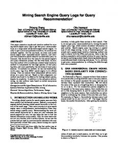
2. Existing Data 2.1. Visible Human Two different sets of 2D images of the thorax have been used to build a spatial processor but both of them derive from the Visible Human Project. It is the creation of a complete data set of 3D anatomically detailed representations of the male and female bodies. [3] The Virtual Soldier and Voxel Man are two data sets derived from the male Visible Human data that have been used for this project. The cadaver has been sectioned at one millimeter intervals in acquiring the transverse images. 2.1.1. Virtual Soldier The Virtual Soldier data is a set of 410 axial labeled images (gif). For this project, only the thorax data set is used and it includes annotations of 437 structures. The axial anatomical images are 2048 pixels by 1350 pixels where each pixel is defined by 16 bits of grey tone. Therefore, each pixel is related to a value that is mapped to a structure name (A text file gives all the mappings).

Figure 1: Sample label image from the Virtual Soldier dataset

2.1.2. Voxel Man The Voxel Man data is a set of 774 axial label images (TIFF) encompassing the abdomen and the thorax. In this series a total of 203 structures were segmented and labeled. [4] The axial anatomical images are 573 pixels by 330 pixels where each pixel is defined by 16 bits of grey tone. It follows the same principle as for the Virtual Soldier data regarding the mapping between the pixel definitions and the structures.

Figure 2: Sample label image from the Voxel Man dataset

5

2.2. Symbolic: Foundational Model of Anatomy (FMA) The Foundational model of Anatomy (FMA) Ontology is an evolving reference ontology for biomedical informatics. It deals with the representation of types of entities and relationships necessary for the symbolic modeling of the phenotypic structure of the human body. A great advantage of the FMA is that it is in a computable form and it is also understandable by humans [1]. Specifically, the FMA explicitly represents a coherent body of declarative knowledge about human anatomy as a domain ontology. The ontological framework can be applied and extended to other species (non-humans) as well. The FMA is considered foundational for two reasons. First, anatomy is fundamental to all biomedical domains. Then, the anatomical entities and relationships encompassed by the FMA generalize to all these domains. The FMA currently contains over 75,000 distinct anatomical types representing structures ranging in size from some macromolecular complexes and cell components to major body parts and the whole organism itself. These types are associated with more than 135,000 terms: preferred names, synonyms or Non-English equivalents. Moreover, they are linked to one another by over 2.1 million iterations of over 200 kinds of relations. This large and complex model is implemented through an approach called disciplined modeling, which consists of a set of declared foundational principles. It is a high level scheme for representing the types of entities and relations in the anatomy domain, scientific definitions and a knowledge modeling environment. This scheme also assures the implementation of the principles and the inheritance of definitional and non-definitional attributes. [5]. The FMA’s high level scheme specifies anatomical entities and the knowledge elements that should be associated with them in a structural context as embodied in the following four-tuple scheme: FMA = (AT, ASA, ATA, Mk) where AT is the Anatomy Taxonomy, which specifies the taxonomic relationships of anatomical entities and assigns them to types according to defining attributes which they share with one another and by which they can be distinguished from one another; the ASA, or Anatomical Structural Abstraction describes a network of spatio-structural relationships between anatomical types represented in the taxonomy; the ATA, or Anatomical Transformation Abstraction describes the timedependent morphological transformations of the concepts represented in the taxonomy during the human life cycle (it includes prenatal development, postnatal growth and aging); and Mk refers to Metaknowledge, which encompasses the principles and sets of rules, according to which the relations and properties are represented in the other three component abstractions of the model. [5] The FMA ontology is implemented in a frame-based authoring environment [6], and is stored in a relational database. The AT types such as Heart, Nerve, and Epithelial cell are formally represented as classes and the relations and properties of these classes such as ‘has_mass’, ‘has_part’ and ‘continuous_with’ as slots. Constraints on allowed values for the slots are called facets. For example, the slot ‘has_part’ for type Heart has facet type Organ part and therefore only organ parts such as the atria and ventricles which are subtypes of Organ part are the allowed slot values. AT types can likewise be instantiated by individual entities or tokens called instances as in my heart, your heart and John’s heart. 6

These four fundamental units, class, instance, slot, and facet are objects called frames. They are “first class objects”, independent from one another but can be readily associated with one another. 2.3. How the Query Engine Has Been Developed The need to acquire and use spatial anatomical information to support various applications in different disciplines of biomedicine is the driving force for this project. Such applications would require the development of a spatial-symbolic query engine which processes spatial information from a data source which in this case are image datasets from CT scans and make them available to users through an interface. The hypothesis is that the spatial knowledge embedded in 2D images can be captured and built up to a 3D level which a spatial query engine can programmatically process into answers to any spatial query. As mentioned in chapter 1.5, the main goal of this project is to build a tool that derives the spatial knowledge from images and combine that with the symbolic structural knowledge already existing in the FMA. The first step is to build the spatial processor which recognizes and understands the most appropriate and explicit definitions of qualitative coordinates as specified by the anatomy expert, and uses the right algorithms and programming languages best suited for this particular project and the graphical user interfaces it requires. Once the spatial query engine is built, the anatomist evaluates the accuracy of the answers provided by the tool and makes suggestions on any improvements or enhancements that will give more accurate spatial information. Then, the project will be focused on developing a faster service in handling and delivering spatial and symbolic structural knowledge.

7

3. Spatial Query Processor Spatial definitions need to be defined before developing a spatial query processor. Depending on the spatial relations being used and the operational needs of the user, the system can be applied in many different ways. In this study, an anatomist defined the spatial relations that are appropriate and prevalent in the domain of anatomy. Once the spatial definitions have been clearly defined and validated by an anatomist, the next step requires choosing the most appropriate tools (programming languages, algorithms) to implement the system. After the spatial query processor is built, an application (applet) is then developed to provide for an intuitive method that would enable a user to easily query the system for information about spatial relations between anatomical structures. 3.1. Definitions of Spatial Relations Defining the spatial relations is not easy as there are no existing formal definitions for them. An anatomist was solicited to provide operational definitions for the kind of spatial knowledge that is commonly used in the discourse of anatomy and can best provide suitable answers to spatial questions. Because the symbolic definitions of spatial relations are not explicitly described, the initial attempt to implement spatial description for the graphical model was equally inadequate, resulting into conflicting and sometimes wrong results. Therefore new definitions have been considered in order to approximate as closely as possible the spatial relations that anatomists and clinicians are familiar with and which they use for their respective domains. The definition of the anterior relation is the first to be refined and once determined satisfactory, its definition has been adapted to describe the other relations: posterior, rightlateral, left-lateral, inferior and superior. 3.1.1. Anterior: Simple Definition The first definition that was studied is quite simple and does not require any computations for the shapes involved in the anterior area. The method simply detected whether a structure, its whole or its part, is within the spatially defined area.

Figure 3: Anterior relation, simple definition

The anterior spatial relation is defined as follows: ‘A structure is considered as anterior if at least one of its voxels is within the grey volume or area as defined in figure 3’. The results obtained with this definition gave both satisfactory and unsatisfactory results. In fact, some structures were considered 8

anterior whereas they should not but some other structures were correctly considered anterior. A structure A may very well be lateral to the target structure B but because a single voxel of A happens to be included in the anterior area defined for B, A becomes imprecisely implied as being anterior to B. Adjustments to the definitions had to be made to reflect a more accurate and acceptable spatial relationship. (See chapter 4) 3.1.2. Anterior: 90 Degree Angle and Ratio This definition involves the computation of the number of voxels of each shape contained partially or not in the anterior volume. The first step is to establish the range or scope of the volume or “slice” anterior to a specific structure and then determine what other structrures fall within that anterior volume or “slice”, as shown in figure 4. Then, for each shape involved in this anterior slice with at least one voxel, the number of voxels involved, out of the total number of voxels of the shape, is computed. As a result, a list with all the shapes involved associated to their percentage of involvement is therefore obtained. The last step is to define a threshold value, i.e. all the structures whose volume percentage based on pixel count cross the threshold value are considered anterior. If the percentage is below the threshold value, then the structure is eliminated from the list. An arbitrary default value has been defined by an anatomist at 40% as a test to the efficacy of the method. Ultimately, it will be the user who will determine the threshold value which is best suited for the user’s particular application.

Figure 4: Anterior definition, 90 degree angle and ratio

In figure 4, the analyzed shape is simple, i.e. the center of mass for each slice (z axis) has the same coordinates x and y. The 3D model is built from 2D images and instead of computing the general center of mass of the whole shape, the intermediary centers of mass from each slice are used to define the anterior volume. As a result, the anterior volume is specific to each anatomical structure since the centers of mass probably have different coordinates for each slice. 9

3.1.3. Posterior, Left-Lateral, Right-Lateral: 90 Degree Angle and Ratio As depicted in figure 5, other spatial relations, i.e. posterior, left-lateral and right-lateral, follow the same definitional principle used for the anterior relation. The volume (e.g. posterior) is defined the same way, which also necessitates the computation of the coordinates of the centers of mass. Only the direction of the volume differs depending on the spatial relation.

Figure 5: Posterior, left-lateral, right-lateral (90 degree angle and ratio)

3.1.4. Superior, Inferior Similarly, the superior spatial relation involves the computation of a ratio: the number of voxels contained in the superior volume as defined in figure 6 out of the total number of voxels of the considered anatomical structure. As such the anatomical structure is considered as being superior depending on the computed ratio and the threshold value set by the user.

Figure 6: Superior relation

Note that the superior volume is defined by considering the space above the plane tangent to the highest voxel of the anatomical structure. The inferior relation follows the same principle. 3.1.5. Surrounding Structures When dealing with the first results of the spatial query processor, it appeared that surrounding structures registered as anterior, posterior, right-lateral or left-lateral to the surrounded structure. The 10

filter consists of reading pixels in each direction (anterior, posterior, right-lateral and left-lateral) for a few slices of the structure where the surrounding structure is also labeled. If it occurs that the structure has some labeled pixels in all four directions for at least one slice, it becomes considered as a surrounding structure and therefore, it is not considered anterior. The reading of the pixels is described in figure 7. For a few slices of the structure, four virtual lines are drawn from the center of mass of the structure for the slice, and the pixels along the lines are read. If the structure first considered anterior has also labeled pixels in each direction, it becomes considered as a surrounding structure. The slices are randomly chosen among all the slices where the main structure and the structure first considered anterior have both labeled pixels.

Figure 7: Detecting surrounding structures

3.2. Processing of the 2D Images Processing the images to build a 3D model is the main part of the project and involves choosing the appropriate tools primed for quick development and have the required features to give satisfactory results right away. 3.2.1. Different Possibilities to Build a 3D Model As part of the project, it is necessary to check the existing tools that could help to build the image processor. 3.2.1.1. Mind Seer A tool for multi-modality neuroimaging data called MindSeer was developed by the Structural Informatics Group. It aims at visualizing 3D surfaces and the demo version enables the users to visualize a 3D representation of the brain [7]. A great advantage of using MindSeer is that new features would be added to an existing tool built by the Structural Informatics Group. Moreover, the code is written in Java which is a key-point since most of the projects led by the team use Java as a primary programming language. Another great advantage is the fact that the visualization of the answers would be possible. For example, an answer to the question ‘What is anterior to the heart?’ could be a direct visualization of all the structures involved in addition to the list of names of those structures. 11

However, the code of MindSeer tool is not fully documented and no tutorial is available to add a plugin that would enable a software developer to add new features easily. For this major reason and given the time frame, MindSeer was not chosen to develop the spatial processor. In figure 8, a screen shot shows the 3D visualization of the brain with MindSeer.

Figure 8: Screen shot, Mind Seer, Structural Informatics Group

3.2.1.2. 3D Slicer 3D slicer is a multi-platform, open-source software for visualization and image computing [8]. Its major advantage over MindSeer is that it is widely used by a large community. That means that it would be easier to get answers regarding the code or the structure of the program thanks to forums. In addition, the documentation is quite abundant, which would make it easy to learn about the software program. It would require some time to understand the existing code and add new features to build a spatial processor. Given the time frame, 3D slicer was not chosen as well to build the spatial processor. 3.2.1.3. Geometric Tools Geometric tools is a C++ package that enables a developer to perform complex mathematic operations: image analysis, numerical methods. [9] This package offers the possibility to compute easily and with efficiency the intersection of shapes, e.g. rectangles. This package also allows the distance between two different shapes to be computed with ease. The versatility of the package and the fact that a lot of geometric operations can be performed makes it a good candidate. However, most of the projects within the Structural Informatics Group are developed in Java. Therefore, developing a project in C++ would not be likely to be followed-up. Moreover, all the features offered by the Geometric Tools plug-in would probably not be used for the basic features like the detection of anterior anatomical structures for example. 3.2.1.4. Java 3D Java 2D/3D is a Java library that enables a developer to provide a three dimensional content to users. [10] [11] The development of a spatial query processor requires the possibility to develop a 3D model based on 2D images that contain shapes with very specific outlines. However, java 3D is designed to provide a high-level view of 3D graphics but not necessarily for 3D mathematic operations and computations. [11] Creating a scene generator would be an interesting feature but it is not the primary 12

goal of the project, which is the development of a query processor. As a consequence, the plug-in will not be used for the project. Furthermore, a project at the Structural Informatics Group named Biolucida and led by Wayne Warren, PhD student, aims at developing a scene generator of anatomical structures of the body. [12] Eventually, a plug-in could be developed so that the spatial query processor can be used with the scene generator and provide a 3D visualization of the answers such as all the anatomical structures anterior to the heart for example. 3.2.1.5. Java from Scratch After a careful review of the different existing tools that could be used for the project, it was decided to start from scratch with Java. Only the algorithms to process the images need to be created and the mathematical operations are not so complex that an external library should be used. The algorithms imply defining the anterior (or posterior, etc.) volume to a structure and calculate the number of voxels of all the shapes involved. Java is a programming language that the team at the Structural Informatics Group uses mostly for their projects, so it becomes important to use a programming language that makes it possible for the team to follow-up and pick-up the project. 3.2.2. Architecture Java is the programming language used for the spatial query processor that will process the images and build a 3D model from which to derive the spatial anatomical knowledge required to answer questions related to spatial relationships between anatomical structures. As indicated above, the answers will take into account the definitions of spatial relations proposed by the anatomist. The program consists of different packages: the ‘data’ package and the ‘algorithm’ package. The ‘data’ package deals with the reading of files containing the mappings between the structure numbers and the structure names for the datasets: Virtual Soldier and VoxelMan. This package also deals with the connection to a database used to save intermediary results. The ‘Algorithm’ package deals with the different algorithms used for every spatial relation: anterior, posterior, right-lateral, left-lateral, superior, inferior. It also deals with the loading of the images. There are two main classes (each class is related to a dataset: Virtual Soldier and Voxel Man) that load the images, i.e. they store the position of all the shapes so that the processor can answer questions about spatial relations between anatomical structures. Once the images are loaded, a developer can use the other classes about spatial relations to find out the anterior structures to a specific structure for example. Finally, the mapping is done thanks to the ‘data’ package to relate the structure numbers to their name.

13

Figure 9: Functioning of the spatial query processor

In figure 9, the functioning of the spatial query processor is described with the features it offers. The program needs an input, which is the combination of the structure to be analyzed and the spatial relations that need to be checked associated with a threshold value. Then, the program loads all the images by reading them and performs the adequate calculations in order to answer the question. Finally, the program outputs a list of structures as an answer. It is actually possible to input any anatomical structure labeled in the dataset (Virtual Soldier or Voxel Man) and any spatial relation. 3.2.3. Algorithms 3.2.3.1. Storage of Shape Descriptions The choice of the algorithms is crucial in terms of the efficiency required in providing the spatial query processor the ability to deliver quick answers. The first issue to be addressed is how the location of the shapes is stored and how the stored data is handled to answer a spatial query. For each image, every pixel is read and since the location of the pixel is known (image number and position on the image), it is possible to determine where a labeled anatomical structure is located exactly with no approximation. Instead of storing a list of all the 3D points where a structure is present, which would obviously be wasteful, a map is used to store the 2D outlines. It is crucial to represent accurately the data and not to make any approximation to build a 3D model. Therefore, it is difficult to avoid the storage of a large amount of data. Each structure is related to a map that has the following structure: Key: ‘z’ (related to the image number); Value: another map. For each map related to z, the key is ‘y’ and the value is a point. The way the map is used makes it easy to retrieve a point that belongs to a structure when z and y are known. Of course, if only x and y are known, it takes more time to get an answer. At this stage of the project, what matters is to get a first query processor that generates answers to spatial queries. 14

The algorithm used for the first version of the spatial query processor has been conceived so that it can be used and can provide results that can be analyzed by an anatomist who can then refine or update the definitions of spatial relations when needed. At this stage, efficiency is not a key-point. The maps related to the anatomical structures contain some points that enable the system to locate accurately the shapes. For each slice, the outline is stored but in fact some points have been discarded. An example is provided to explain how some points have been discarded and therefore, how some memory space has been saved.

Figure 10: Example of an image with labeled pixels

In figure 10, some labeled pixels are displayed and are related to the same anatomical structure. The issue here is to translate what is read from the images and store in some way the location of the shape. A simple algorithm would result in storing all the points (pixels) that define the outline as shown in figure 11: each pixel (x,y) that is not surrounded by four pixels at locations (x+1,y), (x,y+1), (x,y-1) and (x-1,y) will be stored.

Y For y from 0 to (width-1), x from 0 to (height-1) If not (pixelDown, pixelUp, pixelLeft and pixelRight belong to the shape) Save point;

X

Figure 11: Storing the outline of a shape on a 2D image

15

A simple way would consist of storing all the points of the outline. Even if there is no approximation, it requires a lot of memory to store all the outlines of the shapes for each slice. Additionally, a mechanism should be found to retrieve the actual shape of the structure based on the saved points. In order to save some memory space and even if the goal is to develop a first version of a spatial query processor without dealing with the efficiency issue, another mechanism has been used to store the location of the shape. In figure 12, the algorithm and a scheme illustrate how the mechanism works and how it can save some memory space.

Y

X

For y from 0 to (width-1), x from 0 to (height-1): if(point(x,y) is not at the top of the image AND point(x,y) is not at the bottom of the image) {//3 possibilities if (pixelDown and pixelUp do not belong to the shape) // the point is isolated, we add it to the list save point (x,y); else if (pixelUp belongs to the shape but not pixelDown) // Lower bound save point(x,y) as a lower bound; else if (pixelDown belongs to the shape but not pixelUp) //Upper Bound save point(x,y) as an upper bound; } else if (point(x,y) is at the bottom of the image) if (pixelUp belongs to the shape) save point(x,y) as a lower bound; else save point (x,y); } else if (point(x,y) is at the top of the image) if (pixelDown belongs to the shape) save point(x,y) as an upper bound; else save point (x,y);

Figure 12: Storing the outline with lower and upper bounds

As explained in figure 12, each pixel is read and there are three possibilities: If the point is neither at the bottom nor at the top of the image (which means it has at least one pixel above and at least one pixel below): o If the pixel above and the pixel below do not belong to the same structure as the current pixel, it means it is considered as an isolated pixel and it is stored. o If the pixel above belongs to the same structure but not the pixel below, the pixel is stored as a lower bound. o If the pixel below belongs to the same structure but not the pixel above, the pixel is stored as an upper bound. If the pixel is at the bottom of the image: either the pixel above belongs to the structure and in that case, it is stored as a lower bound, or the pixel is stored as an isolated point. 16

If the pixel is at the top of the image: either the pixel below belongs to the structure and in that case, it is stored as an upper bound, or the pixel is stored as an isolated point. This algorithm can be improved in different ways. First, it only deals with lower and upper bounds in one dimension with the x axis. The same principle could be used in two dimensions or even in three dimensions. Other ways of representing the data may be used as well. An important part as well is how the location of an object can be retrieved. For the first version of the spatial query processor, maps are used and it is enough to retrieve the location of an object. Once again, efficiency is not the primary goal for now and therefore, subsequent work must be done in order to conceive an efficient spatial query processor that can be queried fast. 3.2.3.2. General Mechanism: Handling a Query 3.2.3.2.1. Simple Mechanism To begin with, a simple mechanism was used in order to achieve a first spatial query processor so that an anatomist can analyze the results and decide whether the results are satisfactory or not. In the latter case, the definitions would need to be redefined. Given a structure, this first algorithm implies the definition of the anterior part (or any other spatial part), which is a slice defined by the center of mass of each image in which the structure contains some pixels. Beforehand, the spatial location of all the shapes has been stored. When handling a query such as ‘What is anterior to the heart?’, the query processor simply checks every pixel in the anterior part (or any other spatial part depending on the query such as the posterior part for example) and store the number of pixels for each shape involved. Since the total number of pixels of the shapes has been stored beforehand as well, it is easy to compute the ratio and determine the answers to the queries thanks to the threshold value defined by the user. The algorithm that consists of checking every pixel is quite simple but time-consuming to determine the answer to the question. It is summed up in figure 13 with the example ‘What is anterior to the left lung?’ but the principle remains the same for all the spatial questions.

17

Figure 13: Simple algorithm, 'What is anterior to the left lung?'

3.2.3.2.2. Mechanism more Complex: Octrees The first algorithm used for the spatial query processor helps to get results for spatial questions but it has been proven not to be very fast. Therefore, the next step is the building of a faster query processor that would provide answers to spatial questions with the same accuracy but more quickly. In order to achieve the development of such a processor, the algorithm used to determine the answers to the questions needs to be changed or improved. The issue is to pre-compute as much as possible some results so that when a query is being handled, the system does not have to perform a lot of computations. The point is to partition the space (i.e. the thorax in the study) and use a tree data structure that would retrieve quickly where an anatomical structure is located. The octrees are commonly used for spatial indexing; the three dimensional space is recursively subdivided into up to eight octants: each internal node has up to eight nodes. How have the octrees been used in order to build the spatial query processor? Consider the example in figure 14. In the example, each node has four children but for the actual processor, each node has eight children.

18

Figure 14: Octrees, 2D example, level 0

Assume the space is a square and there is a circle in the space. What structures are anterior to the circle? First, the anterior part (which is a 2D slice) must be defined, and then the number of pixels of the anatomical structures contained in this area must be computed to determine the answer. The octrees help to compute the number of pixels because of pre-computations. The first step for applying the octree algorithm is to read every pixel contained in the space. In the example, the first step is to read all the pixels contained in the square. For the actual space from the data used to build the processor, the first step is to read all the pixels from the images. As a result, the number of pixels for all the shapes is known for the entire space. The entire space is root 0 in the tree structure. The next step is to divide the space into four parts as shown in figure 15.

Figure 15: Octrees, 2D example, level 1

In the example, node 0 has four children: 00, 01, 02 and 03. The same task is done for each node, which means for each node the number of voxels of the shapes is computed. As a result, it is possible to determine if an anatomical structure is contained in a node and how many voxels are involved. 19

Figure 16: Octrees, 2D example, level 2

In figure 16, each node from level 1 (00, 01, 02, 03) has four children. The same principle applies and the number of pixels of all the shapes is computed for each node. Therefore, the space has been partitioned into nodes and subnodes, and this helps to determine the anterior structures faster. In comparison to the simple algorithm, the octrees use pre-computations. Consider figure 17. Which structures are anterior to the circle? The simple algorithm would check every pixel in the anterior part in order to determine the number of pixels of the shapes contained partially or not in the anterior part. The octree algorithm will first check all the complete nodes involved in the anterior part. Performing such an operation will save computations because finding complete nodes means that the number of voxels involved in the node is known for each shape. However, if incomplete nodes are found, every voxel from the incomplete nodes must be checked to determine accurately the number of voxels of the shapes involved.

20

Step 1: complete nodes involved Step 2: pixels that are not in complete nodes

Figure 17: Octrees, 2D example, principle

Depending on the depth of the tree structure, the number of voxels contained in a node varies. For the Virtual Soldier data set, if depth is equal to four: there are 4,096 leaves and each leaf contains 276,750 voxels. Similarly, if depth is equal to five, there are 32,768 leaves and each leaf contains 32,593 voxels. Figure 18 presents the general principle for the octree algorithm with the example ‘What is anterior to the left lung?’. The differences with the simple algorithm used previously are emphasized: pre-computations of the number of voxels of each shape in the nodes and the use of those precomputations when handling a query.

21

Figure 18: Octree algorithm, 'What is anterior to the left lung?'

3.3. Application The spatial query processor built is highly capable of handling any spatial query but delivery of response is still slow. The process involved in producing the answers is currently quite time-consuming, often requiring several minutes, and for application users, this is unacceptable. Therefore the focus is to improve efficiency either by developing a more efficient spatial query processor or use databases where all the results would be pre-computed. Given the time frame and the goal of the project, it has been decided to work on the databases rather than spend more time in developing a more efficient spatial query processor. 3.3.1. Use of Databases In order to develop an interface that is able to provide quick answers to spatial questions, the storage of pre-computed results has been used. In fact, all the possible questions have been handled and their answers stored in a database. That means that for each anatomical structure, all the spatial relations (anterior, posterior, right-lateral, left-lateral, superior, inferior) have been analyzed and the percentage related was stored. As a result, when handling a query, the database is queried with a given percentage, and the answer is retrieved from the database. The scheme of a table is rather simple: Structure_ID, RelatedStruture_ID, Percentage. There is one table for each spatial relation (i.e. anterior, posterior, left-lateral, right-lateral, inferior, superior). The primary key is the combination of the two columns: Structure_ID and RelatedStruture_ID. RelatedStruture_ID is the id of the structure connected to the structure whose id is Structure_ID considering the spatial relation that the table is defined for.

22

Only the thorax has been analyzed for this study. The Virtual Soldier data contains 437 labeled structures and the Voxel Man data set contains 203 labeled structures. When dealing with an SQL database where each table is related to a spatial relation, the number of rows can be big depending on the spatial relation. The anterior and posterior tables contain about 25,000 rows; the right-lateral and left-lateral tables contain about 35,000 rows; the superior and inferior tables contain about 80,000 rows. If the whole body was labeled with FMA terms (several thousands anatomical structures), the table would contain much more rows and therefore, it would be difficult to handle queries. The need to develop a spatial query processor that handles queries at run-time would be necessary. Such a project would require more detailed research on how to retrieve spatial data, use pre-computations and compute efficiently. 3.3.2. Features A client-server application and an applet were developed. Both have exactly the same features, only the way they are deployed is different. Both applications use the same interface that enables a user to query the database that has been built beforehand. A user can select the anatomical structure and the percentage for each spatial relation. Figure 19 shows a screen shot of the interface. When selecting a structure, the tool provides a list of all the anatomical structures that are related to the selected structure considering the different spatial relations and the input percentage. This application is mainly an interface to query a database so that an anatomist can check the results and make new suggestions for improved definitions or additional perspectives. Moreover, any user may also use the service to get to learn about spatial relations.

Figure 19: Screen shot, interface to query the pre-built database

23

4. Web Service Related to the FMA and the Spatial Database The spatial query processor was built and all the answers it can provide were stored in a database. As a consequence, it is now easy to query the database to retrieve answers about spatial queries. The FMA ontology has already been built as well in a different database. The next step for the project is to create a higher level system that can handle FMA and spatial queries. 4.1. FMA Query Engine The FMA is accessible through a web service that uses Jena and Sparql. In fact, the FMA is stored as an RDF graph. RDF is a labeled data graph format for representing information in the web. [13] RDF graphs are related to distributed knowledge and follow some principles. [14] First of all, files on the web need to be able to express information flexibly. Graphs are commonly used with triples: Subject, Property and Object. Then, the files need to be related to each other. Finally, the information should be consistent, i.e. two files dealing with the same entities with different names should be able to be mixed together. The Jena project is a semantic web framework for Java, and is used to deal with the FMA ontology since Jena provides persistent storage of RDF data in relational databases. [15] In order to query an RDF graph with Jena, some Java code must be written and Sparql, a query language for RDF, may be used to query the graph. [13] The structure of the RDF graph for the FMA ontology is quite complex. As a result, some help was required to understand exactly what properties were needed to query the FMA and also how they should be queried (structure of the query: subject-Property-Object). 4.2. Spatial Database So as to be consistent with the FMA ontology, a spatial database was built as an RDF graph, making it possible to query both databases (FMA and spatial) within a single Sparql query. The RDF graph scheme designed for the spatial database uses bags from the RDF typed node elements. As shown in figure 20, each entity (i.e. anatomical structure) is related to an URI. In the example, the URI is structures:119. The prefix ‘structures’ is a name for a longer URI which can be anything; for instance, it can be http://uw.structureslist.com/. It is a way to uniquely identify the anatomical structures. An entity has obviously a name and this property is symbolized by the triple: object (entity)-Property (‘hasName’)Object (String). RDF graphs are designed with triples. Moreover, each entity has a list of anterior structures. It is represented with the triple: Object (entity)-Property (‘listAnteriorStructures’)-Object (Bag of pairs entity-percentage). The percentage describes how anterior a structure is. Every other spatial relation (posterior, right-lateral, left-lateral, superior, inferior) is represented the same way with bags.

24

Figure 20: RDF graph scheme designed for the spatial database (only some of the spatial relations are represented)

4.3. Architecture The web service has been specifically designed to access both data sources (FMA and spatial knowledge base) by using the same query language. Sparql allows querying two data sources within only one query but requires the path to the RDF graphs (file, e.g. XML format). Since the RDF graph for the FMA ontology contains a huge amount of information, it is time-consuming to retrieve data from such a file. Therefore, the work of Marianne Shaw, PhD student at the University of Washington, was used in order to query with Sparql two relational databases that represent RDF graph thanks to the Jena framework. [16] The terms used by Virtual Soldier or Voxel Man differ from the terms used in the FMA. However, an anatomist built the mapping between the FMA and the data sources, making it possible to query both data sources.

25

Figure 21: Architecture of the FMA-spatial web service

In figure 21, a scheme of the architecture of the whole system is represented. An interface enables users to define the question they would like to get an answer to. Then, the query engine deals with the query and accesses both data sources in order to get an answer to the query. 4.3.1. Web Query Interface 4.3.1.1. Principle The web query interface deals with the potential queries users may request. Queries are related to the FMA and spatial relations. Given the time frame of the project, only the ‘is_Organ’ relation has been implemented. This relation means ‘is the anatomical structure an organ?’. Since the system can directly access the FMA ontology and all the parameters have been set up, it would be easy to add new properties for anatomical structures related to the FMA. Regarding spatial relations, all the templates for different questions have been implemented. The structure ‘Subject-Relation-Object’ has been chosen because it enables users to answer lots of questions regarding the FMA and spatial relations.

26

Figure 22:'Subject-Relation-Object' structure

The web service deals with anatomical structures; therefore, the subject and the object are either a set of anatomical structures or a single anatomical structure. In figure 22, a scheme of the ‘SubjectRelation-Object’ structure is represented. The ‘relation’ in the ‘Subject-Relation-Object’ structure can have different values: unknown, spatial (by specifying a spatial relation, i.e. anterior, posterior, rightlateral, left-lateral, superior, inferior), logic (union or intersection of sets and/or single anatomical structures), FMA (only the ‘is_Organ’ relation has been implemented so far). The goal is to answer a simple question whose structure is ‘Subject-Relation-Object’. For example, ‘What is anterior to the heart?’ is such a question that can be answered with only one query: the subject is unknown, the relation is the anterior relation and the object is the heart. If a question is more complex, it must be divided into simple sub-questions and use intermediate results (sets of anatomical structures). There is an example in figure 23. The complex question requires using intermediate queries whose results are saved (intermediate sets) so that next questions can be handled by using those results.

27

What is the spatial relation between the left seventh rib and the organs that are postero(16%)-right-lateral(29%) to the lower lobe of left lung? Structure of each question: Subject Relation Object Set 1: anatomical structures postero-right-lateral to the lower lobe of left lung Unknown Postero-right-lateral Lower lobe of left lung Set 2: organs from Set 1 Set 1 Organ Unknown Text (answer): Set 2 Left seventh rib Set 2 Unknown Left seventh rib Figure 23: 'Subject-Relation-Object' example, complex question

4.3.1.2. Implementation The web query interface was implemented with OpenLazslo, which is an open source platform for the development of rich Internet applications. This programming language was used for its features that make the interface easy to handle.

Figure 24: Screen shot of the web query interface

In Figure 24, an example of the use of the web query interface is shown. The structure ‘SubjectRelation-Object’ is noticeable. The example shows the definition of the query ‘What is anterior to the lower lobe of left lung (40%)?’. Then, the user would need to click on the ‘Query’ button to get an 28

answer to the query. The result is shown in figure 25. The list of anatomical structures is sorted out in descendant order (percentage).

Figure 25: Screen shot, result of the query 'What is anterior to the left lung (40%)?'

4.3.1.3. Query Engine and Databases The query engine is developed in Java and uses the Jena tool to access and query relational databases that represent RDF graphs. Sparql is the RDF query language used for the project. In figure 26, a sample query shows how similar Sparql is similar to SQL about the query structure. What differs mostly is the ‘where’ clause: triples mix variable names and properties related to the queried RDF graph(s). When the FMA ontology is queried, only the FMA relation ‘is_Organ’ is involved for the web service. However, it implies to determine whether or not a structure is an instance of a class that is a subclass of the ‘Organ’ class. In order to achieve this, the transitivity property is necessary. Since it is not implemented in Sparql, Gleen was utilized for the web service so that the transitivity property can be used. Gleen is a plug-in for Sparql developed by a software developer at the University of Washington and enables developers to use regular paths when dealing with Sparql. [17]

29

L1: PREFIX relations: L2: PREFIX rdfs: L3: PREFIX fma: " L4: PREFIX gleen: L5: SELECT ?organ ?anterior_structure_name L6: FROM L7: FROM NAMED L8: WHERE { L9: ?organ relations:hasName ‘Abdominal part of esophagus' . L10: ?organ relations:listAnteriorStructures ?list . L11: ?list rdfs:member ?node. L12: ?node relations:relatedStructure ?anterior_structure. L13: ?anterior_structure relations:hasName ?anterior_structure_name . L14: ?node relations:percentage ?per . L15: FILTER ( ?per >=10 ) L16: GRAPH{ Gleen L17: ?anterior_structure gleen:OnPath (\"[rdfs:subClassOf]*\" fma:Organ) . L18: }. L19: } Figure 26: Sample Sparql query to two data sources

In figure 26, the query engine answers the question ‘What organs are anterior to the abdominal part of the esophagus (10%)?’. It provides a list of all the organs anterior to the abdominal part of the esophagus with a ratio (involvement in the anterior volume) greater to 10%, i.e. an organ whose the number of voxels involved in the anterior volume is greater than10%. The query begins on line 1 with the prefix used within the query and aims to read more easily a query. They symbolize URIs for properties and entities. In the ‘Select’ clause, variable names are noticeable because they begin with a question mark. Then, the ‘from’ clauses define the location of the sources (RDF graphs). Line 9, in the ‘where’ clause, aims at getting the entity (variable name: ?organ) whose property ‘relations:hasName’ (URI for the property ‘hasName’) is ‘Abdominal part of esophagus’. Then, line 10 gets the list of the anterior structures. Line 11 deals with every node included in the list of anterior structures. Line 12 gets the actual anterior structure included in the node and the next line gets the name of this anatomical structure. Line 14 gets the percentage relation to the anterior structure. In the ‘where’ clause, it is possible to use a filter in order to select a part of all the answers already retrieved; here, only the anatomical structures with more than 10% of involvement in the anterior part are kept as a result. Finally, the sub-clause ‘Graph’ is used to query another source, i.e. the FMA ontology, and Gleen is utilized to determine whether a structure is an organ.

30

5. Evaluation The web service was evaluated and the results of queries were analyzed by an anatomist. In fact, the anatomist was the guide and the one who decided whether or not the results were accurate enough. He also refined or adjusted the definitions of spatial relations accordingly. Moreover, the time response of the query processor was optimized. 5.1. Accuracy Accuracy is a key point in this study and it is important that answers to questions dealing with spatial relations correspond to the anatomist’s point of view. In the initial attempt, the definition for anterior relation was found inadequate and insufficient to provide accurate results. Therefore adjustments were made in the definition of the anterior relation to improve accuracy. The simple definition of the anterior relation takes into account some of the shapes that the more complex definition does not, and vice versa as the two examples demonstrate below. Additionally, implementing the ratio helps to define ‘how’ a structure is considered anterior to another structure.

Figure 27: Anterior relation, simple definition, 90 degree and ratio

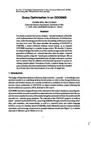
As proof of concept, consider the Virtual Soldier data set and the example: What is anterior to the left sixth costal cartilage? On the left hand side of figure 27, a scheme reminds what the simple definition of the anterior relation is. Regarding this definition, the answer to the question is: subcutaneous tissue of trunk: surrounding skin of trunk: surrounding sixth external intercostal muscle sixth internal intercostal muscle left sixth rib left seventh costal cartilage fifth internal intercostal muscle pectoralis major muscle body of sternum: wrong

31

On the right hand side of picture 27, a scheme reminds what the more complex definition of the anterior relation is (90 degree angle and ratio). Regarding this definition, the answer to the question is: left seventh costal cartilage (1.65%) pectoralis major muscle (0.06%) fifth internal intercostal muscle (0.4%) sixth internal intercostal muscle (0.0%) body of sternum (0.0%) Note that for the second definition, a filter detecting the surrounding structures was applied and therefore, no surrounding structure appears in the results. Both answers have similarities but the answer for the first definition consists of more anatomical structures. Some of them are not correct because they surround the left sixth costal cartilage, i.e. the subcutaneous tissue of trunk and the skin of trunk. The body of sternum is not considered anterior and therefore, it should not be given as an anterior anatomical structure to the left sixth costal cartilage. The definition that implies the computation of the ratio is more accurate and gives more information. In the example, the spatial query processor gives fewer structures for the definition of the anterior relation that implies a 90-degree-angle slice. In figure 28, a transverse slice where the left sixth cartilage is displayed shows that the configuration makes it possible to obtain more structures contained in the anterior area when dealing with the simple definition of the anterior relation. In fact, the sixth external intercostal muscle and the left sixth rib do not have a single voxel in the anterior volume defined with the complex definition of the anterior relation.

Figure 28: Transverse slice, left sixth costal cartilage

However, this analysis may be different for some other structures. Consider the left conus artery. The simple definition of the anterior relation gives fewer structures than the more complex definition. It is explained by the fact that some structures are far away from the analyzed structure, and they are 32

located on the sides, therefore the anterior volume for the simple definition does not contain them whereas the anterior volume from the more complex definition does. 5.2. Data Problem Before using the Voxel Man data, the Virtual Soldier data set was used for the study and the building of the spatial query processor. After the first definition of spatial relations was given by an anatomist, the spatial query processor provided unexpected answers. First of all, the surrounding structures were taken into account. Therefore, some structures (typically the skin of trunk) were considered anterior where in fact only a segment of the skin is anterior but with reference to the entire skin, the association is inaccurate. Then, it appeared that the dataset consisted of a few wrongly labeled pixels for some of the pictures. 5.2.1. Wrongly Labeled Pixels

Figure 29: Sample image, Virtual Soldier, wrongly labeled pixels

In Figure 29, some pixels in the right-hand-side corner of the image are labeled: it is an error in the dataset that occurs on most of the images and it must be handled in order to get more accurate answers. The spatial query processor simply discards the wrongly labeled pixels when processing the images. For each image, a rectangle is virtually defined and all the pixels contained in this rectangle are discarded. The rectangle is defined depending on the location of the pixels that must be discarded and it is dynamically handled when processing the images. Another possibility could be a modification of the images. However, the data set consists of 410 images and it would be time-consuming to perform this task. 5.2.2. Dataset not Accurate Enough Some anatomical structures are located on the right and left sides of the body, e.g. the lungs. Therefore, there should be a distinction between the left and right lungs in order to handle accurately spatial relations. Those two anatomical structures are both contained in the data set. However, a distinction should also be made for other structures like the eighth internal intercostal muscle, but the data set does not distinguish the eighth internal intercostal muscle between the left eighth internal intercostal muscle and the right eighth internal intercostal muscle.

33

This distinction is necessary because the spatial associations between the right and the left structures are different and therefore their own attributes must be encoded in the spatial knowledge base. So queries specific to a particular side can be readily accessed.

Figure 30: The distinction between the left and right structures matters when dealing with the anterior relation

Figure 30 depicts a scheme where in the anterior volume of a structure the left and the right versions of the same structure (e.g. right third rib and left third rib) are not marked separately. Given the definition of the anterior part (90-degree slice), finding the anatomical structures anterior to such a structure is not accurate. Improving the accuracy of the labels, i.e. making a distinction between the right and the left structures when necessary, requires the work of an anatomist who would need to analyze all the structures and images where they are involved. This task was not performed on the available images used for this work. 5.2.3. Duplicate Data Another issue has been discovered when analyzing the answers to spatial questions from the first definition (simple definition), and deals with annotation of the same data with different terms. This is true particularly in cases where a part of a structure is labeled at one level as the proper part and at another level as the entire structure. For example in some cross sections the pixels are labeled as the left and right atriums and the left and right ventricles but in a few other sections the corresponding pixels are labeled as the heart itself. This inconsistency therefore can lead to confusion for the program and may result in retrieval of inaccurate answers. Once again, only an anatomist can provide the correct and appropriate labeling, but this work has not been performed due to time constraint. 5.3. Response Time To achieve a quicker response time, the octree algorithm was applied with the intent of deceasing the requisite computations involved in the process. This is true when the anterior volume (slice) consists of a big amount of voxels so that some complete nodes are included. Otherwise, the method may result in a slower service because the algorithm checks first the included nodes and then 34

the voxels that are not included in the nodes must be eventually checked. Therefore, if there are only a few complete nodes included in the anterior volume or no complete node, the other voxels must be checked one by one. Here are two examples to illustrate this point when answering the question ‘‘What is anterior to …?’: Third anterior intercostal vein: 6,532 ms (octree algorithm); 3,171ms (simple method). Left sixth costal cartilage: 6,547ms (octree algorithm); 2,671ms (simple method). However, the octree algorithm is faster for the structures whose size is important because they avoid the reading of the pixels contained in the complete node included in the anterior volume. Here is another situation where two examples answer the question ‘‘What is anterior to …?’: Anterior basal branch of left pulmonary: 5,485ms (octree algorithm) ; 32,093ms (simple method) Right first rib: 8,046ms (octree algorithm); 20,704ms (simple method) Building a web service with quick response time is obviously important and desirable, and therefore it has been decided to first compile all the answers and then store them in a database. This was the most reasonable option to pursue given the limited time frame allotted for this study and where a web service needs to be developed.

35

6. Conclusion The development of a spatial-symbolic query processor in this study serves as proof of concept from which more complex methods or systems for querying more sophisticated spatial relations can be developed not only for the biomedical field but also for the non-biomedical domains. The study started with the proposed definitions of spatial relations by an anatomist and which were iteratively updated to provide more accuracy in the representation. The goal was to develop a spatial query processor that deals with spatial relations between anatomical structures but also uses symbolic knowledge combined with spatial information generated by the spatial query processor. The processing of 2-D images is the key-point in first developing a spatial knowledge base which then serves as the primary spatial information resource for the query processor. The hypothesis was therefore correct, i.e. using 2D images to compute qualitative spatial coordinates and determine relations between anatomical structures. Moreover, the spatial query processor was proved to handle any data set since two different data sets (Virtual Soldier and Voxel Man) were used for the study. It provides spatial knowledge about anatomical structures based on commonly used qualitative coordinates defined and used by anatomists. The spatial query processor was able to handle spatial queries such as 'What is anterior to the left lung?'. Also, a higher-level system was built as a web-service and was ready to handle queries dealing with both spatial and symbolic knowledge, which was the goal of this study. Since the FMA ontology was represented as an RDF graph, it was necessary to represent the spatial database as an RDF graph in order to acquire a homogeneous system. Finally, two RDF graphs were used as sources and were queried by using the same query language through a web interface. The web service can handle queries such as 'What organs are anterior to the left lung?'. Diverse tools and libraries have been used in the development of the query processor and the subsequent deployment of a web service: OpenLazslo, Java, Tomcat, Gleen, Sparql. During the study, new innovative ideas on how spatial relations could be defined and on how various applications can benefit from those ideas have emerged and can serve as groundwork for further development. 6.1. Expectations Prior to the Project Prior to the project, the development of a high-level web service that would take into account a spatial database and the FMA ontology was the final goal even though the web service could be improved with new features. However, the main goal was to derive spatial knowledge from anatomical images and develop a spatial query processor that accesses that knowledge base to answer questions about spatial relations between anatomical structures. In the process, spatial relations were iteratively defined to conform to the definitions used by the anatomist. The main tasks involved to achieve the goal are: 1) specifying the requirements and attributes that explicitly define spatial relations in the context of anatomy and; 2) developing methodologies for processing the images and for storing the derived information on the relative positioning of the anatomical structures.

36

6.2. Further Work 6.2.1. Spatial Query Processor 6.2.1.1. New Spatial Definitions The spatial definitions used for the project have been refined one time so that an anatomist can verify the accuracy of the results for queries like ‘What is anterior to the heart?’. However, universal definitions for spatial relations have not as yet been formalized and therefore some operational definitions were proposed to test whether the results obtained are acceptable to anatomists. Other definitions were likewise considered to find the best fit for the anatomy domain.

Figure 31: A possibility for new spatial relations

In figure 31, a scheme of another possible set of spatial definitions is represented. This is similar to the first definition of the anterior relation except that here the ratio would be taken into account. Additionally, the definitions involving two spatial directions (e.g. posterior-left-lateral) are clearly defined and do not involve the combinations of other spatial definitions like the 90-degree-angle slice definition that mixes results from two other spatial directions to deal with such a situation. 6.2.1.2. More Accurate Definitions The spatial definitions used for the project can be easily refined and updated to support specific demands and perspectives required by particular users. So far, it is possible to determine what structures are anterior, posterior, right-lateral, left-lateral, superior and inferior in relation to another structure. Moreover, the involvement of all the shapes in the anterior (or superior, etc.) part is measured thanks to the computation of the ratio of the voxels involved out of the total number of voxels. What can bring more information would be the notion of distance, i.e. how far from the anatomical structure the other structure is. This new notion that has not been applied in the study and its inclusion may bring more details about spatial relations between anatomical structures, especially for the superior and inferior relations 37

since the current definition considers structures as superior or inferior whereas it does not make much practical sense to make assertions with no utility (e.g. the head superior to the legs). 6.2.1.3. Efficiency Issue The spatial query processor was refined with the octree algorithm so that it can generate faster answers to spatial queries. In order to develop a web service, the results of all the possible questions were pre-computed and stored in a database. As a result, the web service simply queries the database and answers are found quickly. Another alternative is the development of a spatial query processor that would provide answers fast enough so that it could be used for a web service without using a database. New algorithms should be used but the way of storing the relative positioning of the shapes is also an important part of the issue. 6.2.2. Usability of the Web Service 6.2.2.1. How Useful the Interface is for Certain Tasks The web service enables any user to query spatial relations between anatomical structures labeled in any data set. Moreover, the range value (threshold) can be adjusted by the user to filter the unwanted structures from the desired results. Intermediate results (sets of anatomical structures) can be saved and re-used for other queries, making it possible to answer a complex query subdivided into simple queries. Another advantage of the web application is the possibility of using data from the FMA database and combining it with the spatial database to get more complete answers related to spatial and symbolic knowledge. 6.2.2.2. New Features The web application only deals with the relation ‘is_Organ’ from the FMA database, which is an important property in anatomy but other properties do matter as well, like the adjacency and connectivity relations. 6.2.2.3. Adjacency The adjacency relation is a new spatial relation that was not implemented in the web service. It deals with anatomical structures that are adjacent to each other: they can touch each other, or they are close to each other but they are separated by intervening structures such as connective tissue. This new spatial relation is clearly independent from the other spatial relations implemented so far since only the notion of distance is implied here. The design of this property has already been thought of. In order to evaluate the adjacency of two anatomical structures, it is important to determine how close they are to each other. Therefore, the minimal distance between the two shapes should be computed. That implies the computation of the distance between all the points of both shapes. Finding an efficient way to implement this algorithm is the main task for this feature.

38

6.2.2.4. Connectivity The connectivity relation is implemented in the FMA and is a good candidate for a new feature for the web service. It is divided into two relations: continuity and attachment. 6.2.2.4.1. Continuity The continuity relation implies that two structures are continuous with each other if there is no bona fide boundary between them. For example, the esophagus is continuous with the stomach as shown in figure 32.

Figure 32: The esophagus is continuous with the stomach

6.2.2.4.2. Attachment The attachment relation implies that two structures are attached to each other if some components of the adjacent structures have an intervening bona fide boundary between them. For example, the muscle is attached to the bone in figure 33.

Figure 33: The muscle is attached to the stomach

39

6.2.3. New Queries The development of the web service has been achieved, and there are potential queries that could possibly be added to it. 6.2.3.1. Line that Intersects with Organs Assume a physician would like to determine what organs are intersected if a needle was inserted into the chest of a patient. This question deals with the more general query ‘What anatomical structures are intersected by a line?’. The system should be able to detect and determine given the direction or vector of the intended line which anatomical structures will be transected. 6.2.3.2. Shapes that Intersect with Structures Another query that could be handled also deals with shapes and intersection. What structures are intersected with a specific shape? The shape could be a cone, a square, etc. The difficulty involved is to detect quickly whether the anatomical structure intersects or not the shape. Some libraries such as Geometric Tools contain features to deal with those cases. 6.2.4. New Services New potential services dealing with spatial relations could be developed as well. 6.2.4.1. Mobile Devices (medical staff) Medical staff could use an application integrated into a device when treating patients. They may want to determine quickly spatial relations between anatomical structures for some reason, e.g. determine the organs impacted if a bullet or a needle has been inserted into the chest of a patient. This application should help physicians to take decisions by providing them reliable information. 6.2.4.2. Protégé Plugin Protégé is an editing tool developed by the Medical Informatics Group at Stanford University and used by members of the Structural Informatics Group at the University of Washington to build the anatomy ontology knowledge base. A Protégé plug-in derived from the spatial knowledge would allow updating the FMA with symbolic spatial relations that can be queried from the same data source. 6.2.4.3. Biolucida Plugin Biolucida [12] is an ongoing project at the Structural Informatics Group that is related to the development of a 3D scene generator for anatomical structures. By using the spatial web service, it would be possible to use Biolucida to visualize the actual results. Therefore, instead of dealing with a list of anatomical structures, the scene generator would display the structures involved in the results of a spatial query, which is easier to analyze for an anatomist.

40

References 1. Rosse, Cornelius and Mejino, Jose L V (2007) The Foundational Model of Anatomy Ontology, in Burger, A and Davidson, D and Baldock, R, Eds. Anatomy Ontologies for Bioinformatics: Principles and Practice, pages pp. 59-117. Springer 2. Interview with Onard Mejino, M.D., Structural Informatics Group, University of Washington, http://sig.biostr.washington.edu/~onard/ Accessed on October 14, 2008 3. Visible Human Data. [On-line]. Accessed on July 7, 2008 at URL: http://www.nlm.nih.gov/research/visible/visible_human.html 4. Voxel Man, description of the dataset. [On-line]. Accessed on June 28, 2008 at URL: http://www.voxel-man.de/data/ 5. Rosse C, Shapiro LG, Brinkley JF. The Digital Anatomist Foundational Model: principles for defining and structuring its concept domain. Proc AMIA Symp 1998;:820-824. 6. Noy NF, Fergerson RW, Musen MA. The knowledge model of Protégé 2000: combining interoperability and flexibility. Proc 12th International Conference on Knowledge Engineering and Knowledge Management (EKAW-2000). Juan-les-Pins France: Springer, 2000. 7. Mind Seer, product page. [On-line]. Accessed on July 7, 2008 at URL: http://sig.biostr.washington.edu/projects/MindSeer/index.html 8. 3D Slicer, product page. [On-line]. Accessed on July 7, 2008 at URL: http://www.slicer.org/ 9. Geometric Tools. [On-line]. Accessed on July 7, 2008 at URL: http://www.geometrictools.com/ 10. Java 3D API. [On-line]. Accessed on July 7, 2008 at URL: https://java3d.dev.java.net/ 11. Review on Java 3D. [On-line]. Accessed on July 7, 2008 at URL: http://www.javaworld.com/javaworld/jw-12-1998/jw-12-media.html 12. Biolucida, Computer-based dynamic scene generation system, http://sig.biostr.washington.edu/projects/biolucida/ Accessed on October 14, 2008 13. Sparql Query Language for RDF. [On-line]. Accessed on July 7, 2008 at URL: http://www.w3.org/TR/2007/WD-rdf-sparql-query-20070326/ 14. Tutorial about RDF graphs. [On-line]. Accessed on July 7, 2008 at URL: http://www.xml.com/pub/a/2001/01/24/rdf.html 15. Jena, Product page. [On-line]. Accessed on July 7, 2008 at URL: http://jena.sourceforge.net/DB/index.html

41

16. Marianne Shaw, MS, Landon T. Detwiler, MS, James F. Brinkley, MD, PhD, and Dan Suciu, PhD: "Generating Application Ontologies from Reference Ontologies" (2008), To be presented at AMIA 2008 Annual Symposium 17. Gleen, description of the plug-in for Sparql queries. [On-line]. Accessed on July 7, 2008 at URL: http://sig.biostr.washington.edu/projects/ontviews/gleen/index.html

42