Image Anal Stereol 2015;34:63-72 Original Research Paper
doi: 10.5566/ias.1098
SPATIAL-VARIANT MORPHOLOGICAL FILTERS WITH NONLOCALPATCH-DISTANCE-BASED AMOEBA KERNEL FOR IMAGE DENOISING SHUO YANG , JIAN-XUN LI Department of Automation, Shanghai Jiao Tong University, and Key Laboratory of System Control and Information Processing, Ministry of Education of China, Shanghai 200240 E-mail:
[email protected],
[email protected] (Received December 4, 2013; revised August 9, 2014; revised December 10, 2014; accepted December 13, 2014)
ABSTRACT Filters of the Spatial-Variant amoeba morphology can preserve edges better, but with too much noise being left. For better denoising, this paper presents a new method to generate structuring elements for SpatiallyVariant amoeba morphology. The amoeba kernel in the proposed strategy is divided into two parts: one is the patch distance based amoeba center, and another is the geodesic distance based amoeba boundary, by which the nonlocal patch distance and local geodesic distance are both taken into consideration. Compared to traditional amoeba kernel, the new one has more stable center and its shape can be less influenced by noise in pilot image. What’s more important is that the nonlocal processing approach can induce a couple of adjoint dilation and erosion, and combinations of them can construct adaptive opening, closing, alternating sequential filters, etc. By designing the new amoeba kernel, a family of morphological filters therefore is derived. Finally, this paper presents a series of results on both synthetic and real images along with comparisons with current state-of-the-art techniques, including novel applications to medical image processing and noisy SAR image restoration. Keywords: amoeba morphology, geodesic distance, nonlocal morphology, patch distance, spatially-variant morphology.
(SE is fixed and basic morphological operations are invariant under translation). However, the amoeba structuring elements are derived from a smoothed version (pilot image) of the original noisy image (Lerallut et al., 2007). Generally, there is a large amoeba distance between the noise point (not removed in the pilot image) and its surrounded pixel points; thereby the growth of amoeba body is limited. Consequently, the filter based on morphological amoebas preserves edges better, but it is relatively poor in denoising, especially in the case of images with serious noise.
INTRODUCTION Currently, one very active research area in mathematical morphology is on the construction of Spatially-Variant (SV) or adaptive morphological operators, which are based on SV structuring elements (SEs) that adjust their shape and size according to the local context of the image. A number of different methods for the construction of adaptive SEs have been proposed, for example, morphological amoebas (Lerallut et al., 2007), Adaptive Neighborhood Morphology (Debayle and Pinoli, 2005), bilateral structuring functions (Angulo, 2011) and salience adaptive structuring elements (Curic, et al., 2012). These examples are practical special cases of SV mathematical morphology and each of them corresponds to a special choice of the SE mapping θ that is application oriented. This paper mainly deals with amoeba morphology for denoising. As we know, for denoising, morphological filters based on amoeba kernel have good performance in preserving the detailed structures while removing noise compared with classical morphological filters
Recently, nonlocal schemes for image processing have received a lot of attention, starting from the initial paper by Baudes et al. (2005). Salembier (2009) proposed a straightforward generalization of nonlocal means filter to morphological filters. Ta et al. (2011) introduced a formalism of graph-based nonlocal morphology by generalizing the PDE of dilation and erosion. It is obvious that such approach does not induce a couple of adjoint dilation and erosion, and consequently their products do not involve openings and closings. Velasco-Forero and Angulo (2013) dis63
YANG S ET AL: Morphological filters with new amoeba kernel
{x0,x1,...xn}, where x = x1, y = xn, and xi, xi+1, i = 1,..., n-1 are two adjacent pixels in the path. The rule of judging the pixel belonging to an amoeba is designed as:
cussed the necessary algebraic properties of nonlocal morphology and introduced an algorithm of sparse nonlocal morphology. In this paper, a new weighted distance to generate SE for amoeba morphological filters is defined. The local geodesic distance and nonlocal patch distance are naturally combined in the proposed weighted amoeba kernel. Indeed, the new amoeba kernel is innovative for the following reason that the SE is divided into two parts: one is the amoeba center, where nonlocal patch distance are used by computing the similarity between the central pixel and the pixel in its 8-neighbourhoods, another is the amoeba boundary, where the geodesic distance is used by computing the similarity between two adjacent pixels. This new amoeba distance naturally combine local and nonlocal configurations and make nonlocal patchbased processing method becomes local processing on amoeba structuring elements, which guarantees the SE could be a connected component. Therefore, what distinguish the methods from the nonlocal morphology (Salembier, 2009; Ta et al., 2011; Velasco-Forero and Angulo, 2013) is that the new amoeba morphology in this paper is still a study of the local SV morphology. Compared with traditional amoeba morphology, new amoeba morphological filters have better properties when applied to vehicle license plate (VLP) image, medical image and synthetic aperture radar (SAR) image restoration.
n
L( ρ xy ) = ∑1 + λ ⋅ C ( xi , xi +1 ) .
(1)
i =0
The amoeba distance with parameter λ is defined by dλ (x, y) = min L(ρxy), while a parameter λ regulates a difference between the two incommensurate domains, and as such has a strong influence on the size of the morphological amoebas (given a fixed threshold r). Define the SE mapping A as Aλ , r ( x) = { y ∈ D : d λ ( x, y ) ≤ r} .
(2)
Similar work was done by Grazzini and Soillev (2009) that proposed spatially variable neighborhoods by utilizing geodesic distances, used the following costs between two adjacent pixels xi and xi +1 1 C ( xi , xi +1 ) = (| ∇f ( xi ) | + | ∇f ( xi +1 ) |) ⋅ xi − xi +1 (3) 2 and 1 C ( xi , xi +1 ) = (| f ( xi ) − f ( xi +1 ) |) ⋅ xi − xi +1 . (4) 2 The difference between Eq. 3 and Eq. 4 is in the range of the gradient they use. For these methods of SV morphology based on local geodesic distance, for convenience, are referred to as traditional amoeba morphology or local geodesic distance-based amoeba morphology. The traditional amoeba morphological filter preserves edges better while removing noise compared with classical morphological filters. However, it is noteworthy that the structuring elements are derived from the pilot image. As we know, there is still too much noise in the pilot image and the geodesic distance value between the noise point (central pixel) and the pixels surrounding it is quite large. Consequently, noise in pilot image limits the growth of amoeba body and has a large impact on the construction of amoeba SEs.
METHODS LOCAL GEODESIC DISTANCE BASED AMOEBA MORPHOLOGY Amoeba morphology (Lerallut et al., 2007) is a particular case of SV morphology. Amoeba structuring elements take into account the image contour variations to adapt their shape. Let D be a subset of the Euclidean space ℤ2 that corresponds to the support of the image, and let T ⊂ ℝ be a set that corresponds to the gray level values in the image. Then, a gray level image can be represented by a function f : D → T. A 2D image can be represented by a surface, S , embedded in 3D space, with two spatial coordinates and one coordinate that represents the gray level value in the image. A geodesic distance between two points ( x, f ( x)),( y, f ( y )) ∈ S , x, y ∈ D is the cost to travel from one point to the other. In other words, a geodesic distance corresponds to the shortest time required to travel from a point (x, f(x)) to a point (y, f(y)) along the surface S. A path ρxythat connects two points x and y can be considered as a set
NEW SPATIALLY-VARIANT MORPHOLOGICAL FILTERS Designing new amoeba kernels To solve the aforementioned issues in the traditional amoeba morphology and an elicitation got from the research of nonlocal morphology (Salembier, 2009; Ta et al., 2011; Velasco-Forero and Angulo, 2013), nonlocal patch distance can be considered for computing the similarity between two adjacent pixels on 64
Image Anal Stereol 2015;34:63-72
the construction of amoeba kernel. First, in order to understand how and why nonlocal filter works, we will begin with a brief description of nonlocal mean filter, which have been proposed by Baudes et al. (2005) mainly for denoising applications. The filtering idea consists in computing a weighted average of the input signal in a neighborhood N x
ψ [ x] = NLM { f [ x]} =
∑ w( x, y) f [ y] .
amoeba center, where nonlocal patch distance are used by computing the similarity between the center pixel and the pixel in its 8-neighbourhoods; the other is the amoeba boundary, where the geodesic distance is used by computing the simi-larity between two adjacent pixels. In our implementation, we use 8-neighbourhoods that include horizontal, vertical, and diagonal neighbors, let ρ xy = ( x = x1 , x2 ,... , xn = y ) be a path between the
(5)
y∈N x
points x and y . At amoeba center, the cost between the central points (origin) x1 and x2 ( x2 ∈ N8 ( x1 ) ) is designed as:
Where the weights w(x, y) are defined by computing the similarity between a patch P centered around the pixel x to process and a patch around the pixel at position y . If the patch around the current pixel x is very similar to the patch centered around y, then the weight w(x, y) should be close to one. On the contrary, if both patches are very different, then the weight w(x, y) should be close to zero. As can be seen, the weighted average takes into account mainly pixels that are surrounded by a patch that is similar to the one surrounding the pixel being processed. This is the key point explaining the robustness of this filter. The weights are defined as follows: w( x, y ) =
1 −1 exp( 2 ∑ g (m) || f [ x − m] − f [ y − m] ||α2 ) Z h m∈P
C patch ( x1 , x2 ) =
∑ g (m) || I [ x
m∈Pl
1
− m] − I [ x2 − m] ||α . (7)
In this formula, the similarity between the patches centered around x1 and x2 is computed through a weighted distance, where m represents the indexes used to scan the patch Pl ( l > 0 is the size of patch Pl ) and g (m) is a Gaussian kernel ( α > 0 is the standard deviation of the Gaussian kernel) giving higher (lower) weights to the central (outer) pixels of the patches. The parameter l and α are related to the noise type, noise statistics and control the degree of filtering of the obtained solution. At amoeba boundary, the cost between the points xi and xi +1 ( 2 ≤ i ≤ n − 1 ) is designed as:
(6)
In this formula, the similarity between the patches centered around x and y is computed through a weighted Euclidean distance ∑ g (m) || f [ x − m] − f [ y − m] ||α2 ,
C geodesic ( xi , xi +1 ) = λ | I ( xi ) − I ( xi +1 ) | + xi − xi +1 . (8)
m∈P
where m represents the indexes used to scan the patch P and g(m) is a Gaussian kernel (α > 0is the standard deviation of the Gaussian kernel), Z is a normalizing constant ensuring that ∑ w( x, y ) = 1 .
This definition is similar to the traditional amoeba distance in Eq. 1 and λ is a weighted parameter. Usually, tonal distance (gray-value difference) | I ( xi ) − I ( xi +1 ) | penalizes the changes in gray level values, which can be measured by luminance; image gradient magnitude or orientation related to the pilot image I . Where || xi − xi +1 || is spatial distance that between the points xi and xi +1 , from Eq.1 we can see that Lerallut et al. (2007) used || xi − xi +1 ||= 1 . Any distance measure can be used for a spatial distance || xi − xi +1 || , nevertheless the Euclidean distance or a weighted distance, i.e., 3,4 distance are often used (Ikonen and Toivanen, 2005). The 3,4 distance is defined as
It is important to note that, for every pixel point in the amoeba neighborhood, if the traditional geodesic distance is completely replaced by the patch distance, the amoeba’s body would be overgrowth at place with strong gradient and hence, the main property of the amoeba filter in better detailed structures preservation will be weakened. Indeed, the originality of our approach lies in combining both local geodesic distance and nonlocal patch distance in an amoeba shape kernel. the key point of the new amoeba kernel is that the SE is divided into two parts: one is the
⎧⎪3, if xi and xi +1 are 4 − neighbours; || xi − xi +1 ||= s 3,4 ( xi , xi +1 ) = ⎨ ⎪⎩ 4, if xi and xi +1 are 8 − neighbours.
65
(9)
YANG S ET AL: Morphological filters with new amoeba kernel
Fig. 2a shows an example of new amoeba distance definition. Square windows of size l = 3 (patch) centered at origin pixel x1 and its adjacent pixel x2 is used by computing the similarity of this two pixel points at amoeba center region. For the adjacent pixels x2 and x3, at amoeba boundary region, the geodesic distance is used by computing the similarity of them.
The chamfer 3/4 distance can be achieved via a serial scanning algorithm using a mask M1 and mask M2 in predefined neighborhood, as shown in Fig. 1. According to the above definition, the cost, C, of the path ρxy is n −1
C ( ρ xy ) = C patch ( x1 , x2 ) + ∑ Cgeodesic ( xi , xi +1 ) .
(10)
i =2
We propose new amoeba structuring elements that are derived using two different distances on the constructed amoeba kernel. It is straightforward to validate the following properties of amoeba SE:
And the new amoeba distance between the points x and y is designed as: d ( x, y ) = min C ( ρ xy ) .
(11)
ρ xy
*
*
*
*
*
*
*
*
*
*
*
*
*
*
*
*
*
*
*
*
0
*
*
*
*
*
*
*
*
*
*
*
*
*
*
*
*
*
*
*
*
*
*
*
*
*
*
* *
10
9
10 11 12
8
7
6
7
8
11
7
4
3
4
7
10
9
6
3
0
3
6
9
10
7
4
3
4
7
10
11
8
7
6
7
8
11
12
11
10
9
10
11 12
12
11
* * * * 0 3 4 3 4 M1
11 10
4 3 4 3 0 * * * * M2
1) Reflexivity: ∀x ∈ D, x ∈θ r ( x) . 2) Monotonicity with respect to radius: r1 < r2 ⇒ θ r1 ( x) ⊂ θ r2 ( x) .
Minimal distance d(x, y) can be achieved via a Dijkstra shortest path algorithm, and then new amoeba SE with the origin x is defined as
y ∈θ r ( x) ⇔ x ∈θ r ( y ) .
(15)
Such an asymmetric property can be precisely used to avoid the large influence on the growth of normal pixel SE by noisy points, as illustrated in Fig. 2b. Besides, from Eq. 7, it is easily seen that
(12)
Where r is the distance threshold in pilot image,
lim ∑ g (m) || I [ x1 − m] − I [ x2 − m] ||α =|| I ( x1 ) − I ( x2 ) || .
α →0
(14)
Eq. 14 is useful for multi-scale filtering, such as a family of alternate sequential filters. The concern with this approach is that the symmetry is not satisfied for adaptive amoeba neighborhood, i.e., the following equivalence is not valid
Fig. 1. Chamfer 3/4 distance transform.
θ r ( x ) = { y ∈ D : d ( x , y ) ≤ r} .
(13)
(16)
m∈Pl
C patch ( x1 , x2 )
l =3
Cgeodesic ( x2 , x3 ) C patch ( x1 , x2 )
Cgeodesic ( x3 , x4 )
θ r ( x) θ r ( y)
Cgeodesic ( xi , xi +1 )
Fig. 2. New amoeba kernel example (a) amoeba distance definition (b) asymmetry of new amoeba kernel.
66
Image Anal Stereol 2015;34:63-72
That means that if the value of α is close to zero, the patch distance would become to a single pixel gray distance, so, in this case, we can say that the traditional amoeba is a special form of our newly proposed amoeba. Therefore, in this paper the nonlocal patchbased method is combined with the traditional amoeba approach to form a new framework.
ters based on new amoeba kernel. Classical alternating sequential filters were first introduced by Sternberg (1986). These filters in mathematical morphology are a combination of iterative morphological filters with increasing size of SEs. In this section, we shall extend the class of ASF to the SV amoeba morphology. Basically, a SVASF is composed of SV morphological openings and closings whose primitive morphological operations are SV dilation and erosion.
Once the new amoeba structuring elements are computed for each point in the image, we can compute morphological operators using these SEs. A Morphological erosion for the SEs can be computed by taking the infimum of the values over the SE. The dilation is obtained by replacing the infimum with the supremum. If an erosion and a dilation are defined in this way they are dual operators. However, these two operators are not adjunct operators. Two operators δ and ε are adjunct operators if
δ ( f ) ≤ g ⇔ f ≤ ε (g) ,
The SV alternating filter by the new amoeba SE mapping θ is defined as the compound SV openclose filter (TYPE-I SVAF) or SV close-open filter (TYPE-II SVAF)
δ ( f )( x) =
∧ ∨
y∈θ r ( x ) ( y∈θ r ( x )
(18)
f ( y ), x ∈ D .
(19)
( f )( x) = γ θ (φθ ( f )) ,
(21)
SVAFθ
where the two products γ θ and φθ are the opening and closing operators. A SVASF is an iterative application of SVAF
(17)
f ( y ), x ∈ D ,
(20)
TYPE − II
where f , g : D → Τ . It is necessary that erosion and dilation are adjunct operators in order to compute the morphological opening and closing. Only if an erosion and a dilation are adjunct operators, their combination satisfies properties of openings and closings. The morphological operators, erosion and dilation with new amoeba structuring elements, which satisfy adjunction Eq.17, can be defined, respectively, as
ε ( f )( x) =
SVAFθTYPE − I ( f )( x) = φθ (γ θ ( f )) ,
−I −I SVASFNTYPE − I ( f )( x) = SVAFθTYPE L SVAFθTYPE (f), N 1
(22)
− II − II SVASFNTYPE − II ( f )( x) = SVAFθTYPE L SVAFθTYPE ( f ) . (23) N 1
The two products of TYPE-I SVASF and TYPEII SVASF yield an interesting operator, the SV averaged alternate sequential filter (SVAASF), which is defined as SVAASFN ( f )( x) =
SVASFNTYPE − I ( f ) + SVASFNTYPE − II ( f ) . (24) 2
SVAASF presents skillful properties for denoising, especially for SAR image.
(
Where θ r ( x) is the reflected neighborhood. Then,
Not limited to morphological filters, we also propose here to consider the SV version of the mean filter and SV median filter (SVMF), where the amoeba structuring elements used for each pixel, x → θ ( x) . More precisely, the SV mean filter is defined as
the corresponding opening and closing are defined by γ ( f )( x ) = (δ (ε ))( f )( x) and φ ( f )( x) = (ε (δ ))( f )( x ), x ∈ D , respectively. The method to compute the reflected neighborhood of amoeba structuring elements was proposed by Lerallut et al. (2007), further similar work was done by Roerdink (2009) and Curic, et al. (2012). It is stressed that morphological operators δ and ε satisfy an adjunction Eq. 17 only if adaptive structuring elements are derived once for the input image.
⎧ 1 ⎫ SVFθmean ( f )( x) = ⎨ f ( y ), y ∈θ ( x) ⎬ , (25) ∑ ⎩ | θ ( x) | ⎭ where | θ ( x) | is the cardinal (number of pixels) of the window centered at x ; and the corresponding SV median is given by SVFθmedian ( f )( x) = {median[ f ( z )], z ∈θ ( x)} . A SV alternating sequential median filter (SVASMF) is an iterative application of SV median filters.
SV discrete filters based on new amoeba Once the new amoeba structuring elements are derived from the pilot image, the SV discrete filters can be computed as well. We shall mainly consider SV alternating sequential filters (SVASF) and SV mean/median filters for image restoration and aims to provide a general framework for the SV discrete fil-
SVASMFN ( f )( x) = SVFθmedian L SVFθmedian ( f ) , (26) N
1
where N is the order of the filter and the sequence {θi }iN=1 is increasing i.e., for all1 ≤ i ≤ N .
67
YANG S ET AL: Morphological filters with new amoeba kernel
3e,f are obtained by using them, respectively. From the results we can see, the SVASMF also have better performance in removing the noise in the image while adaptively preserving the detailed structures.
RESULTS In this section, we applied the SV discrete filters to image processing applications: restoration of noisy images, the improvement of SV operators are compared with classical morphological filters, traditional amoeba filters (Lerallut et al., 2007) and nonlocal mean filters (Buades et al., 2005). For fair comparison, the following key parameters are used for traditional amoebas and the geodesic distance definition in new amoeba boundary: 3, 4 distance and parameter λ = 1. For new amoeba center, the standard deviation of g(m) is assigned a relatively large value α = 1 in order to show the power of the patch distance. In addition, parameter R is the maximal radius of increasing window to be used for traditional and new amoebas. The first example is an application of VLP denoising problem in noisy environments. This paper takes a car image corrupted by a 30 percent salt and pepper noise for example to simulate snowflakes covering on the VLP and discuss the method to denoise the snowflakes, as shown in Fig. 3a. Note that in this simulation, pilot image is the result of a median filtering (fixed square window of size 3×3) of the original noisy image. The performance of the filter is measured by the peak signal-to-noise ratio (PSNR) and signal-to-noise ratio (SNR). Let fo denotes the original image of size M × N and fr the restored image (Bouaynaya et al., 2006). The PSNR is defined by M N ⎛ ⎞ PSNR = 10 * log10 ⎜ 2552 / (∑∑ | ( f o − f r )(i, j ) |2 ) ⎟ . (27) i =1 j =1 ⎝ ⎠
The SNR is defined by M N ⎛M N ⎞ SNR = 10 * log10 ⎜ ∑∑ | f o (i, j ) |2 / (∑∑ | ( f o − f r )(i, j ) |2 ) ⎟ .(28) i =1 j =1 ⎝ i =1 j =1 ⎠
Fig. 3. Vehicle license plate image restoration, size of patch l = 4, global distance threshold r = 33 (a) Image degraded by salt-pepper noise (b) image after classical ASF4 with R = 2~5 (c) image after SVASF4 with traditional amoeba with R = 2~5 (d) image after SVASF4 with new amoeba with R = 2~5 (e) image after SVASMF2 with traditional amoeba with R = 3,5 (f) image after SVASMF2 with new amoeba with R = 3,5 (g) and (h) show Zoomed insets of (e) and (f), respectively.
In the first experiment, we applied the classical ASF. Fig. 3b shows the classical ASF output, removes most of the noise, but the image is overly smoothed. In the second experiment, we applied the SVASF (TYPE-I) based on traditional amoeba, the output image is shown in Fig. 3c, traditional amoeba filters are effective for preserving details in image while removing noise, but some noise still remains, the ability of removing noise is limited to severely noisy image. Then we applied the SVASF (TYPE-I) based on new amoeba, as shown in Fig. 3d, Most of the noise has been removed in the image without altering the topological characteristics of the noisefree image, especially the image in the strong gradient. In the third experiment, we applied the SVASMF based on traditional amoeba and new amoeba. Fig.
Fig. 4 and Fig. 5 give the second example of restoring the medical CT image corrupted by Gaussian noise (Fig. 4a) and medical MRI image corrupted by Rician noise (Fig. 5a). For Gaussian and Rician noise, a large Gaussian filter works fairly well, and in this simulation, pilot image is the result of a Gaussian filtering of the original noisy image. The noisy medical 68
Image Anal Stereol 2015;34:63-72
image is filtered with different mean filters. To assess the quality of the filtering for medical image, the same as previous researchers, we also use the Root Mean Square Error (RMSE) defined as 1
M N ⎛ 1 ⎞2 RMSE = ⎜ | ( f o − f r )(i, j ) |2 ) ⎟ . (29) ∑∑ ⎝ M × N i =1 j =1 ⎠
According to the RMSE, The SV mean filter based on the new amoebas (Figs. 4d, 5d) does yield a lower RMSE and has better performance in removing the noise while adaptively preserving the detailed structures compared with other mean filters (Figs. 4b, 5b ) and (Figs. 4c, 5c).
Fig. 5. Medical MRI image restoration, size of patch l = 3, global distance threshold r = 20 (a) MRI image degraded by Rician noise with standard deviation σ = 20 (b) image after Non-local mean filter (size of search window N = 11, size of patch l = 5, degree of filtering h = 20) (c) image after SV mean filter with traditional amoeba with R = 5 (d) image after SV mean filter with new amoeba with R = 5 (e) and (f) show Zoomed insets of (c) and (d), respectively. To further quantitatively measure the performance of new amoeba filters versus traditional amoeba filters, the results, measured with PSNR and SNR, for the cases of 10% to 60% salt and pepper noise are shown in Figs. 6a,b. It is seen that the performance of new amoeba filters definitely are better than traditional amoeba filters when the salt and pepper noise ratio is higher than about 25%. Besides, morphological filters built upon new amoeba structuring elements performs better capabilities than new amoeba median filters when the noise ratio is higher than about 35%, This can also be seen in the results of Figs. 6a,b. Similar result, measured with RMSE, for the cases of different Gaussian and Rician noise levels are shown in Figs. 6c,d, respectively. According to the RMSE, the mean
Fig. 4. Medical CT image restoration, size of patch l = 3, global distance threshold r = 20 (a) CT image degraded by Gaussian noise with zero mean and standard deviation σ = 20 (b) image after Non-local mean filter (size of search window N = 11, size of patch l = 5, degree of filtering h = 20) (c) image after SV mean filter with traditional amoeba with R = 5 (d) image after SV mean filter with new amoeba with R=5 (e) and (f) show Zoomed insets of (c) and (d), respectively.
69
YANG S ET AL: Morphological filters with new amoeba kernel
filter based on the traditional amoebas has better properties than the one using new amoebas, when noise standard deviation is small. However, the SV mean filter based on the new amoebas performs better when noise level increases. Based on the above quantitative analysis, when there is little noise existing, a relatively small α would be a better choice for achieving the best performance of the new amoeba under any noise level.
of the real images is quite difficult, lacking a “clean” reference image, we use no-reference/blind image spatial quality evaluator (BRISQUE) suggested by Mittal et al. (2012): quality score. It is a comprehensive evaluation index and the score typically has a value between 0 and 100 (0 represents the best quality, 100 the worst). A software release of BRISQUE is available online provided by Mittal et al. (2012): http://live.ece.utexas.edu/research/quality/BRISQUE _release.zip.
Finally, in order to better analyze the behavior of new amoeba and compare its performance with stateof-the-art morphological amoeba filters, we present results with a collection of real images. We provide examples on a real MRI image (Fig. 7a) (http://www.ece.ncsu.edu/imaging/MedImg/Stevestuff. html) and a real SAR image (Fig. 8a) (www.es. northropgrumman.com/solutions/starlite/). Fig. 7a illustrates a very noisy MRI image in this case because the slice was very thin. The noisy SAR image is corrupted by a strong specific noise, called “speckle noise”. As we know, assessing the capability of the filters to remove actual noise and preserve the edges
In this simulation, pilot image is the result of a Gaussian filtering (fixed square window of size 3 × 3 ) of the original noisy image. Figs. 7,8 illustrate output images through different morphological filters and SV mean filters, respectively. It seems safe to say that the amoeba filters do a good job, especially the SVAASF and SV mean filter based on new amoeba kernel, reducing significantly the noise power without appreciably affecting image details. The quality score value further illustrate that SV mean filter based on new amoeba achieves an optimum trade-off between noise removal and edge preservation.
30
35
α =l =4
30
α =l =4
SVASF (traditional amoeba) SVASMF (traditional amoeba) SVASF (new amoeba) SVASMF (new amoeba)
SVASF (traditional amoeba) SVASMF (traditional amoeba) SVASF (new amoeba) SVASMF (new amoeba)
25
SNR
PSNR
25
20
20
15 15
10
10
0.1
0.15
0.2
0.25
0.3
0.35
0.4
NOISE RATIO
0.45
0.5
0.55
5 0.1
0.6
0.2
0.25
0.3
0.35
0.4
NOISE RATIO
0.45
0.5
0.55
0.6
28
14
12
0.15
26
α =l =3
α =l =3
24 10
RMSE
RMSE
22 8
6
20 18 16
4
14
SV mean filter (traditional amoeba) SV mean filter (new amoeba)
2
0 5
10
15
20
25
30
35
40
45
SV mean filter (traditional amoeba) SV mean filter (new amoeba)
12
50
Gaussian standard deviation
10 5
10
15
20
25
30
35
40
45
50
Rician standard deviation
Fig. 6. Comparison for traditional amoeba kernel and new amoeba kernel for different filters. (a) PSNR values operating on Fig. 3a for morphological filters and SV median filters; (b) SNR values operating on Fig. 3a for morphological filters and SV median filters; (c) RMSE values operating on Fig. 4a for SV mean filters. (d) RMSE values operating on Fig. 5a for SV mean filters.
70
Image Anal Stereol 2015;34:63-72
Fig. 8. Real noisy SAR image restoration, size of patch l = 3, global distance threshold r = 15 (a) Original SAR image (b) image after SVAASF4 with traditional amoeba with R = 2~5 (c) image after SVAASF4 with new amoeba with R = 2~5 (d) image after SV mean filter with new amoeba with R = 5.
Fig. 7. Real noisy MRI image restoration, size of patch l = 3, global distance threshold r = 20, (a) Original MRI image (b) image after Non-local mean filter (size of search window N = 11, size of patch l = 5, degree of filtering h = 25) (c) image after SV mean filter with traditional amoeba with R = 5 (d) image after SV mean filter with new amoeba with R = 5.
CONCLUSION only shows the new filters for the gray scale image restoration, like most morphological tools, they can also be used on color images (2D, 3D . . .), image reconstruction and future work will provide more results.
This paper presents a new type of amoeba SE that can be used in many SV morphological filters and SV mean/median filters. The originality of our approach lies in combining the local geodesic distance and nonlocal patch distance and the nonlocal patch-based method is combined with the traditional amoeba approach to form a new framework. By taking advantage of nonlocal patch distance at central region, the new amoeba kernel is more stable than the traditional amoeba and its shape is less affected by noise in the pilot image, and what is more, the local kernel boundary configuration keep the advantage of traditional amoeba kernel in preserving the detailed structures. In this paper, SV discrete filters built upon those new amoeba structuring elements have been derived for image restoration. Results on noisy vehicle license plate image, real noisy medical image and real noisy SAR image show the ability of new amoeba filters have better performance in removing the noise while adaptively preserving the detailed structures. This article
ACKNOWLEDGMENT This work was jointly supported by National Natural Science Foundation (61175008); shanghai Aerospace Science and Technology Innovation Fund (SAST201448); Aerospace Science and Technology Innovation Fund and Aeronautical Science Foundation of China (20140157001).
REFERENCES Angulo J (2011). Morphological bilateral filtering and spatially-variant adaptive structuring functions. ISMM 2011. LNCS, (6671):212–23. Bouaynaya N, Charif-Chefchaouni M, Schonfeld D (2006). Spatially-variant morphological restoration and skeleton representation. IEEE T Image Process 15:3579–91. 71
YANG S ET AL: Morphological filters with new amoeba kernel
Buades A, Coll B, Morel JM (2005). A non-local algorithm for image denoising. in: CVPR 2005:60–5. Curic V, Luengo Hendriks, CL, Borgefors G (2012). Salience adaptive structuring elements. IEEE J Sel Top Signal Process 6: 809–19. Debayle, J, Pinoli, J (2005). Spatially adaptive morphological image filtering using intrinsic structuring elements. Image Anal Stereol 24:145–58. Grazzini J, Soillev P (2009). Edge-preserving smoothing using a similarity measure in adaptive geodesic neighbourhoods. Pattern Recogn 42: 2306–16. Ikonen L, Toivanen P (2005). Shortest routes on varying height surfaces using gray-level distance transforms. Image Vision Comput 23: 133–41. Lerallut R, Decenciere E, Meyer F (2007). Image filtering using morphological amoebas. Image Vision Comput 25:395–404.
Mittal A, Moorthy AK, Bovik AC (2012). No-reference image quality assessment in the spatial domain. IEEE T Image Process 21:4695–708. Roerdink J (2009). Adaptive and group invariance in mathematical morphology. Proc ICIP 2009, pp. 2253–6. Salembier P (2009). Study on nonlocal morphological operators. Proc ICIP 2009, pp. 2269–72. Sternberg SR (1986). Grayscale morphology. Comput Vision Graph 35:333–55. Velasco-Forero S, Angulo J (2013). On nonlocal mathematical morphology. ISMM 2013, (7883):219–30. Ta VT, Elmoataz A, Lezoray O (2011). Nonlocal PDEsbased morphology on weighted graphs for image and data processing. IEEE T Image Process 20:1504–16.
72