summarized, for example, by Burdon (1987). In this paper I focus on spatial variation in population density, polymorphism and successful parasitism. There are a ...
Evolutionary Ecology, 1991, 5, 193-217
Spatial variation in coevolutionary dynamics S I EVEN A. FRANK Department of Ecology and Evolutionary Biology, University of California, Irvine, CA 92717, USA
Summary Computer simulations of coevolutionary dynamics between two hosts and two parasites show that extensive spatial variation in polymorphism can be maintained among environmentally identical patches. Spatial variation can be maintained under frequent migration when the dynamics within patches are locally unstable, and the cycles in host and parasite abundances remain out of phase among patches. Additionally, spatial variation can be maintained when host-parasite interactions cause local extinctions, and migration subsequently allows for recolonization. The temporal dynamics that cause spatial variation are difficult to study directly because of the long time scale over which they occur. The simulations suggest that sampling over space at one or a few points in time may provide much information about temporal dynamics. Keywords: Disease, coevolution, spatial variation, polymorphism, migration.
Introduction Disease, herbivory, and parasitism maintain much of the genetic diversity within and between populations of living organisms. Four attributes of diversity describe a pattern that recurs in these antagonistic coevolutionary interactions. For convenience I will describe these attributes in terms of different genetic strains of a single parasitic species interacting with several host genotypes. (1) Abundant polymorphism exists among hosts, with each host genotype varying in resistance to different parasite strains. (2) Abundant polymorphism exists among parasites, with each strain varying in virulence according to host genotype. (3) The frequencies of both host and parasite genotypes vary widely on a spatial scale. (4) The frequency of disease (successful parasite attack) varies widely on a spatial scale. A similar pattern applies at the species level to plant-herbivore interactions and at the genomic level to systems of meiotic drive and their suppressors. The variety of biological interactions described by antagonistic coevolution are considered further in the Discussion. The polymorphisms in hosts and parasites are well known both empirically and theoretically, as summarized, for example, by Burdon (1987). In this paper I focus on spatial variation in population density, polymorphism and successful parasitism. There are a few scattered empirical reports of spatial variation (attributes (3) and (4), see Discussion), but no comprehensive survey is available. Theoretically, spatial variation has been invoked as a factor in maintaining global polymorphism and diversity (Levins and Culver, 1971; Slatkin, 1974; see Discussion), but no work has directly addressed the amount of spatial variation and the coevolutionary dynamics that maintain such variation. The theory I develop follows two interwoven lines of research. On the deductive side, I quantify the expected amount of spatial variation under various assumptions. On the inductive 0269-7653/91 $03.00+ .12
© 1991 Chapman and Hall Ltd.
194
Frank
side, I quantify the power of various observable statistics for inferring the processes and temporal dynamics that cause spatial variation in antagonistic coevolutionary systems. From the deductive work, I will show that antagonistic coevolutionary dynamics often lead to interactions with the four attributes of diversity. More importantly, I will establish reasonable alternative hypotheses about the underlying processes and dynamics. For example, spatial variation among patches may be caused primarily by stable cycles of densities within each patch that occur out of phase with cycles in neighbouring patches. Alternatively, local extinctions and recolonizations by immigration may also lead to a spatial mosaic of population densities for each host and parasite genotype. The deductive analysis will provide a quantitative description of conditions that lead to one or the other of these temporal dynamics. On the inductive side, the main difficulty is that coevolutionary dynamics typically occur over time scales too long to observe directly. I will show that observable spatial statistics collected over short time periods can be used to infer a long-term pattern in spatial variation and, to some extent, the processes and temporal dynamics that affect polymorphism and spatial variation. For example, I will analyse the power of spatial statistics for separating two alternative hypotheses about how temporal dynamics maintain spatial variation: local limit cycles out of phase on a spatial scale versus repeated local extinctions and recolonizations. My method is to use a computer to simulate an antagonistic coevolutionary interaction. I therefore know the true processes such as migration rate and population growth patterns and the temporal dynamics that occur over thousands of generations. The populations in the simulation are located in several spatially discrete but otherwise identical patches which may be coupled by an adjustable migration rate. In the course of the simulation I analyse the information about processes and temporal dynamics available from purely spatial statistics — that is, data collected from several spatially distinct locations at a single point in time. I have chosen a very general Lotka—Volterra model with two types pursued (e.g. prey or hosts) and two types pursuing (e.g. predators or parasites) rather than a model based on the natural history details of a particular system. This has the advantage that the above four patterns and the proposed statistics can be analysed without particular assumptions. In the Discussion, I relate the results obtained from the general Lotka—Volterra model to a variety of biological interactions. Models and methods Within patch dynamics and spatial arrangement Within-patch dynamics. The model can be described most generally as one of coevolutionary pursuit (Hamilton, 1986), in which there are species or strains that gain by attacking and those that gain by avoiding the aggressors. To be concrete I will refer to hosts and parasites. The model approximates dynamics for a wide range of specific assumptions about natural history by calculating future densities based on, first, current densities and the intrinsic rates of growth and decay, and second, the squares and cross-products of these densities as approximations for the frequencies of interactions within and among types. This is the standard Lotka—Volterra aproach to dynamics. Following May's (1973) equation (3.20), we can write the changes in the densities of the ith host, h i and parasite, p i , in a 2n-dimensional system as n
Ah i = h i (n ri — 1 ciirik — E j=i APi
= Pi ( —si+Ebijhj )
i=i
milpi
(1)
Coevolutionary dynamics
195
The parameters r and s are the intrinsic rates of growth and decay for the hosts and parasites, respectively, in the absence of any within or among species interactions. Interactions are described by cif, the reduction in the rate of growth of the ith host caused by competition with the jth host, the reduction in the growth of the ith host caused by attack from the jth parasite, and b,1, the increase in growth for the ith parasite from attacks on the jth host. The carrying capacity of the ith host in the absence of interactions with other types is llcii. I will use normalized forms of these equations, so that this carrying capacity is one for all hosts, that is, cii = 1 for all i. When n = 2 the dynamics of this 4-dimensional system are fairly complex. There is a single equilibrium point, which establishes necessary conditions on the parameters for the stable maintenance of all types at fixed, non-zero densities. Hamilton (1986) found some conditions under which limit cycles probably exist, but little is known at present about necessary and sufficient conditions and the amplitude of cycles. Frank (1991a) studied some dynamical aspects of higher-dimensional systems of Equation 1. Qualitative analyses by Hamilton (1986) and my own simulations suggest several characteristics of the 4-dimensional system. When the system is decoupled into two 2-dimensional pairs of hostparasite systems, with all interaction parameters zero when i # j, then the equilibrium point is more likely to be stable than when interaction occurs. As the interaction parameters are increased, limit cycles spread from the fixed point with steadily increasing amplitudes. Competition and parasitism tend to push the cycles of the two coupled systems out of phase with each other. Within patch noise. After a round of deterministic selection or interaction given by Equation 1, stochastic perturbations influence densities. The magnitude of such pertubations typically depends on current densities, since more common types have greater absolute fluctuations than rare types. Within-patch noise is introduced by h; =
(1 +
sei)
P; = PT ( 1 8€i + n)
177 =
hi + Ahi
(2)
pi = Pi + APi
where primes denote frequencies in the next time step, 8 is a parameter that determines the variance of the noise process, and each E is a 2n-dimensional vector of independent, normally distributed random variables with a mean of zero and a variance of one. The variance in h;, given the 2n densities in the previous time step, is 8 2(14)2 , with a similar expression for pi'. Extinction and mutation. The densities of types rarely become zero (or less) with the above equations and realistic parameters, but the densities may become very small. In nature rare types will frequently become extinct after a period of time. To mimic this extinction process I set the density of a type to zero if the density falls below a cutoff point described by the parameter Trunc. Since densities are normalized to fall between zero and one, a typical value for the cutoff would be 0.005. This value was used in all simulations presented here. Once a type is lost from a patch it may be reintroduced by mutation or migration. Since rare mutations have little net effect on densities, I have approximated the mutation process by changing only zero densities of a host or parasite type to Trunc plus dMuta = dMigr (see next section), if a uniform random number on (0, 1) is less than Muta multiplied by the density of the other host or parasite type, respectively. Spatial arrangement and migration. The full model consists of a 2-dimensional square array of patches, with each dimension containing PopArr = 25 patches for a total of 625 patches. The processes determining within-patch dynamics are the same for all patches. Migration among
196
Frank
patches follows an island model scheme, in which immigrants are equally likely to have come from any patch irrespective of distance (Wright 1969). The role of emigration on patch densities is subsumed in the intrinsic growth rates, r and s. Immigrants of each type arrive in a single-sized packet that increases the local density by dMigr. A value of 0.005 was used for dMigr in all simulations presented in this paper. Immigration is an alternative to mutation for reintroducing an absent type. When immigrants land in a patch that is extinct for the type, the density of that type is set to Trunc plus dMigr. An immigration event for a particular type occurs with a probability of migr multiplied by the average density of the type over all patches. Migration of the 2n different types occurs independently. In the present paper I assumed that all patches are identical except for the densities of the 2n types. Spatial variation in patch quality would be an interesting extension to the present model. Major goals and methods In the course of a simulation run, I collected summary statistics over all patches and all generations, and over a sample of patches in one generation midway between the beginning and end of the simulation run. The variation among patches at a single sampling time will be used to determine the utility of spatial statistics for inferring temporal dynamics and long-term patterns of change in the composition of host and parasite populations. Local and spatial polymorphism. I will quantify polymorphism among patches with the F statistics of population genetics (e.g. Wright, 1969; Crow and Kimura, 1970). For example, in a particular patch let the frequencies of types (host genotypes or host species within a guild) be qik , where i is the type and k is the patch, and let —q-ci be the frequency taken over all patches. When there are two possible types, n=2, then the total variance is vt =442 , which is a measure of total polymorphism. The average within-patch variance, or local polymorphism, is V, = / k Zkqlkq2k, where Zk is the total abundance of types in the kth patch divided by the total abundance over all patches. Variation among patches is Va = Vt — V,, so a measure of spatial variation in frequencies is the fraction of the total variance that is among patches, which is traditionally defined as F„ = Va/Vt. Spatial variation in predation or disease. From Equation 1, the total burden on rate of growth of the ith host or prey in the kth patch, normalized by the potential growth rate, is tik = miihikpikl (hikri) = The average burden over all host types and patches is = where qi = Ikhikailkhik and qiqk(i) = hikailkhik. The qi are the frequencies of the ith type in the total population, and the q kW are the frequencies in the kth patch of the total population of the ith type. The total variance in burden is Rt
= (ix/kW (tik .0 2 =EE gig k(i) (kik -
Eqi
D2 =
+ Ra
where (3a is the variance in fitness among patches for each type, averaged over the i types; and 13i is the variance among the average fitnesses of the types. p a is therefore a measure of the spatial variation in the fitness of a particular genotype or host type caused by spatial variation in the abundance of successful pathogens or predators. Colonization-extinction and temporal dynamics. I will study whether spatial data over a sample of patches can be used to infer the temporal dynamics that cause spatial variation. The temporal dynamics are primarily a combination of three processes: migration, stochastic pertubation, and
Coevolutionary dynamics
197
deterministic dynamics within patches. In particular, I will examine whether spatial data can determine the relative importance of two possible causes of spatial variation: stable limit cycles within patches that are out of phase among patches and repeated local extinctions and colonizations. Design of the simulations Choice of parameter values The choice of parameter values is difficult because there are many parameters even with a small system of two host and two parasite types. Worse, the interaction between parameter values is so complex that no simple conclusions can be drawn. For example, small changes in a few parameters may either increase or decrease spatial variation depending on complex interactions among the parameters. The problem is that the dynamics within patches are governed mainly by the dominant eigenvalue of the system of equations given in Equation 1 (May, 1973). This eigenvalue is a complicated function of the growth, decay and interaction parameters. A simple solution is possible, however. Since the eigenvalues determine dynamics in a fairly simple way, I first chose different dominant eigenvalues to study and then randomly chose sets of parameters that satisfied the constraint imposed by this eigenvalue. This approach was justified by the observation that different randomly chosen sets of parameters for each dominant eigenvalue explained only a very small fraction of the variation in the simulations (see below). A second important component of the dynamics within patches is the location of the equilibrium point. The particular system given in Equation 1 happens to have only one fixed point within the 2n-dimensional unit rectangle. This centre point was also chosen as a 'treatment' of each design. The parameters therefore satisfied the constraints imposed by the dominant eigenvalue and the centre point. The underlying dynamic parameters from Equation 1 were chosen in a completely symmetrical way such that ai = a1 and all = a1, for any parameter a. The symmetry assumption does not play a major role in determining dynamics and the global behaviour of the system, since the eigenvalues and system dynamics change slowly and smoothly as the system departs from symmetry. This smooth behaviour of the system is typical of dynamic systems (Guckenheimer and Holmes, 1983). The details of how the parameters were calculated are given in the Appendix. This novel approach to choosing parameter values allows the simulations to focus on the global dynamics of spatial variation. The way in which particular parameters affect global dynamics can be analysed by studying algebraically how a parameter affects the dominant eigenvalue and the centre point, and then evaluating by simulation how the eigenvalue and the centre point affect the global dynamics of spatial variation. The Appendix outlines the algebraic analysis while the body of the paper is concerned with simulations of global dynamics. The Appendix also includes a summary of the particular parameter values used in the simulations. The choice of the eigenvalues was made according to well-known properties of dynamic systems (May, 1973). If the square of one plus the real part of the dominant eigenvalue plus the square of the imaginary part is less than one, then the system is locally stable and will be attracted to its fixed point when nearby. By contrast, if this value, called the modulus, is greater than one, then the system is locally unstable and will move away from its fixed point when nearby. There is a qualitative shift in the dynamics as the modulus moves through the unit circle. Based on simulations, when the system was locally stable it generally appeared to be globally stable, and when the system was locally unstable, it had a globally attracting limit cycle. From these qualitative properties, I chose dominant eigenvalues with modulus slightly less than and slightly greater than one in order to study the transition from stability to instability.
198
Frank
The centre point may have important effects on the results. First, when it is closer to zero in some dimension then extinction of that type is more likely. For example, when the fixed point for a particular host is 0.15 rather than 0.3, then that host type is usually more likely to become extinct in a particular patch. Second, when the fixed point is lower, then deviations of a particular magnitude will have a greater relative effect and may therefore increase spatial variation. Another key parameter affecting spatial variation is the migration rate, migr. The migration scheme is described above. Three levels of migration were used: 0.001, 0.05, and 0.5. I also varied the intensity of the mutation process described above and the noise parameter 8 from Equation 2. Experimental designs I will report the results from two major factorial designs. The treatment levels are given in Table 1. In addition, a third set was conducted to study temporal dynamics; the design for this third set is described in the Results section below. Table 1. Treatment levels for parameters. Eigenvalues given in real plus one and imaginary parts. Centre given in host-parasite coordinates. Level
Migr
Eigen (r, i)
Centre (h,p)
Muta
Noise
1 2 3 4
0.001 0.05 0.5
0.99, 0.1 0.99, 0.05 1.00, 0.05 1.00, 0.1
0.15, 0.15 0.15, 0.30 0.30, 0.15 0.30, 0.30
0.0 0.1
0.0 0.015 0.03 -
–
Design I. The noise parameter was set to 0.015, and the 3 x 4 x 4 x 2 = 96 treatment combinations of migration, eigenvalue, centre point and mutation were analysed. For each treatment combination, the underlying parameters for Equation 1 were chosen according to the procedure outlined in the Appendix. Each treatment combination was repeated three times, each time with a different randomly chosen set of underlying parameters, yielding a total of 288 runs. The main effect of the replications and its first-order interactions with the other four variables was examined to test the method of choosing parameters. In the five separate univariate ANOVA's analysed, this main effect plus the first-order interactions explained at most 2% of the total variance with 20 of the 287 total degrees of freedom. Design II. Mutation was set to zero, and the 3 x 4 x 4 x 3 = 144 treatment combinations of migration, eigenvalue, centre point and noise were analysed. As in the first design, three repetitions with randomly chosen parameters were performed for each combination, yielding 432 runs. The main effect of the replications and its first-order interactions with the other four variables was examined to test the method of choosing parameters. In the five separate univariate ANOVA's analysed, this main effect plus the first-order interactions explained at most 1.8% of the total variance with 22 of the 431 total degrees of freedom. Results
In each run of a design, 2000 generations were first completed for initilization. In the following 5000 generations, statistics were calculated in each generation and then averaged over all generations. These same statistics were calculated from data collected only in the 4500th
199
Coevolutionary dynamics
generation, which is the middle of the temporal sequence of generations in which statistics were calculated. In each of the sections below I will first analyse the long-term averages, and then examine the information about long-term averages contained in a single spatial sample. Local and spatial polymorphism Total polymorphism. Because of the symmetry of the model (see Appendix), the host types are in very nearly equal frequencies when averaged across all patches. Total polymorphism of the host types Vt = 4 1 42 is a maximum at 0.25 when the average frequencies of the two types are equal. In Design I, total polymorphism for both hosts and parasites is greater than 0.245 in more than 97% of the 288 runs. Total variance can therefore be treated as a constant, and F„ = Va/Vt is sufficient to describe both the proportion of total polymorphism among patches and the amount of polymorphism within patches. Mutation and noise. Mutation has little effect on polymorphism in Design I. In an ANOVA of this design, the main effect of mutation and its first-order interactions with the other three factors explains less than three percent of the total observed variance in F„ for hosts or parasites. It seems likely that as the number of types in the system, n, increases, that mutation would become an increasingly important force for the local introduction of an absent type that may be rare in the patches exchanging migrants. Noise has little effect on polymorphism over the parameter ranges in Design II. For hosts, noise and its first-order interactions with the other factors explains less than 2% and less than 3% of the total variance in F, for hosts and parasites, respectively. Migration, eigenvalue, and centre point. In Design I, an ANOVA model for hosts with the main effects of the centre point, eigenvalue, and migration rate, plus the first-order interactions
migr 0.001 migr 0.05 migr 0.5
2
1
•
2
3
3
Eigen
4
2
3
4
4
Figure 1. Spatial variation in polymorphism. The left and right columns are for centre = 1 and 4, respectively. The top and bottom rows are for hosts and parasites, respectively. Treatment levels are given in Table 1.
Frank
200
between migration and, respectively, centre and eigenvalue, explains 77% of the observed variance in F5 with only 20 of the 287 total degrees of freedom. For parasites, the same model explains 59% of the total variance. In Design II with 431 total degrees of freedom, this model explains 79% and 62% of the variance for hosts and parasites, respectively. The quantitative effects of migration, eigenvalue and location of the centre point are illustrated in Fig. 1. As expected, increasing migration reduces polymorphism among patches. The most striking result is that as the system passes from locally stable to unstable, with the modulus of the dominant eigenvalue passing through the unit circle in the transition of eigen from level 2 to level 3 (Table 1), the spatial variation in the frequency of types begins to rise rapidly. The rise occurs even under fairly high levels of migration. The centre point, with the left column in Fig. 1 at level 1 and the right column at level 4 (Table 1), affects spatial variation because the lower centre is closer to the zero boundary and is therefore more susceptible to extinctions (see below). Information in a spatial sample. Within each run the F statistics are the averages over the values calculated in each of 5000 generations. The correlation between the value calculated from a single spatial sample in the middle generation and the averages over all generations is very high. For example, using the 432 runs in Design II, Spearman's coefficient for the non-parametric correlation between the 5000 generation average of F5 and the single generation sample is greater than 0.98 for both hosts and parasites. This suggests that, for F„, spatial data alone can provide an excellent estimate of long-term differentiation among patches. Spatial variation in predation or disease In this section I will analyse the burden suffered by the hosts through successful attack by the predators, parasites or pathogens. The average burden of a host is given as the proportional decrease in the intrinsic rate of growth caused by attack. Definitions for the average burden and the spatial variance in burden are given above. The main focus of this analysis is the spatial variation in the fitness of a host caused by spatial variation in the abundance of parasites and by the fitness consequences of interactions between particular host-parasite strains. I will present spatial variation as the coefficient of variation (CV)
1.5 -
1.5 pi(
•
,1 a.. bi) 1.0 `
migr 0.001 migr 0.05
• 1.0 -
migr 0.5
0
.8 x".
0 .5 -
0.5 -
PO
U
••• •
.........
0.0 2
Eigen
3
4
0.0 1
. 2
. 3
4
Eigen
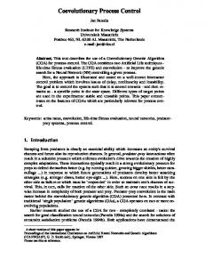
Figure 2. Spatial variation in host fitness caused by parasite burden. Left and right panels are for centre = 1 and 4, respectively. Missing values in left panel for migr = 0.001 are 1.70 and 1.77 for eigen = 3 and 4, respectively.
Coevolutionary dynamics
201
in fitness burden measured among patches. Since the CV is the ratio of the standard deviation to the average, I give a brief treatment of the average burden to establish the magnitude of the effect. Average burden is unaffected by noise in Design II; only 0.8% of the variance for 18 of a total of 431 degrees of freedom is explained by noise and its first-order interactions with migration, eigenvalue, and centre point. When the centre point is far from a boundary (centre = 4 in Table 1) then mutation has little effect, but when the centre point is near a boundary and migration is rare (centre = 1, migr = 1), local extinctions are important and mutation reduces the time that a type remains extinct in a patch (see below). The burden was therefore somewhat lower when mutation and migration were relatively low, and when the centre point was near a boundary. In Design II, when centre = 4, the average and standard deviation of the median burden within the twelve migration-eigenvalue groups is 0.423 and 0.059, respectively. The medians are nearly twice as high at centre = 1, which reflects the greater parasite burden that maintains a lower equilibrium abundance of hosts. The CV in host fitness among patches is presented in Fig. 2. Variation increases rapidly as the local dynamics pass from stable to unstable, as measured by the transition of the modulus of the dominant eigenvalue through the unit circle when eigen goes from two to three. Increased migration reduces the variation among patches, but the effects of local instability remain strong even under high migration rates. When migration is low and the centre point is near a boundary (left panel in Fig. 1), variation among patches is high because of occasional local extinctions of parasites (see below). An ANOVA on the logarithm of CV in Design II shows that migr, centre, eigen, and the first-order interactions between migr and the other two factors explains 64% of the total variance with only 20 of the 431 total degrees of freedom. The main effect of noise, with two degrees of freedom, explains an additional 7% of the variance. A single spatial sample provides nearly complete information about the average burden and the spatial variation in burden. Spearman's non-parametric correlation between a spatial sample and the long-term averages for the average burden and the logarithm of the CV in burden is greater than 0.98 when analysing the 432 runs in Design II. This suggests that the array of patches is in a temporally stationary condition with respect to these statistics even though host and parasite abundances are changing continually within patches. Extinction frequencies The location of the fixed point, centre, and the amount of migration, migr, are the primary determinants of extinction frequencies. Surprisingly, over the range of parameters studied, the mutation rate and the amount of noise have relatively little influence. To support these conclusions I will present a few results for extinction frequency for one of the two hosts and one of the two parasites when averaged over all 625 patches in each generation and over all 5000 generations of each run. The role of mutation can be seen in Design I. For centre = 1 and migr = 1 the median extinction rates over 12 runs are: for the hosts, 0.245 when there is no mutation and 0.238 when the mutation rate is 0.1; for the parasites, 0.422 when there is no mutation and 0.385 when the mutation rate is 0.1. For centre = 4 and migr = 1 the median extinction rates over 12 runs are: for the hosts, 0.005 when there is no mutation and 0.009 when the mutation rate is 0.1; for the parasites, 0.023 when there is no mutation and 0.010 when the mutation rate is 0.1. The median extinction rates are zero for all other treatment combinations when centre is 1 or 4. The role of noise can be seen in Design II. For centre = 1 and migr = 1 the median extinction rates over 12 runs are: for the hosts, 0.215 when there is no noise and 0.232 when the noise rate is 0.03; for the parasites, 0.514 when there is no noise and 0.454 when the noise rate is 0.03. For
202
Frank
centre = 4 and migr = 1 the median extinction rates over 12 runs are: for the hosts, 0.003 when there is no noise and 0.023 when the noise rate is 0.03; for the parasites, 0.039 when there is no noise and 0.096 when the noise rate is 0.03. The median extinction rates are zero for all other treatment combinations when centre is 1 or 4. The information in a single spatial sample about long-term averages of the extinction rates can be seen from the correlations between sample extinction rates and long-term average rates. In Design II, withi migr = 1 treatments, Spearman's non-parametric correlation coefficient between sample and long-term averages for hosts is 0.997 and for parasites is 1.0, with 144 observations for each coefficient. Temporal dynamics Introduction. The focus of this paper is on spatial variation in polymorphism and in successful attacks on hosts. The above results document the potential for extensive spatial variation among environmentally identical patches even when migration rates are high. The major processes affecting spatial variation are deterministic components of within-patch dynamics given in Equation 1, stochastic perturbations given in Equation 2, and migration. These three processes lead to global patterns in temporal dynamics. Loosely speaking, spatial variation may be maintained by temporal dynamics that are dominated by repeated local colonizations and extinctions or by stable limit cycles within patches that are out of phase among patches (Maynard Smith, 1974, Chapter 6). In an array of identical patches, mixtures of local extinctioncolonization cycles and stable limit cycles determine patterns of spatial variation. From a deductive point of view, the previous section documented that frequent extinction of types may be associated with high amounts of spatial variation, but that extinction is not a necessary condition for spatial variation. From an inductive point of view, all of the results have so far supported the idea that the long-term pattern can be assessed from a single spatial sample, including the frequency of extinctions. This agreement between the long-term pattern and a single spatial sample implies that the global distribution of types is at an equilibrium (stationary distribution) even though changes may be occurring in all patches in each generation. How much information about within-patch dynamics and the presence of stable limit cycles can be obtained from a spatial sample? I will present a series of plots to show that a surprisingly large amount of information about within-patch dynamics can be obtained from spatial data collected at a single point in time. Design. I have shown above that extinction frequencies are strongly dependent on the location of the fixed point determined by the treatment level of centre in Table 1. I therefore conducted two sets of runs: one at centre = 4, which should have low extinction rates, and one at centre = 1, which should have relatively higher extinction frequencies. For each centre point I examined three treatment combinations: (1) a dominant . eigenvalue associated with local instability and the potential for limit cycles, eigen = 4, low migration, migr = 1, and small amounts of stochastic noise, noise = 2; (2) as in (1) but with higher local perturbations caused by more migration, migr = 2, and more noise, noise = 3; and (3) as in (1) but with local stability, eigen = 1. These six treatment combinations, three for each centre point, were decided upon before any graphics had been observed for similar parameter sets. Each combination was run only once and the resulting graphics were used for the plots below, except for treatment (1) and centre = 1, in which a second run was used because it provided a better illustration of a key feature of the dynamics. Within each run, 2000 generations were completed without statistics being collected, then for
Coevolutionary dynamics
203
P 1
P 1
A B U N D A N C E
A B U N A N C E H1 ABUNDANCE
H1 ABUNDANCE
H 1
H 1
A B U N D A N C E
A B U N D A N C E
HO ABUNDANCE
HO ABUNDANCE
Figure 3. Spatial distribution and temporal dynamics of host—parasite abundances. The hash marks in the lower left corner of each plot locate the point at which abundance is zero. The maximum value in each dimension is a standardized abundance of one (Equation 1). The left column is the distribution from a spatial sample from 625 patches at a single point in time. The right column is the temporal dynamics of a single patch over 2000 generations. Treatment levels are centre = 4, eigen = 4, migr = 1, and noise = 2 (see Table 1). The HO—PO plots are very similar to the H1—P1 plots.
the following 2000 generations the sequence of host and parasite abundances were collected for a single randomly chosen patch among the 625 patches. These are the temporal data discussed below. The host and parasite abundances in each patch over all 625 patches were collected in a single spatial sample in the 3000th generation, the midpoint of the sequence of generations over which temporal data were collected. Low extinction rates. The results are plotted for centre = 4 and treatment combinations (1-3) in Figs 3-5. The left column in each figure shows the spatial data, and the right column shows the temporal dynamics in a randomly chosen patch. The top row shows the bivariate abundances for
204
Frank
P 1
1
A B U N D A N C E
A B U N D A N C E
H1 ABUNDANCE
H1 ABUNDANCE
H 1
H 1
A B
A B U N D A N C E
U N D A N C
HO ABUNDANCE
HO ABUNDANCE
Figure 4. Spatial distribution and temporal dynamics of host—parasite abundances. The treatments include more migration and noise than in Fig. 3 but are otherwise the same. Treatment levels are centre = 4, eigen = 4, migr = 2, and noise = 3. The HO—PO plots are very similar to the Hl—P1 plots.
one of the two host-parasite systems in each patch. The bottom row shows the bivariate abundances of the two hosts within each patch. These host-host dynamics determine patterns of polymorphism within and among patches. For centre = 4 and treatment (1), in which migration is low and the noise is small, the stable limit cycle is clearly seen in the top and bottom right (Fig. 3). Remarkably, the spatial data provide an almost perfect description of the temporal abundances. Note the rare local extinctions along the bottom of the upper left panel and along the boundaries of the lower left panel. The lower left shows the pattern of spatial polymorphism for hosts in the sample generation, in which Fs was 0.469. For centre = 4 and treatment (2) (Fig. 4), in which migration is much higher (0.05) and noise is twice as great, the patterns are similar to Fig. 3, but show greater perturbations. The clarity of the cycle under high migration and noise is striking. The lower left shows the pattern of spatial
205
Coevolutionary dynamics P
P 1
A B U N D A N C E
A
B U N D A
N C E 1 ABUNDANCE
1 ABUNDANCE
H 1
H
A B U N D A N
A
1
B U N A
N C E
C E O ABUNDANCE
O ABUNDANCE
Figure 5. Spatial distribution and temporal dynamics of host—parasite abundances. The treatments include lower eigenvalues than in Fig. 3 but are otherwise the same. Treatment levels are centre = 4, eigen = 1, migr = 1, and noise = 2. The HO—PO plots are very similar to the H1—P1 plots.
polymorphism for hosts in the sample generation, in which F„ was 0.427. The slightly lower F5 value compared with (1) is caused by fewer local extinctions. Last in this group where centre = 4, is the case of local stability under treatment (3) (Fig. 5). The results show the sort of local stability over time and global stability over space expected when extinctions are rare and the modulus of the dominant eigenvalue is within the unit circle. The lower left panel shows the pattern of spatial polymorphism for hosts in the sample generation, in which F5 was 0.046. High extinction rates. For centre = 1, local extinctions are expected to be much more frequent because hosts are kept well below their carrying capacity by parasite attack or disease. In treatment (1), local instability is expected, since eigen = 4, and migration and noise are both low. The upper left panel (Fig. 6) for spatial data on host-parasite abundances shows three types of
Frank
206
P 1
P
1 A B U N D A N
•
A B U N D A N C E
•
. .
C
•14e....4..
E
H1 ABUNDANCE
H1 ABUNDANCE
H 1
H 1
A B U N D A N C E
A B U N D A N •
C E
•• •nnn•.•
HO ABUNDANCE
HO ABUNDANCE
Figure 6. Spatial distribution and temporal dynamics of host—parasite abundances. The treatments include a lower centre point than in Fig. 3 but are otherwise the same. Treatment levels are centre = 1, eigen = 4, migr = 1, and noise = 2. The HO—PO plots for temporal dynamics has PO = 0 over all generations (local extinction), whereas the spatial plot is very similar to the H1—P1 plot.
patches: a clear outline of a limit cycle, data that indicate local stability near the centre point in some patches and, along the boundaries, local extinctions of the parasite in 52% of the patches and of the host in 30% of the patches. The temporal dynamics in the sample patch can be inferred from the right pair of panels. From the lower right panel, one or the other of the hosts was extinct most of the time, with a transition between the two extinction states. When HO went extinct, H1 was maintained near the equilibrium frequency by interaction with P1, which was also maintained with its density near the equilibrium point. The ball of points in the upper right is an equilibrium with the HO—PO pair extinct. These points are clustered near the fixed point and near where the cluster is in the centre of the limit cycle in the upper left. The lower left panel shows the pattern of spatial polymorphism for hosts in the sample generation, in which F5 was 0.814.
Coevolutionary dynamics
207
P 1
P 1
A B U N D A N C E
A B U N D A N C E
H1 ABUNDANCE
Hi ABUNDANCE
H 1
H 1
A B U N D A N C E
A B U N D A N C E
HO ABUNDANCE
HO ABUNDANCE
Figure 7. Spatial distribution and temporal dynamics of host—parasite abundances. The treatments include more migration and noise than in Fig. 6 but are otherwise the same. Treatment levels are centre = 1, eigen = 4, migr = 2, and noise = 3. The HO—PO plots are very similar to the H1—P1 plots.
For centre = 1 and treatment combination (2), local instability is still expected since eigen = 4, but migration is high (0.05) and noise is increased over treatment (1). The most striking result is that migration greatly reduces local extinctions and therefore stabilizes the limit cycle (upper left panel of Fig. 7) (Hamilton, 1986). Local extinctions in the spatial sample are less than 1% in this run. The lower left panel shows the pattern of spatial polymorphism for hosts in the sample generation, in which F5t was 0.430. For treatment (3) and the low centre point, with low migration and low noise, dynamics are locally stable but local extinctions are high (Fig. 8). The pattern of extinctions is most clearly seen in the lower left panel, which shows eight clusters of points — four in the interior and four along the boundaries with one or the other type extinct. The lower right shows a temporal transition
208
Frank P 1
P 1
A
A B U N D A N C E
B U N
D A N C
E
1 ABUNDANCE
1 ABUNDANCE
H
H
1
1
A
A B U N D A N C E
B U N
D A N C E
O ABUNDANCE
O ABUNDANCE
Figure 8. Spatial distribution and temporal dynamics of host—parasite abundances. The treatments include lower eigenvalues than in Fig. 6 but are otherwise the same. Treatment levels are centre = 4, eigen = 1, migr = 1, and noise = 2. The HO—PO plots for temporal dynamics has PO = 0 over all generations (local extinction), whereas the spatial plot is very similar to the Hl—P1 plot.
between two of these attracting clusters. In the spatial data, HO was extinct in 32% of the patches and H1 in 30%, with an F„ of 0.564 among hosts. Discussion Conclusions from the simulations Spatial variation. Coevolutionary dynamics can maintain high levels of spatial variation in polymorphism (Fig. 1). Spatial variation can be high even when successful migration is frequent and when there is no environmental cause of the spatial variation. These conclusions contrast with the typical beliefs that moderate amounts of migration will quickly reduce spatial variation in polymorphism and that the most likely cause of spatial variation in coevolutionary systems is
Coevolutionary dynamics
209
environmental variation among patches. Coevolutionary dynamics in an array of identical patches can also maintain high levels of spatial variation in the fitness burden of hosts caused by successful attack from parasites, herbivores, pathogens or predators (Fig. 2). The meaning of 'frequent' migration in this context may require clarification. Successful migration in these simulations implies that, in a fully populated patch, approximately 1% of the patch members in each time period (generation) are derived from propagules that immigrated in the previous time period. In traditional population genetic models, the absolute number of immigrants determines spatial variation (Slatkin, 1985). In those models, a few successful migrants in each generation is sufficient to prevent spatial variation. In the present model, successful immigration of 1% per patch may represent thousands or millions of new arrivals in each generation. Temporal dynamics: limit cycles versus extinctions and recolonizations. The spatially separate patches in the simulations are environmentally identical, and the parameters governing interactions are identical among patches. Patterns of spatial variation are therefore determined by the dynamics of changing abundances within patches that are out of phase among patches. Two types of spatial asynchrony contribute to spatial variation: stable limit cycles within patches that are out of phase among patches and repeated local extinctions and recolonizations. The simulations show that either or both types of spatial asynchrony may occur. For example, in Figs 3, 4, and 7, spatial variation is dominated by local limit cycles with phases that are uncorrelated spatially. In Fig. 8, local extinctions cause most of the spatial variation. In Fig. 6, both local extinctions and spatially uncorrelated local limit cycles contribute to spatial variation. Information in a spatial sample. The simulations have shown that data collected from several identical patches in a single spatial sample provide much information on both the long-term patterns of spatial variation among patches and the temporal dynamics within each patch. The simulations have assumed identical patch types and free migration (see below), so further work will be required to establish what can be inferred under different conditions and sampling schemes. As an example of estimating long-term pattern, the correlations between Fs, estimated from a single spatial sample and the average Fs, for a temporal sequence of 5000 spatial samples is greater than 0.98. For estimating temporal dynamics, Figs 3-8 show that each patch of a spatial sample is very much like a randomly chosen temporal sample from the dynamic history of a single patch. Spatial data contain this information because the temporal phase of the dynamics within a patch is weakly correlated among patches even with substantial amounts of migration. The potential for inferring temporal dynamics with spatial data may represent a substantial breakthrough for analysing evolutionary processes underlying the distribution and abundance of disease and herbivory. In the past, direct empirical studies of dynamics have usually not been very informative because of the long time course of evolutionary dynamics. Further considerations for empirical programs will be discussed below. Inferring temporal dynamics from spatial data is not a new idea. Darwin's (1984) analysis of the formation of atolls remains one of the most elegant examples. Applications in ecology have been discussed recently by Pickett (1989). The assumptions of identical patch types and free migration. In the simulations the environmental conditions and carrying capacity were the same for all patches. This assumption allowed the simulation results to show clearly that high levels of spatial variation can be caused solely by coevolutionary dynamics. The assumption of identical patch types is therefore conservative with respect to the claim for spatial variation in polymorphism.
210
Frank
Environmentally identical patches make it considerably easier to use spatial data for estimating the pattern of temporal dynamics within a patch. For example, if the variation among patches is caused primarily by environmental variability, then spatial variation provides no information about temporal aspects of coevolutionary dynamics. Any empirical information or statistical techniques that allow spatial variation to be partitioned into environmental and biotic components would be particularly valuable. The migration scheme in the simulations followed an island model (Wright, 1969). Under this model an immigrant is equally likely to have come from any patch; there is no correlation between distance and probability of successful colonization. Most population genetic and ecological models use this migration scheme. Alternative migration patterns include the steppingstone model (Kimura and Weiss, 1964), in which migrants come only from neighbouring patches, or the isolation by distance model, in which the probability of successful migration decreases with increasing distance (Wright, 1969). The free migration of the island model used in the simulations is likely to be the least conducive to the maintenance of spatial variation. The simulation has in this case used a conservative assumption. It is more difficult to produce a simple and general conjecture about the role of the migra\ion pattern in the maintenance of total polymorphism across all patches and in the patterns of extinction versus stable cycling. Relation to past work on overall population stability. Much research has been done on coevolutionary systems in patchy environments. Recent extensions and references to past work can be found in Sabelis and Diekmann (1988), Hanski (1989) and Pimm and Gilpin (1989). All of this work has focussed on stability conditions, that is, the conditions that are required to maintain a certain number of host and parasite or predator and prey species. The simulations described here extend or differ from this past work in three ways. (1) The present study focusses on the amount of variation among patches and the frequency of local extinctions rather than on the global existence of types. As far as I know, no other study has addressed these quantitative questions. (2) Past work has analysed systems with one predator and one prey species (e.g. Hilborn, 1975; Hastings, 1977). The present study extends the analysis of patch models to systems with two predator and two prey species. (3) Maynard Smith (1974, Chapter 6) noted that the migration pattern plays an important role in detefmining whether spatially distinct patches can cycle out of phase and thus contribute fo global maintenance of types. When migration is continuous and occurs over a shorter time scale than the life cycle, then migration tends to synchronize fluctuations in densities among patches. In this case of continuous migration, environmental patchiness cannot increase the probability that types are maintained. By contrast, if migration occurs discretely and, in effect, only a few times during the life cycle, then spatially distinct patches may have uncorrelated dynamics. Zeigler (1977) extended this analysis and provided a review of several related studies of discrete or continuous migration events and continuous Lotka–Volterra or similar dynamics. In the present study the discrete timesteps are equivalent for the life cycle and migration. Asynchrony among patches sometimes occurs in this discrete-time migration and discrete-time Lotka–Volterra model. Biological applications The Lotka–Volterra model in Equation 1 captures the general qualitative features of antagonistic coevolutionary dynamics. Recently, more realistic models have been developed for particular types of interaction which, for example, include recovery of a host type after infection by a
Coevolutionary dynamics
211
parasite and subsequent host immunity (Hassell and May, 1989). The specific assumptions that would extend Equation 1 to describe particular interactions would change the relationship between particular parameters, such as the intrinsic rate of growth, r, or host morbidity and mortality, m, and the eigenvalues of the dynamic system. In the extended models, the stability of local dynamics in each patch will still be governed primarily by the dominant eigenvalue of the system. Thus, the conclusions from the simulations presented here should apply generally, since they are based on generally applicable assumptions about migration pattern, spatial arrangement, and local dynamics as governed by the dominant eigenvalue. I briefly list some antagonistic coevolutionary systems, in which 'hosts' and 'parasites' have different interpretations. Within genomes, patrilineally inherited Y chromosomes and matrilineally inherited cytoplasmic genes are in conflict with autosomes over the allocation of resources to sons and daughters or pollen and ovules (Hamilton, 1967). In hermaphroditic plants, matrilineally inherited genes often cause pollen sterility, and this sterility can be suppressed by a variety of autosomal restorer genes. The complex antagonistic coevolutionary dynamics of cytoplasmic male sterility have been studied for single patches by Charlesworth (1981), Delannay et al. (1981), and Frank (1989). Some observations on spatial variation in cytoplasmic male sterility have been reviewed by Gouyon and Couvet (1985) and Frank (1989). Meiotic drive is another type of antagonistic genomic coevolution. In meiotic drive systems, one allele or supergene distorts the normal Mendelian segregation ratio and increases its transmission to offspring relative to its competing homologous allele (Zimmering et al., 1970; Crow, 1979). The action of the distorting supergene is often suppressed by alleles distributed throughout the genome – there is an antagonistic coevolutionary interaction between distorting complexes and genome-wide suppressors. Spatial variation in the array of distorting and suppressing genotypes is known within a few well-studied species (Hartl and Hiraizumi, 1976). Frank (1991b) and Hurst and Pomiankowski (1991) have suggested an important role of spatial divergence in meiotic drive for certain types of between-population and between-species hybrid sterility. Plant-pathogen interactions are one of the most clearly defined and best-studied types of antagonistic coevolution, in which particular host genotypes are resistant to a subset of the diverse array of pathogen genotypes known (Burdon, 1987). Burdon (1987, pp. 138-42) reviews data showing considerable spatial variation in disease resistance for several species. Most often, the spatial variation in genetics is attributed to climatic differences among locations. Climate probably plays an important role in spatial variation, but the results presented here suggest that significant spatial variation is to be expected even in an array of identical patches because of the continual dynamics from local cycles, extinctions and recolonizations. When genomic conflict interactions are added to the many parasites and pathogens that attack each species, it seems plausible that many loci throughout the genome are involved in an antagonistic coevolutionary dynamic system. Selection pressures are intense in genomic conflict and disease; in different patches these loci and the linked parts of the genome may be evolving rapidly and in different directions at any point in time. The contributions of such antagonistic coevolutionary dynamics to genetic diversity among populations and among recently diverged species has received little theoretical or empirical attention. When the different 'host' and `parasite' types are actually different species of host plant and different species of herbivore, or host insects and parasitoids, the conclusions concern spatial divergence of species composition and abundance. Testing hypotheses about dynamics Cycles. Hamilton (1980, 1982) has advocated the idea that stable limit cycles in the abundances of host and pathogen genotypes favour sexual over asexual reproduction. Assuming that particular
212
Frank
types of cycling can plausibly explain sex, how can one obtain empirical support for the widespread occurrence of such cycles? One approach to testing the role of pathogens in maintaining diversity and, indirectly, in favouring sex, has been to study the relative fitness of rare and common host genotypes in local populations. A condition likely to be necessary for stable limit cycles is that rare host genotypes will have an advantage over common genotypes because of relatively lower pathogen attack. Of two studies directly addressing this issue, one study found support for a rare-type advantage (Schmitt and Antonovics, 1986), whereas the other did not (Parker, 1989). Although such experimental studies provide valuable insight into the dynamics of hostpathogen interactions, they do not actually address the key issue for sex: temporal variation in the relative fitnesses of host genotypes. For example, suppose that the dynamic system of host and pathogen genotypes is at a stable equilibrium when all types are equally abundant. Then a rare-type advantage would be expected even if there were no tendency for temporal variation in relative fitnesses. To document repeated fluctuations in relative fitnesses of host types within a single patch would, of course, require a very long time. Worse, the results from the simulations suggest that a patch may be temporarily frozen in a fixed state with no cycling even when cycling and fluctuating fitness is typical of most patches at any one time. Thus, sufficient temporal samples can rarely be obtained for a single patch, and single patches are not necessarily good indications of typical dynamics. Alternative experimental and field approaches suggested by the simulations are discussed below. Spatial variation. Much recent work has focused on the forces that maintain genetic subdivision of populations (Slatkin, 1985). Roughly speaking, hypotheses for spatial variation tend to fall into two classes. First, selection is assumed to be a weak force and subdivision is dominated by migration, drift and mutation. Unless migration is rare, subdivision is expected to be low. Second, selection is assumed to be strong and to vary spatially and in a systematic way, yielding a cline in selection coefficients (Endler, 1977). Subdivision can be maintained in spite of high migration because of the strong selection. The simulations suggest a third hypothesis about the maintenance of spatial variation under relatively high migration (Maynard Smith, 1974, Chapter 6). Selection is intense for disease and resistance loci involved in the coevolutionary dynamic, but selection coefficients vary spatially in a manner that is partly uncorrelated with geography. The selection coefficients vary spatially and temporally because they are induced by an interaction between the fluctuating gene frequencies of hosts and parasites. The strong selection can overcome high migration rates and maintain spatial variation. Spatial variation in selection coefficients may be caused by asynchronous limit cycles or by continuing local extinctions and recolonizations. Experimental studies. Experimental laboratory systems can be used to test how coevolutionary dynamics and migration interact to determine patterns of local colonization-extinction, cycles and spatial variation and to test how much can be learned by spatial sampling. Considerable work has been done on coevolution between E. coli and the T bacteriophages in single 'patches' (Levin and Lenski, 1983; Lenski and Levin, 1985). In these studies the primary source of new genotypes in the patch is mutation. An extended design suggested by the simulations would allow simultaneous coevolution in many separate patches (e.g. chemostats) with various patterns of controlled migration between patches. Levin and Lenski (1985), and Lenski (1988) have discussed the possible roles in bacteria-bacteriophage coevolution of migration and local extinctions and recolonizations.
Coevolutionary dynamics
213
Field studies. Advances in technology will soon allow widescale screening of genetic variation in
natural populations. Study of nearly neutral loci could be used to establish patterns of gene flow and the colonization histories of patches. Simultaneous screening of particular resistance and virulence loci would allow separation of coevolutionary selection dynamics from the forces of migration and drift that would also be acting on the nearly neutral loci. Many useful DNA markers are likely to become available soon because of the economic importance of disease and herbivore attack on crop plants and the extensive genetic study of certain laboratory animals such as mice. The subdivided population structure of many mouse species may make this group a particularly good organism for future research. Sampling from many spatial locations over a few generations would provide the outlines of dynamical flow in the host-parasite interaction. For example, imagine that in the upper left panel of Fig. 3, instead of each point for a single sample there were beginning and ending frequencies within each patch. The plot would then be a set of arrows indicating the direction of change in abundances, or dynamical flow. Combined space-time data (Bennett, 1979) will almost certainly turn out to be the most powerful method for analysing coevolution in natural populations. Several theoretical, statistical and practical difficulties must be overcome before such studies could be accomplished and interpreted. Many lines of research are converging toward this goal.
Acknowledgements I thank R. E. Lenski and M. Slatkin for helpful comments on an earlier version of the manuscript. My research was supported by NIH grants GM42403 and BRSG-507–RR07008 and
NSF grant BSR-9057331.
References Bennett, R. J. (1979) Spatial Time Series. Pion, London. Burdon, J. J. (1987) Diseases and Plant Population Biology. Cambridge University Press, Cambridge. Charlesworth, D. (1981) A further study on the problem of the maintenance of females in gynodioecious species. Heredity 46, 27-39. Crow, J. F. (1979) Genes that violate Mendel's rules. Sci. Am. 240(2), 134-44. Crow, J. F. and Kimura, M. (1970) An Introduction to Population Genetics Theory. Burgess Publishing Co., Minneapolis, USA. Darwin, C. (1984) The Structure and Distribution of Coral Reefs. University of Arizona Press, Tucson. Delannay, X., Gouyon, P.-H. and Valdeyron, G. (1981) Mathematical study of the evolution of gynodioecy with cytoplasmic inheritance under the effect of a nuclear restorer gene. Genetics 99, 169-81. Endler, J. A. (1977) Geographic Variation, Speciation, and Clines. Princeton University Press, Princeton, New Jersey, USA. Frank, S. A. (1989) The evolutionary dynamics of cytoplasmic male sterility. Am. Nat. 133, 345-76. Frank, S. A. (1991a) Ecological and genetic models of host-pathogen coevolution. Heredity (in press). Frank, S. A. (1991b) Divergence of meiotic drive-suppression systems as an explanation for sex-biased hybrid sterility and inviability. Evolution (in press). Gouyon, P.-H. and Couvet, D. (1985) Selfish cytoplasm and adaptation: variation in the reproductive system of thyme. Verh. K. Ned. Akad. Wet. Afd. Natuurkd. Tweede Reeks 85, 299-319. Guckenheimer, J. and Holmes, P. (1983) Nonlinear Oscillations, Dynamical Systems, and Bifurcations of Vector Fields. Springer-Verlag, New York, USA. Hamilton, W. D. (1967) Extraordinary sex ratios. Science 156, 477-88. Hamilton, W. D. (1980) Sex versus non-sex versus parasite. Oikos 35, 282-90. Hamilton, W. D. (1982) Pathogens as causes of genetic diversity in their host populations. In Population
214
Frank
Biology of Infectious Diseases (R. M. Anderson and R. M. May, eds) pp. 269-96. Springer-Verlag, New York. Hamilton, W. D. (1986) Instability and cycling of two competing hosts with two parasites. In Evolutionary Processes and Theory (S. Karlin and E. Nevo, eds) pp. 645-68. Academic Press, New York. Hanski, I. (1989) Metapopulation dynamics: does it help to have more of the same? TREE 4, 113-4. Hartl, D. L. and Hiraizumi, Y. (1976) Segregation distortion. In The Genetics and Biology of Drosophila, Vol. 1B. (M. Ashburner and E. Novitski, eds) pp. 615-66. Academic Press, New York. Hassell, M. P. and May, R. M. (1989) The population biology of host-parasite and host-parasitoid associations. In Perspectives in Ecological Theory. (J. Roughgarden, R. M. May and S. A. Levin, eds) pp. 319-47. Princeton University Press, Princeton. Hastings, A. (1977) Spatial heterogeneity and the stability of predator-prey systems. Theor. Pop. Biol. 12, 37-48. Hilborn, R. (1975) The effect of spatial heterogeneity on the persistence of predator-prey interactions. Theor. Pop. Biol. 8, 346-55. Hurst, L. and Pomiankowski, A. (1991) A new explanation of Haldane's rule: causes of sex-ratio bias within species may also account for unisexual sterility in species hybrids. Genetics (submitted). Kimura, M. and Weiss, G. H. (1964) The stepping stone model of population structure and decrease of genetic correlation with distance. Genetics 49, 561-76. Lenski, R. E. (1988) Dynamics of interactions between bacteria and virulent bacteriophage. Adv. Microbiol Ecol. 10, 1-44. Lenski, R. E. and Levin, B. R. (1985) Constraints on the coevolution of bacteria and virulent phage: a model, some experiments, and predictions for natural communities. Am. Nat. 125, 585-602. Levin, B. R. and Lenski, R. E. (1983) Coevolution in bacteria and their viruses and plasmids. In Coevolution. (D. J. Futuyma and M. Slatkin, eds) pp. 99-127. Sinauer, Sunderland, Massachusetts. Levin, B. R. and Lenski, R. E. (1985) Bacteria and phage: a model system for the study of the ecology and co-evolution of hosts and parasites. In Ecology and Genetics of Host–Parasite Interactions. (D. Rollinson and R. M. Anderson, eds) pp. 227-42. Academic Press, New York. Levins, R. and Culver, D. (1971) Regional coexistence of species and competition between rare species. Proc. Natl. Acad. Sci. USA 68, 246-8. May, R. M. (1973) Stability and Complexity in Model Ecosystems. Princeton University Press, Princeton. Maynard Smith, J. (1974) Models in Ecology. Cambridge University Press, Cambridge. Parker, M. A. (1989) Disease impact and local genetic diversity in the clonal plant Podophyllum peltatum. Evolution 43, 540-7. Pickett, S. T. A. (1989) Space-for-time substitution as an alternative to long-term studies. In Long-Term Studies in Ecology. (G. E. Likens, ed.) pp. 111-35. Springer-Verlag, New York. Pimm, S. L. and Gilpin, M. E. (1989) Theoretical issues in conservation biology. In Perspectives in Ecological Theory. (J. Roughgarden, R. M. May and S. A. Levin, eds) pp. 287-305. Princeton University Press, Princeton. Sabelis, M. W. and Diekmann, 0. (1988) Overall population stability despite local extinction: the stabilizing influence of prey dispersal from predator-invaded patches. Theor. Pop. Biol. 34, 169-76. Schmitt, J. and Antonovics, J. (1986) Experimental studies of the evolutionary significance of sexual reproduction. IV. Effects of neighbor relatedness and aphid infestation on seedling performance. Evolution 40, 830-36. Slatkin, M. (1974) Competition and regional coexistence. Ecology 55, 128-34. Slatkin, M. (1985) Gene flow in natural populations. Ann. Rev. Ecol. Syst. 16, 393-430. Wright, S. (1969) Evolution and the Genetics of Populations, Vol. 2. University of Chicago Press, Chicago. Zeigler, B. P. (1977) Persistence and patchiness of predator-prey systems induced by discrete event population exchange mechanisms. J. Theor. Biol. 67, 687-713. Zimmering, S., Sandler, L. and Nicoletti, B. (1970) Mechanisms of meiotic drive. Ann. Rev. Genet. 4, 409-36.
Coevolutionary dynamics
215
Appendix In this appendix I sketch the method by which the parameters for Equation 1 were chosen for n = 2 given the centre point and the dominant eigenvalue. First some symmetry and general assumptions: c11 = C22 = 1 C 12 = C21 = C = r2 = r>0.02 si = S2 = S>0.02 = b 22 = bi >0 .02 b 12 = b21 = b20 .02 m12 = m21 = m2