Spatialized Audio Rendering for Immersive Virtual Environments Martin Naef1 1
Oliver Staadt2
Markus Gross1 2
Computer Graphics Laboratory ETH Zurich, Switzerland +41-1-632-7114
Computer Science Department University of California, Davis, USA +1-530-752-4821
{naef, grossm}@inf.ethz.ch
[email protected]
ABSTRACT We present a spatialized audio rendering system for the use in immersive virtual environments. The system is optimized for rendering a sufficient number of dynamically moving sound sources in multi-speaker environments using off-the-shelf audio hardware. Based on simplified physics-based models, we achieve a good trade-off between audio quality, spatial precision, and performance. Convincing acoustic room simulation is accomplished by integrating standard hardware reverberation devices as used in the professional audio and broadcast community. We elaborate on important design principles for audio rendering as well as on practical implementation issues. Moreover, we describe the integration of the audio rendering pipeline into a scene graph-based virtual reality toolkit.
CR Categories and Subject Descriptors: I.3.7 [Computer
Graphics]: Three-Dimensional Graphics and Realism — Virtual Reality Keywords: 3D Audio, Spatially Immersive Display, Virtual Reality
1. INTRODUCTION Virtual environments have steadily gained popularity over the past decade. With the availability of increasingly powerful graphics hardware, it is possible to drive virtual reality applications on platforms ranging from desktop-based systems to spatially immersive displays (SIDs) [5, 18, 26]. Research in the area of virtual reality displays has primarily focused on graphics rendering and interaction-related issues. In addition to realistic rendering and natural interaction, spatialized sound provides an important cue, greatly enhancing the sense of presence in virtual environments [2]. On the one hand, for small-scale desktop systems, standard PC audio hardware can readily be employed in combination with headphones or multiple speaker setups. Furthermore, programming libraries such as Microsoft’s DirectX [20] or Creative’s implementation of OpenAL [3] provide sufficient support for those setups. On the other hand, for large-scale SIDs, stereo headphones are often not feasible and these APIs cannot provide the necessary flexibility with regard to the number of speakers mounted at arbitrary positions. High-end audio systems [17] can provide flexible hard- and software solutions with good scalability. Unfortunately, these solutions can significantly increase the total cost for building an SID. Permission to make digital or hard copies of all or part of this work for personal or classroom use is granted without fee provided that copies are not made or distributed for profit or commercial advantage and that copies bear this notice and the full citation on the first page. To copy otherwise, or republish, to post on servers or to redistribute to lists, requires prior specific permission and/or a fee. VRST'02, November 11-13, 2002, Hong Kong. Copyright 2002 ACM 1-58113-530-0/02/0011…$5.00.
We are currently developing a novel networked SID, the blue-c, which combines immersive projection with multi-stream video acquisition and advanced multimedia communication. Multiple interconnected portals will allow remotely located users to meet, to communicate, and to collaborate in a shared virtual environment. We have identified spatial audio as an important component for this system. In this paper, we present an audio rendering pipeline and system suitable for spatially immersive displays. The pipeline is targeted at systems which require a high degree of flexibility while using inexpensive consumer-level audio hardware. For successful deployment in immersive virtual environments, the audio rendering pipeline has to meet several important requirements: • 3D localization: The accurate 3D positioning of the virtual sound source is of crucial importance for spatial sound. The perceived position of the sound source should match the spatial location of the associated object in the virtual environment. The main challenge here is to map sound sources at arbitrary virtual positions to a limited number of speakers, whose real position is often constrained by the physical setup of the SID. • Room simulation: Acoustic room simulation provides an impression of important properties of the virtual environment, e.g., the size of a virtual room, the reflection properties of the walls, etc. • Live audio input: In addition to synthesized sound, live audio input is important for applications in collaborative virtual environments. Sound input can either be local or can be received over the network from a remote portal. • Speed and efficiency: There is a trade-off between accurately simulating underlying physical properties of spatial sound and the efficient realization of a sound rendering pipeline using standard hardware. It is important to allow for a reasonable number of simultaneous virtual sound sources. The audio rendering pipeline presented in this paper meets these requirements. This is achieved by efficiently simulating important acoustic phenomena in software. While we cannot model exactly all physical properties of spatial sound, we use simplified, but proven [1] models that produce convincing results. Additional realism is achieved by adding reverberation using an external hardware device. This paper shows how these algorithms are integrated into a sound server that fits well into our scene-graph based virtual reality application programming toolkit and which requires only moderate processing power, providing up to 37 localized sound sources on a single 400 MHz MIPS R12000 processor. The sound server is integrated into the core of the blue-c software environment, making it easy to use and providing tight synchronization with the graphics system.
2. RELATED WORK Simulating acoustic phenomena is a well documented research area. There is a variety of systems, ranging from simple 3D positioning of sound effects up to complex, physics-based simulation of concert halls. Solutions that render soundtracks offline in parallel to computer graphics have been available for many years [28, 30]. For interactive, immersive virtual reality, the audio system must render all sounds in real-time. Sound systems for spatially immersive displays [5, 8], however, have some specific requirements that are not easily met by existing standard solutions.
VR Audio Systems. Software toolkits for immersive virtual
reality environments typically provide some kind of audio rendering subsystem. Avango [29], for example, uses a sound server [8] based on the MAX/FTS sound processing system [7]. It is controlled over the local network via UDP. Integration into the scene is accomplished with special nodes in the scene graph. IRCAM’s Spat modular sound processing software [15], which is available as a MAX/FTS object, implements a pipeline similar to ours. It is not clear, however, how it can be integrated into our virtual reality application development system with dynamically moving sources, networked audio streams, and how many sound sources can be spatialized in real-time without dedicated DSP hardware. The DIVA system provides sophisticated synthesis and spatialization algorithms [14]. Its high-quality spatialization however requires offline-processing. The CAVERNSoft G2 toolkit [19] includes tools for streaming audio data over the network, however, it does not provide support for spatialization.
3D Localization. There are two basic approaches for localizing
sound sources: Volume panning with or without crosstalk-cancellation [22] and filtering with a head related transfer function (HRTF) [12]. Volume panning methods model a sound field with different intensities according to the direction of the virtual source. They achieve good localization precision if there are enough speakers available [24]. Using a large number of speakers allows for simulating sources with high precision using wave field synthesis methods [27]. HRTF-based approaches model the frequency response of the human head and ear as a function of the source direction. This approach is especially suited for sound reproduction through headphones. Using HRTFs with speakers is possible, but it requires careful crosstalk-cancellation to achieve good localization precision [22]. Unlike our solution, systems based on HRTFs must be adjusted for the individual user and require head-tracking when using headphones. 3D localization using volume panning is implemented in most toolkits targeted at the multimedia and game market, such as Microsoft’s DirectSound [20], Creative Lab’s EAX or OpenAL [3]. Hardware-acceleration for these interfaces is available in consumer hardware. These systems rely on standard quadraphonic or home-theater 5.1 surround speaker placement and provide only minimal localization in the Z-axis by attenuating or amplifying the high frequency components of the signal. Such a fixed speaker positioning scheme prohibits the use of these audio APIs in a SID with large, solid projection walls in front and to the sides of the user. Other reasons against using low-end consumer-level hardware are the lack of sample clock synchronization when more than two input channels are needed, and the lack of customizable insertpoints in the signal path, e.g., for adding customized reverb algorithms. Our system supports arbitrary positioning of the speakers. High-end algorithms add early reflections for additional localization and distance cues [14, 17]. These reflection patterns are cal-
culated from a simplified environment geometry that is provided to the system. The audio signal is then convolved with this impulse response. High-end systems, such as Lake’s AniScape or SpaceArray [17], are typically equipped with dedicated DSP hardware to provide the necessary processing power for these calculations. In a typical back-projection setup, large projection walls made of glass form a bad acoustic environment with many reflections. These reflections and resonances interfere with the simulated responses, rendering the additional effort and costs questionable. Ambisonics [13, 9] B-format provides an encoding scheme that allows full 3D localization of sound signals with four discrete channels. It can be made compatible with standard two or 5.1 channel equipment (UHJ hierarchy and G-format, respectively) where it provides an improved stereo or surround experience. Although it was used in the music industry, Ambisonics encoders and decoders never became a commodity.
Room Response Simulation. Simulating the acoustic room response is essential for a realistic sound environment. The level, time, and density of early reflections and the reverb tail provide an impression of the size, form and materials of the surrounding environment. From daily experience, we know that the response of a small bathroom sounds significantly different than that of a large church. Even though we may not be consciously aware of these acoustic properties, we immediately notice when something is wrong. Physics-based simulation of acoustic properties is available for architectural design (http://www.netg.se/~catt/), especially for concert halls. These systems calculate the room response for a given position and sound source and then convolve audio streams. Calculating the impulse responses using ray-tracing methods [16, 23] is a very time consuming offline process and therefore not suited for interactive virtual environments with a moving listener and several moving sound sources. Recent approaches using prioritized beamtracing [10, 21] are promising. Once they model some additional frequency-dependent effects in real-time, they will probably provide pleasing and realistically sounding results, given enough available processing power. Applying long impulse responses with low latency is still computationally expensive, though. Real-time convolution systems using low-latency “block-wise” FFT are available for both musical applications or simulation purposes [17]. These are either limited to a small number of sound sources and/or prohibitively expensive. Especially with physical simulation approaches, there is always a trade-off between available DSP-power and achievable realism. Dedicated parallel processing systems are used for high-end simulation and training applications where precise auditory cues are required. For the music and film industry where a pleasing sound is more important than perfect realism, generalized reverberation algorithms that can be parametrized with room size, characteristics of early reflections and the reverb tail are used to provide the illusion of a natural environment. The algorithms typically use nested networks of allpass-filters with feedback [11, 6], the implementation details are usually considered a trade secret, though. These algorithms require significantly less processing power to achieve a pleasing result compared to physics-based simulations. We choose this approach because it fits our target applications best (see Section 4.6). Current low-end sound hardware targeting the game market includes similar reverberation algorithms. Due to limited processing power, they often produce “metallic” sounds and introduce artefacts such as unwanted modulation and pitch changes in the reverb tail.
3. SYSTEM OVERVIEW
Source
Figure 1 depicts a high-level overview of the blue-c VR system. Application data is maintained in a scene graph, which contains both graphics and audio nodes. The scene graph, which can dynamically be modified by the application, is traversed independently by the graphics and the audio sub-systems. Synchronous rendering of virtual objects and virtual sound sources is achieved by providing feedback from the graphics sub-system to the application (see Section 6). Application
sync
Graphics System
Source
1
Distance Gain 3D Positioning Reverb
Room-EQ
LPF
Speakers
Sub
Head Tracking
Figure 2: Audio rendering pipeline.
Sound System
1
Air Absorption
Projection Graphics Pipeline
Scene
Distance Delay
Mix Bus
1
Localization Pipeline
n n
n
Reverb n
Figure 1: System overview including scene graph, graphics and audio rendering subsystems. The audio rendering sub-system comprises four core functional units: • The sound sources are controlled by scene graph nodes or by the application. They provide audio samples and keep all information that is required for localization. • The localization pipeline receives data from the sound sources. The data is delayed, filtered and split to the output channels according to the positional information from the source. The localization pipeline subsequently sends information to the reverb send channel. • The reverb unit generates the room response. The data stream received from the localization pipeline is processed and sent to the mix bus. • The mix bus sums all incoming data. After clipping, the data is sent to the digital-to-analog converter which feeds the speakers and subwoofer. We follow a volume-panning-based localization approach with multiple speakers that can be implemented using inexpensive, offthe-shelf hardware components. Even though head-tracking information is typically available in SIDs, we want to avoid that the user has to wear other devices, such as headphones, in addition to stereo glasses. We also avoid the adjustment of HRTF data for different users.
4. THE AUDIO RENDERING PIPELINE In this section, we construct a pipeline for spatialized audio rendering. This pipeline comprises all important functional stages, including audio sources, distance delay, air absorption, distance gain, and 3D-positioning. Figure 2 depicts the entire pipeline in detail.
4.1 Audio Sources Input audio data can originate from four different types of sources:
• Prerecorded audio can be loaded into memory or streamed from disk. Background music or long audio loops are typically streamed, short and repeatedly used sound effects are preloaded to reduce the number of operating system calls and the overhead of sampling rate and format conversion. • Live input is used to integrate external sound sources. This includes microphones, external hardware synthesizers for music or effects, or other sound sources. • Networked input receives an audio data stream over the network. • Synthesized audio may be used for sound effects or music. Each audio source includes position, global gain and reference distance information. The reference distance is used for adjusting the gain and air absorption according to the actual distance between the object and the listener. The distance from the object to the listener defines where a gain equal to one reproduces the signal at correct loudness. All audio sources must provide data with the system sampling rate and data format. The conversion is provided by the audio file libraries [4]. The sampling rate of the input system should be synchronized to the output system to avoid drop-outs due to clock drifts.
Audio Buffers. All audio data is processed in blocks with a con-
figurable length, typically in the order of 20 ms. This length defines the maximum update latency because new calculation parameters are only set at block boundaries. The audio block length should be choosen roughly equal to or slightly higher than the frame time of the graphics system to achieve a similar delay for scene-updates in both the visual and the sound rendering. Shorter blocks are less efficient to process, especially for audio sources that stream data from disk. Furthermore, they do not provide a smooth parameter interpolation for moving sources, resulting in a continuous stop and go motion because the target position values are set once per graphics frame only (see Section 6.3). If the blocks are too long, there is a noticeable delay between user interaction and the sonic feedback. The size of the audio rendering blocks is always rounded up to the next 16 sample boundary to fit nicely into the system cache and to allow for loop-unrolling optimizations. Audio buffers are managed by the main sound service. They are reused to avoid the cost of dynamic memory allocation or wasted space due to barely used buffers. All data is kept as channel-interleaved 32 bit floats.
4.2 Distance Delay and Doppler Effect
4.4 Distance Gain
The low propagation speed of sound results in perceivable delays for distant events and the Doppler effect, a frequency shift for fast moving sources. Both effects can be modeled by delaying individual sound samples as opposed to delaying trigger events and modeling the Doppler effect with a vary-pitch sound source, which, however, is not practical for live and networked input. The delay time is given by
In this step, the gain for the source is calculated as a function of Ds:
Ds t d = ------------ , v sound
(1)
where Ds is the distance from the source to the listener and vsound is the speed of sound. Audio samples are delayed by storing them in a delay line buffer. A new data block is added into the delay line buffer at the current position Pcur as shown in Figure 3. Data is read in blocks starting at P cur + t d.last and ending at P cur + t d . Then, P cur is advanced to the next block and td.last is set to td. The number of samples read and written remains constant for each simulation step. The read position is interpolated linearly for every sample and samples are read at fractional positions with linear interpolation. Pcur+ td+ tblock
Pcur+ td.last
Pcur+ tblock
Pcur
Delay Line
Read Data
Write Data
Figure 3: Delay line with block read and write. The time difference between t d.last and td results in a sweep across the data, producing the Doppler effect. Note that fast moving sound sources should not include excessive high frequency components as anti-aliasing filters are not applied for performance reasons. The distance delay line is organized as a circular buffer. It holds 218 sample frames by default which equals to roughly six seconds worth of audio at 44.1 kHz sampling rate and allows to model objects at a distance up to 2 km. Distances exceeding this limit are clamped to the maximum. The delay line length could be shortened for smaller environments if the available memory is constrained.
4.3 Air Absorption In addition to the regular media-independent power loss, we also model the high-frequency damping effect of the air. The energy dissipation in air only affects frequencies above 1 kHz with approximately -4 dB damping per km. This effect is approximated by applying a standard bi-quad filter with highshelving characteristics. The distance is rescaled using the reference distance to avoid excessive filtering. The filter coefficients are not interpolated within the block size. This is a reasonable simplification as long as block sizes are kept reasonably short. More sophisticated simulations, taking humidity and other environmental factors into account, provide little advantage for our applications at a much higher computational cost. As a welcome side-effect of the air absorption filter, high-frequency aliasing-noise from the Doppler effect simulation is attenuated during this step.
D ref L d = --------, Ds
(2)
where Dref is the reference distance. It models the intensity fall-off according to the distance for point sources.
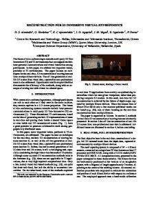
4.5 3D Positioning Up to this point, all audio data were treated as a single channel stream. In the 3D positioning stage, the stream is mixed onto several speaker channels. The normalized vector vs pointing from the listener to the source defines the direction of the source. This direction must be reproduced as closely as possible using a limited set of speakers. In a possible implementation, each speaker defines a vertex of a convex hull of triangles around the listener. The system calculates the intersection point and triangle between the convex hull and the ray defined by vs. The signal is then distributed to the three speakers at the triangle vertices according to their distance to the intersection point. This method works well even with a small number of speakers as long as the listener stays inside the convex hull. Our optimized method is based on the ideas presented in the VBAP method [24]. The dot-product between vs and the vector to the speaker vspk defines the gain. Negative results, i.e., speakers with an angle to the source larger than 90 degrees, are set to zero, disabling the respective speaker for the current source. To avoid large differences in the perceived spread between sources lying exactly in the direction of a speaker and sources between speakers, we increase the active angle for each speaker by adding a bias of 0.1 and rescaling the dot product. The channel gain for each speaker is therefore given by:
v spk ⋅ v s + 0.1 L chn = max --------------------------------, 0 , 1.1
(3)
where . denotes the dot product. This means that speakers slightly behind the plane defined by the listener and the source direction may be active too, providing more constant spread perception. The resulting channel gain vector is then normalized to guarantee constant power regardless of the number and position of the speakers. This CPU efficient vector-based panning method works well if there are enough speakers available to cover all angles. Eight speakers located in the corners of a cubic projection environment provide a very good coverage, even without a final normalization step. For typical virtual worlds with a bias on events in front of the listener, six speakers still provide good coverage. Figure 4 illustrates the possible speaker placement in our projection environment.
4.6 Reverb Processing Up to this stage, the pipeline provides a simulation of a single sound source without environment interaction. Such a “dry” source will never sound natural without simulating the room response though. There are two fundamental methods for generating room responses: Calculating the reflection patterns using physical simulation and convolving the audio signal, or using general parametrized algorithms that generate a realistic experience. For our system, we decided to use high-quality implementations of param-
(a)
Source
(b)
Distance Delay Air Absorption g
f
Mix Matrix
3D Positioning
Rev.
Figure 4: Possible positioning of speakers in the blue-c: (a) Six speaker setup. (b) Eight speaker setup. etrizable algorithms that can be found in studio effect processors for the music industry. The typical applications for our system are located in fictional, often highly abstract places where simulation has limited meaning and where an intuitive reverb description including decay times, pre-delays and damping factors is convenient for the designer. This saves us a complex simulation and a lot of processing power at the cost of some added latency due to the use of an external reverb unit. The reverb processor is fed through a send bus which is kept in parallel to the speaker bus. The output of the reverb system is then mixed onto the speaker bus. Each sound source includes a reverb send level parameter to control its contribution to the overall reverb simulation. We control the effects unit using a MIDI connection. The effects processor should support smooth parameter interpolation to avoid clicks when changing room parameters. The room response not only provides a realistic impression of the environment, it also provides an additional distance cue. Sources close to the listener have a high direct sound to room response ratio, whereas the room response is the dominating component for far away sources. We approximate this effect by reducing the reverb send level Lrev for audio sources that are close to the listener according to:
D ref 2 L rev = 1 – -------------------- . D s + D ref
(4)
4.7 Loudness Projection The loudness projection is the last step before the final mixdown. The distance between the listener and the speakers must be taken into account. This is especially important in immersive environments where the user can freely walk around. The tracked head position is used to update both the speaker direction vectors and individual speaker gains. The gain is defined by
D spk L spk = --------------- , D spkref
(5)
where Dspk is the actual speaker distance and Drefspk is the speaker reference distance. The speaker reference distance is defined to be equal to one meter for simplicity.
Room-EQ
LPF
Speakers
Sub
Figure 5: Illustration of the fused pipeline. A mixdown matrix M defining the gain factors for each target channel is calculated once per block using the information stored in the 3D positioning service. The output channel elements include the normalized gain from the positioning stage Lchn multiplied by the correction factor for the current listener position Lspk. Furthermore, each element is multiplied by the overall gain factor of the object Ls and distance gain Ld, resulting in
M i = L chn ⋅ L spk ⋅ L d ⋅ L s ,
(6)
where i is the index of the output channel. The dedicated low frequency effect channel is set to L d ⋅ L s , ignoring positional information (see Section 4.9). The mixdown matrix also includes the reverb send channels. These entries are set to the source gain factor Ls multiplied by the distance gain Ld and the reverb send level Lrev according to (4):
M i = L rev ⋅ L d ⋅ L s .
(7)
Unused channels are set to zero in the mixdown matrix. For the mixdown, each input sample is multiplied by a temporary mixdown matrix, the resulting vector is added to the main mix bus. The temporary mixdown matrix is a linear interpolation between the last mixdown matrix and the matrix calculated for the current block. This results in smooth changes of the channel gains, avoiding clicks and loudness jumps when the position or master volume of the audio source has changed. As a performance optimization, the interpolated mixdown matrix is recalculated every 32 samples only. The use of the mixdown matrix fuses the 3D positioning, loudness projection and reverb send operations into a single, efficient operation. In theory, more operations could be included into the mixdown-step, in practice, however, the large number of temporary values needed for interpolation and filter coefficients would defeat efficient processor register allocation. Speaker configuration, normalized listener to speaker vectors vspk, and the loudness projection factors Lspk are cached in the 3D positioning service. This information is updated once per audio rendering cycle. The current head position is read from a tracking system.
4.8 Fused Pipeline
4.9 Equalization and Low Frequency Management
Some of the highly modular functional stages can be combined to yield a streamlined pipeline that can be implemented efficiently without the loss of functionality. The last stages of the rendering pipeline, including distance gain, 3D-positioning and loudness projection, are fused into a single mixdown matrix representation, reducing the localization pipeline depth to three stages as shown in Figure 5.
Before the sound is sent to the speakers, an optional bank of equalizer filters is applied to the audio stream. This filter bank is used to compensate for the non-linear frequency response of the speaker system and to attenuate resonant frequencies of the acoustic environment. An additional audio channel contains the sum of all speaker channels. This channel is low-pass filtered and sent to a subwoofer,
providing additional bass-response. The bass cross-over frequency is configurable. Typical values range between 50 and 100 Hz, depending on the speakers and subwoofer used.
4.10 Handling of Non-spatialized Sound Not all audio sources are spatialized. For example, background music used as theme for certain environments should be rendered without further processing. Sound sources without positional information are treated similar to localized sound sources but without the delay and air absorption filtering. The sound is distributed to the speakers with the global volume level applied only.
5. IMPLEMENTATION The audio system consists of the main service, a 3D positioning service, a generalized audio source class with three derived implementations and some helper classes as shown in 6.
ital media library was used for communication with the audio hardware and audio file input. It provides all necessary sample rate and data type format conversions. We used an Alesis AI-3 eight channel AD/DA converter, which is connected directly to six Yamaha MSP5 powered speakers and to a Yamaha SW10 subwoofer, the reverb unit, a wireless microphone system and a CD player. We used a t.c. electronic MONE XL studio effects processor for the reverberation system. External audio input was provided by a wireless microphone system and a CD player.
6. INTEGRATION INTO THE BLUE-C API This section describes the integration of the sound rendering service into the bcAPI, our blue-c application programming interface. The bcAPI provides easy to use mechanisms for implementing collaborative, immersive virtual reality applications.
6.1 API Concept PreloadData
SoundService
LiveInput
3DPositioning
ReverbControl SoundSource
StreamSource
PreloadSource
LiveInputSource
Figure 6: Sound service class model. The main service initializes the audio I/O hardware, keeps a list of active sound sources, runs the rendering loop and provides a high-level interface for the application. It also instantiates the 3D positioning service which keeps a list of speakers and their relative position to the tracked user. It gets the head position from a tracking service. The audio source objects implement the full rendering pipeline, derived classes implement audio streaming from file, memory or live-input. The reverb control class provides a driver interface to the external reverb unit.
5.1 Process Model The implementation of the fused pipeline was optimized to run in a single process on an SGI Onyx 3200 graphics server. This process calls all audio sources to mix a single buffer down to the main bus, then blocks until the hardware is ready to accept the buffer. Parallelization by providing additional mix busses with their own processes would be straightforward, but it would take away processing power we need for the graphics rendering and provide more sound sources than is needed in practical applications. Accessing and updating audio source parameters can be done from any process. The audio source objects avoid conflicts by using locking mechanisms. The rendering pipeline always uses the most recent values and interpolates from the state active at the end of the previous rendering block, providing smooth level and position transitions.
5.2 Hardware and System Libraries We first validated the algorithms using a PC running Windows 2000 with an eight channel audio interface. The optimized, fused implementation runs on a Silicon Graphics Onyx 3200 with eight 400 MHz MIPS R12000 processors and the standard eight-channel ADAT digital audio interface. The SGI dig-
The bcAPI consists of a system core object which keeps a list of services and the main data structure, the scene graph. Input services can either provide state information through public methods or generate messages which are passed to the application or other services. Services are started and initialized according to a configuration file. Available services include a multi-pipe graphics rendering system, X11 device input, a magnetic tracking system for the head and 3D interaction devices, a sound service, and others. The scene graph is the main data structure. It is based on SGI OpenGL Performer v2.5 [25]. The scene contains traditional 3D geometry as well as custom nodes for rendering remote users, freeform curves and surfaces, dynamic particle systems, video inlays and active nodes for behavioral data. A blue-c application registers the main application class with the core. This class provides a set of methods which are called by the core. These methods include application startup, per-frame processing, message-handling and shutdown. In these callback methods, the application may modify the scene-graph as a reaction to messages or during the regular frame processing and call system services. Additional callbacks can be registered for customized graphics rendering. The integration of the audio rendering system into the blue-c API consists of two main components: The audio rendering service and active control objects in the scene graph.
6.2 Sound Service The sound service provides a low-level interface for playing back sounds in our environment. A forked process configures the audio hardware according to the settings defined in a configuration file and renders audio source objects. Configurable options include the number of output channels, number and position of speakers, block length, default path to audio files, and reverb unit driver and setup. All audio source objects are created and managed through methods provided by the sound service. Whenever a new sound source is created, a handle to the source is returned to the application. This handle is used for updating parameters such as position or master gain of the sound object. The sound service also keeps a list of preloaded audio objects. These are identified by an integer handle and include all samples already converted into the internal audio representation for efficient playback without disk access. The sound service is also responsible for audio input. It reads data from the configured audio source. Input channels can be
named for ease of use and portability across different target systems. Names are defined in the configuration file. The input system is also used for retrieving the reverb output from the external effects processor. The sound service is not aware of data in the scene graph or the active view into the virtual world. All positional information is expressed in the same metric, right-handed, Z-up, real-world coordinate system that is also used by the other hardware interface services.
6.3 Audio Nodes The application can choose to talk directly to the sound service. This is the preferred way for sound effects as immediate reaction to events generated by input devices. A more elegant way is to include active audio nodes directly in the scene graph for all other sounds. Active nodes are special nodes in the scene graph that can be placed anywhere in the hierarchy. Active nodes are evaluated once per frame, providing a single synchronization point. They can update service or scene graph parameters and trigger events based on the position of the viewer relative to the origin or area defined by the node. Both evaluation and trigger callbacks are defined as virtual members and can be provided by the application developer for customized active area management such as automatically opening doors. The API provides a set of active node implementations for controlling the audio system. They start or stop a defined sound whenever the distance between the object origin and the user crosses defined thresholds. This works for both localized and non-localized sound sources such as background music. For localized sound sources, the position of the sound source is updated for each frame to the corresponding real-world coordinates. Sound sources therefore automatically follow objects in the scene if their corresponding control node belongs to the same transformation group, e.g., if they are children of the same group transformation node. The same active node concept is also used to control reverberation parameters. Whenever the user enters a defined area, the external effects processor is reprogrammed to simulate rooms of a defined size or material.
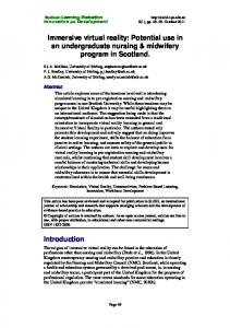
7. EXPERIMENTS We validated the localization algorithms with several experiments. All experiments were done on an SGI Onyx 3200 (see Section 5.2) running applications built using the blue-c API presented in Section 6. The audio clock rate was set to 44.1 kHz. The block length was set to 20 ms to meet the typical graphics rendering frame rate of 50 Hz. Reducing the block length to 10 ms did not result in relevant performance differences. Figure 8 shows the first blue-c projection environment with six speakers installed.
Figure 8: Setup of the blue-c with six speakers.
Localization. Localization precision and intensity distribution was first tested by slowly moving a virtual sound source around the listener on a sphere. No obvious “holes” were present with the six speaker configuration. Simulations indicate that near constant localization precision would be achievable with eight speakers. The next experiment was to seek moving ships emitting engine sounds in a misty environment with a rather short visibility range but high sound levels (see Figure 7). It was easily possible to find the scattered ships based only on auditory cues. Localized audio events can help to draw the user’s attention towards occluded areas in a virtual world. This is a powerful tool for the designer of the virtual environment to guide the user.
Reverberation. Reverberation mainly depends on the effects processor used and the appropriate parametrization by the designer of the virtual environment. We tested the implementation with an indoor scene consisting of two rooms with different reverberation parameters. Even without a physically correct simulation, the reverberation provided the user with an additional impression of the space.
7.1 Performance Measurements The performance of the system was measured in number of concurrent sound sources that can be active at the same time. The sound sources were tested with mono and stereo input and with activated localization. The localization tests were done with a mono source. For the preload data, we used a looped source with 320,000 samples. The streaming sources loaded a long wave file from a local disk. It was recorded in 44.1 kHz 16 bit format, sample rate and format conversion was done on the fly. The live-input tests were performed with a mono microphone source and a stereo CD input. The results presented in Table 1 tell the maximum number of sound sources that could be activated without signal drop-outs. Table 1: Maximal number of sound sources. Source
Figure 7: Screenshot of the ship seeking test application.
Mono
Stereo
Localized
Preloaded
78
33
37
Live input
54
25
30
Streaming
65
31
33
Disabling the distance delay stage significantly increased the maximal number of available sources, approaching almost the performance of non-localized sources. Increasing the system sample rate to 48 kHz reduced the numbers for preloaded and live input by
about 5%, whereas streaming performance dropped significantly due to the necessary sampling rate conversion.
7.2 Application Scenario The sound rendering system is used to enhance a virtual museum demonstration application. Whenever the user approaches an exhibition object or picture, a recorded explanation text is played from the position of the object. The playback stops if the user walks away. Figure 9 shows rendered views of the scene with a visualization of the active sound regions in the form of spheres. Additional sound sources are present for water noises from the fountain in the center, a non-localized background loop and a welcome message in the entrance door.
(a)
(b)
Figure 9: Active sound regions in the virtual museum depicted as red spheres. (a) Top view. (b) Visitor’s view.
8. CONCLUSIONS AND FUTURE WORK In this paper we presented a system for audio rendering for spatially immersive displays, integrating efficient, proven algorithms into a sound server that fits well into our scene-graph based application programming environment. We achieved a reasonable tradeoff between localization precision, realistic room acoustics and computing power required by using simplified, physics-based models and integrating an external studio effects processor. We also included tools to deal with shortcomings of the acoustic environment formed by the SID. The system is completely built using affordable standard hardware components. Future work will include porting the sound rendering service to a dedicated PC. The service will then be controlled remotely over the network. Directional sound sources will be implemented, accounting for different sound emission characteristics depending on the angle of an object towards the listener. An area management system is currently under construction and will be used for both visibility culling and occlusion and doorway simulation for sound sources.
ACKNOWLEDGEMENTS We would like to thank Edouard Lamboray for proofreading, Erich Crameri for his prototype implementation, and all members of the blue-c team for many inspiring discussions. This work has been funded by ETH Zurich as a “Polyprojekt” (grant no. 0-23803-00).
REFERENCES [1] D. Begault. 3-D Sound for Virtual Reality and Multimedia. AP Professional, 1994. [2] J. Blauert. Spatial Hearing: The Psychoacoustics of Human Sound Localization. MIT Press, revised ed., 1997. [3] Creative Technology Limited. Creative OpenAL Programmer’s Reference 1.0, 2001.
[4] P. Creek and D. Moccia. Digital Media Programming Guide. Silicon Graphics, Inc., 1996. [5] C. Cruz-Neira, D. J. Sandin, and T. A. DeFanti. Surround-screen projection-based virtual reality: The design and implementation of the CAVE. In J. T. Kajiya, editor, Proceedings of SIGGRAPH 93, pages 135–142, 1993. [6] J. Dattorro. Effect design. part 1: Reverberator and other filters. Journal of Audio Engineering Society, 45(9):660–684, 1997. [7] F. Dechelle and M. DeCecco. The IRCAM real-time platform and applications. In Proceedings of International Computer Music Conference 95, 1995. [8] G. Eckel. Applications of the cyberstage spatial sound server. In AES 16th International Conference on Spatial Sound Reproduction, 1999. [9] R. Elen. Ambisonics: The surround alternative. In Proceedings of the 3rd Annual Surround Conference and Technology Showcase, 2001. [10] T. Funkhouser, P. Min, and I. Carlbom. Real-time acoustic modeling for distributed virtual environments. In Proceedings of SIGGRAPH 99, pages 365–374, 1999. [11] B. Gardner. The virtual acoustic room. Master’s thesis, MIT, Cambridge, 1992. [12] B. Gardner and K. Martin. HRTF Measurements of a KEMAR Dummy-Head Microphone. Technical Report 280, MIT Media Lab, May 1994. [13] M. Gerzon. Ambisonics in multichannel broadcasting and video. Journal of the Audio Engineering Society, 33(11):859–871, 1985. [14] J. Huopaniemi. Virtual Acoustics and 3-D Sound in Multimedia Signal Processing. PhD thesis, Helsinki University of Technology, 1999. [15] J.-M. Jot. Real-time spatial processing of sounds for music, multimedia and interactive human-computer interfaces. Multimedia Systems, 7(1):55–69, 1999. [16] U. Krockstadt. Calculating the acoustical room response by the use of a ray tracing technique. Journal of Sound and Vibrations, 8(18), 1968. [17] Lake Technology Limited. Huron acoustic virtual reality, 2001. [18] E. Lantz. The future of virtual reality: Head mounted displays versus spatially immersive displays (panel). In Proceedings of SIGGRAPH 96, pages 485–486, Aug. 1996. [19] J. Leigh, A. E. Johnson, and T. A. DeFanti. CAVERN: A distributed architecture for supporting scalable persistence and interoperability in collaborative virtual environments. Journal of Virtual Reality Research, Development and Applications, 2(2):217–237, December 1997. The Virtual Reality Society. [20] Microsoft. DirextX 8.1 Programmer’s Reference, Oct. 2001. [21] P. Min and T. Funkhouser. Priority-driven acoustic modelling for virtual environments. Computer Graphics Forum, 19(3):C179– C188, 2000. [22] A. Mouchtaris, P. Reveliotis, and C. Kyriakakis. Inverse filter design for immersive audio rendering over loudspeakers. IEEE Transactions on Multimedia, 2(2):77–87, June 2000. [23] W. Mueller and F. Ullmann. A scalable system for 3d audio ray tracing. In Proceedings IEEE International Conference on Multimedia Computing and Systems, volume 2, pages 819–823, 1999. [24] V. Pulkki. Uniform spreading of amplitude panned virtual sources. In 1999 IEEE Workshop on Applications of Signal Processing to Audio and Acoustics, October 1999. [25] J. Rohlf and J. Helman. IRIS Performer: A high performance multiprocessing toolkit for real-time 3d graphics. In Proceedings of SIGGRAPH 94, ACM SIGGRAPH Annual Conference Series, pages 381–395, 1994. [26] O. G. Staadt, A. Kunz, M. Meier, and M. H. Gross. The blue-c: Integrating real humans into a networked immersive environment. In Proceedings of ACM Collaborative Virtual Environments 2000, pages 201–202. ACM Press, 2000. [27] E. Start. Direct Sound Enhancements by Wave Field Synthesis. PhD thesis, Technische Universiteit Delft, 1997. [28] T. Takala and J. Hahn. Sound rendering. In Proceedings of SIGGRAPH 92, pages 211–220, 1992. [29] H. Tramberend. Avocado: A Distributed Virtual Reality Framework. In Proceedings of IEEE Virtual Reality 99, pages 14–21, 1999. [30] N. Tsingos and J.-D. Gascuel. Soundtracks for computer animation: Sound rendering in dynamic environments with occlusions. In Graphics Interface ’97, 1997.