Spatially embedded growing small-world networks - Semantic Scholar

OPEN SUBJECT AREAS: COMPLEX NETWORKS STATISTICAL PHYSICS, THERMODYNAMICS AND NONLINEAR DYNAMICS

Spatially embedded growing small-world networks Ari Zitin1, Alexander Gorowara1, Shane Squires1, Mark Herrera2, Thomas M. Antonsen1, Michelle Girvan1 & Edward Ott1 1

Received 24 April 2014 Accepted 22 September 2014 Published 14 November 2014

Correspondence and requests for materials should be addressed to

Institute for Research in Electronics and Applied Physics University of Maryland, College Park, Maryland 20742, USA, 2Heron Systems Inc, 2121 Eisenhower Ave, Suite 401 Alexandria VA 22307.

Networks in nature are often formed within a spatial domain in a dynamical manner, gaining links and nodes as they develop over time. Motivated by the growth and development of neuronal networks, we propose a class of spatially-based growing network models and investigate the resulting statistical network properties as a function of the dimension and topology of the space in which the networks are embedded. In particular, we consider two models in which nodes are placed one by one in random locations in space, with each such placement followed by configuration relaxation toward uniform node density, and connection of the new node with spatially nearby nodes. We find that such growth processes naturally result in networks with small-world features, including a short characteristic path length and nonzero clustering. We find no qualitative differences in these properties for two different topologies, and we suggest that results for these properties may not depend strongly on the topology of the embedding space. The results do depend strongly on dimension, and higher-dimensional spaces result in shorter path lengths but less clustering.

S.S. (squires@umd. edu)

O

ne fascinating property of many real-world networks is that they are often ‘‘small worlds’’ in the sense that they are sparsely connected, but nonetheless have both short average path length and high clustering1–3. The shortest path length between two nodes is the smallest number of links in the path connecting that pair of nodes, and the average path length is the average of this value over all node pairs in the network. It is regarded as short if it grows very slowly with network size. To quantify the clustering of an undirected network, we use the clustering coefficient, which is defined as three times the number of triangles in the network divided by the number of link pairs that share a common node4. In networks with high clustering, if two nodes are both neighbors of a third node, they are also likely to be connected to one another. A variety of real-world networks exhibit the small-world property, and this has fundamental consequences for dynamical processes such as spread of information or disease2. Networks with spatial constraints typically have short-range edges, and it is thus relevant that both the original Watts-Strogatz small-world model2 and many real networks with the small-world property are embedded in physical space. (Here and throughout, we will use the terms ‘‘distance’’ or ‘‘spatial distance’’ to refer to physical distances in such spaces, reserving the terms ‘‘length’’ and ‘‘path length’’ for the number of hops between two nodes along network edges.) For example, the Internet, a network of routers connected via cables, is essentially embedded on the two-dimensional surface of the Earth and tends to have mostly local links, presumably due to the cost of wiring5. This has led many researchers to consider network models with spatial embedding6–15. Work on this topic has shown that small-world properties are found in a variety of spatially embedded networks, including social networks and transportation networks2,16. Two other key aspects of many real-world networks are that they grow with time (new nodes are added), and that nodes may move in space. For example, new people may join social networks with time, and friendships typically form between people who live near one another, but people may also move to new locations. Although some studies have considered dynamically growing networks, they frequently assume that nodes remain fixed in their initial positions7,9,10 or consider growing networks that are not embedded in space17,18. One case of particular interest is networks of neurons, which grow both in number of neurons and in physical size during the development of an organism. It has been proposed that networks of cortical neurons are small worlds, based on experimental results that identify connections between different functional areas of the brain (i.e., macroscopic groups of physically contiguous neurons with similar behavior)2,19,20. These findings have recently been contested by improved experimental techniques that show that the network of connections between functional areas is very dense21,22. However, it is still an open question whether the full, microscopic network of

SCIENTIFIC REPORTS | 4 : 7047 | DOI: 10.1038/srep07047

1

www.nature.com/scientificreports connections between neurons is small-world. Here, we study models that may have some important features in common with newly forming networks of neurons (the addition of new nodes, local edge formation, and approximately uniform density over time). We find that these features lead naturally to small-world networks, although it remains to be seen whether these features, or the small-world property, are shared by complete microscopic neuronal networks. In Ref. 6, Ozik et al. considered a model which incorporated both a growing number of nodes and node movement. In this model, nodes are placed randomly on the circumference of a circle, but undergo small displacements to maintain a constant density over time. Each node initially forms links only to its nearest neighbors, but, due to growth, these links can subsequently be ‘‘stretched’’ in the sense that they bypass many nodes along the circumference of the circle. Due to the emergence of these long-range links, this model also generates networks with the small-world property, but in this case it is a consequence of the growth process, rather than the spontaneous formation of long-range edges. However, since the physical properties of typical spatial systems typically depend on the dimension of the embedding space, the main limitation of Ref. 6 is that only a onedimensional space (the circle) is treated. Thus, in this paper, we generalize the model of Ref. 6 by introducing and analyzing a class of growing undirected network models that have spatially constrained nodes able to move about in an embedding space of arbitrary dimension. (We note that, for real applications, dimensions two and three are commonly most relevant.)

Methods The Circle Network Model. In Ref. 6, the authors presented a model, henceforth referred to as the Circle Network Model, which considers an undirected network which initially has m 1 1 uniformly separated, all-to-all connected nodes on the circumference of a circle. It has been shown that this growth model leads to a smallworld network with an exponentially decaying degree distribution6. At each discrete growth step the network is grown according to the following rules: 1. 2. 3. 4.

A new node is placed at a randomly selected point on the circumference of the circle. The new node is linked to its m nearest neighbors (m is even in Ref. 6). Preserving node positional ordering, the nodes are repositioned to make the nearest-neighbor distances uniform. Steps (1–3) are repeated until the network has N nodes.

This procedure may be imagined as a toy model for the formation of a neuronal tissue in the following way. Step 1 corresponds to the division of an existing cell (since the existing cells are distributed approximately uniformly). Step 2 is the simplest possible model of the formation of local edges by the new neuron21. As the tissue grows, neurons will be gradually pushed apart, but remain at an approximately uniform density, corresponding to Step 3. Note that, as mentioned above, the main limitation of this model is that the space (a circle) is one-dimensional. We define a network growth procedure to yield the small-world property if, as N R ‘, (i) the average degree Ækæ of a node approaches a finite value; (ii) the characteristic graph path length ,, the average value of the smallest number of links in a path joining a pair of randomly chosen nodes, does not grow with N faster than logN, as in an Erdo¨s-Re´nyi random network4,23; and (iii) the clustering coefficient C, the fraction of connected network triples which are also triangles, approaches a nonzero constant with increasing N. (In6 an alternate definition of the clustering coefficient was used. Specifically, the local clustering Ci of each node i is Ci ~2qi =½ki ðki {1Þ, where qi is the number of links between the ki neighbors of node i, and the global network clustering is the average of Ci over i.) The circle network model exhibits all three properties.

Clustering coefficient. For the circle network model, it was shown that the clustering coefficient approaches a constant, positive, m-dependent value as N R ‘, satisfying criterion (iii). Generalizing the Circle Network Model. Like the Watts-Strogatz model, the circle network model may be described as a one-dimensional ring model in which connections are initially formed with m nearest neighbors. However, in the circle network model, long-distance edges do not form spontaneously, but are a natural result of the dynamics of network growth. Moreover, the circle network model naturally raises the question of whether networks grown in higher-dimensional spaces exhibit similar properties. A primary goal of this article is to address this question. In what follows, we introduce two models that generalize the model of Ref. 6 to higher dimensionality, and then present our results from analysis of these models. Our main results are as follows. (i) (ii) (iii) (iv) (v)

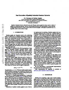
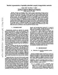
The coupling of network growth with local spatial attachment leads to smallworld networks independent of the dimension of the underlying space. The nodal degree distribution (Fig. 1) and age-degree relationship (Fig. 2) are independent of dimension as in (i). The path length , scales as logN with a coefficient that decreases with dimension (Fig. 3) for fixed average degree. The clustering coefficient C approaches a finite asymptotic value with increasing N (Fig. 4) and this asymptotic value decreases with increasing dimension d of the embedding space. All of our results are very similar for both models, which have different topologies (a unit sphere and a unit ball).

The Sphere Network Model. One natural generalization of embedding nodes on the one-dimensional circumference of a circle is to embed them on the two-dimensional surface of a sphere, or more generally on the d-dimensional surface of a hypersphere (in a space of dimension d 1 1). The case d 5 1 corresponds to the circle network model. However, although it is trivial to arrange N points along the circumference of a circle with uniform spacing, the analogous procedure is less well-defined on higher dimensional surfaces. One way to generalize the arrangement procedure is to consider nodes to act like point charges and to move them to a minimum electrostatic energy equilibrium configuration. The problem of finding the equilibrium configuration of point charges on the surface of a sphere dates back to 1904, when J. J. Thomson introduced his model of the atom, and the problem of obtaining such an equilibrium is sometimes referred to as the ‘‘Thomson problem’’24. A related ‘‘generalized Thomson problem’’ assumes that the force between ‘‘charges’’ is proportional to r2a, where r is the spatial distance between charges, with a not necessarily equal to the Coulomb value, a 5 d25. In order to facilitate comparisons with our second model below, we use the value a 5 d 2 1 in simulations. Using the generalized Thomson problem as a guide, we develop a generalization of the circle network model, which we call the Sphere Network Model, as follows. We model the nodes as point charges confined to a unit spherical surface of dimension d. We successively add a new node onto the surface at random with uniform probability density per unit area and then add links to connect it to its m nearest neighbors in

Degree distribution. The degree distribution H(k) is the probability that a randomly selected node has k network connections. For large N, the degree distribution of the circle network model approaches   1 m k{m H ðkÞ~ ð1Þ mz1 mz1 for k $ m, and H(k) 5 0 for k , m6. Since the number of new links added each time a new node is added is m, Eq. (1) yields the result that the average node degree Ækæ is 2m, satisfying the criterion (i) for the small-world property. Characteristic path length. In the circle network model, simulation results show that , , logN, satisfying criterion (ii). This may be explained intuitively by noting that as new nodes are added, they push apart the older connected nodes, increasing the spatial distance traversed by older edges. These older links dramatically decrease the shortest path length between any given pair of nodes.

SCIENTIFIC REPORTS | 4 : 7047 | DOI: 10.1038/srep07047

Figure 1 | The logarithm of the degree distribution, log(H (k)), versus degree k, for the sphere network model (blue markers) and the plum pudding model (red markers), using N 5 104 and m 5 4. Data are shown for d 5 1 (circles), d 5 2 (triangles), d 5 3 (squares), and d 5 4 (inverted triangles). Since all four cases have nearly identical results, an arbitrary linear offset has been used to separate data for visualization. Error bars are shown when they exceed the point size. Solid black lines correspond to the theoretical prediction of Eq. (1). 2

www.nature.com/scientificreports

Figure 2 | The mean degree kðy,N Þ of a node of age y in a network with N nodes on semilogarithmic axes. Data are shown for the sphere network model (blue) and plum pudding model (red), both with d 5 2, m 5 4, and N 5 104. Errors are smaller than the point size. The solid black line is the theoretical prediction given by Eq. (6). terms of spatial distance. Next we relax the node positions to minimize the potential energy of the configuration using a gradient descent procedure, dx i ~P½F i , dt F i~

X x i {x j  d ,   j=i x i {x j

ð2Þ

ð3Þ

where xi is the (d 1 1)-dimensional position vector of node i, jxij 5 1 for all i, and P [?] denotes projection onto the d-dimensional surface of the sphere. We note that, as new nodes are added, this procedure tends to yield a local energy minimum, as opposed to the global minimum (but for some applications, such as modeling biological network growth, the identification of local rather global minima might be viewed as more appropriate). Note that, for large N, the repulsive interaction ensures that the points are distributed approximately uniformly on the surface of the sphere. The Plum Pudding Network Model. The sphere network model described above has the topological feature that the spatial embedding region does not have any boundary, which allows us to find a nearly-uniform distribution of nodes by imagining them to be identical charges with repulsive interactions. We have also tested another model with a different topology having a boundary and using a different mechanism to encourage uniform distribution of nodes. We call this second model the Plum Pudding Network Model after Thomson’s famous model of the atom24. We again model our nodes as a collection of negative point charges in d dimensions. The growth procedure is similar to the previous models; we place new nodes

Figure 3 | The characteristic graph path length (,) versus network size N on semilogarithmic axes for the sphere model (blue markers) and the plum pudding model (red markers). The path length shows the desired scaling, , , logN. Results are shown for d 5 1 (circles), 2 (triangles), 3 (squares), and 4 (inverted triangles), all using m 5 4. Errors are smaller than the point size. In general, the average shortest path is shorter for higher dimensions d in both models. SCIENTIFIC REPORTS | 4 : 7047 | DOI: 10.1038/srep07047

Figure 4 | Clustering coefficient C versus network size N for the sphere network model (blue markers) and plum pudding model (red markers), both with m 5 4. Results are shown for d 5 1 (circles), 2 (triangles), 3 (squares), and 4 (inverted triangles). Errors are smaller than the point size. Horizontal lines are drawn through the last data point in each series. randomly in our volume and connect them to their m nearest neighbors, where here we define nearest to be the spatial distance between the nodes. Now, however, we regard the nodes as free to move in a unit radius, d-dimensional ball. (For d 5 1, the unit ball is the interval 21 # x # 1; for d 5 2, it is the region enclosed by the unit circle.) We assume that the ball contains a uniform background positive charge density such that the total background charge in the sphere is equal and opposite to that of the N network nodes. As in the sphere model, after adding a node with uniform probability density within the unit d-dimensional ball, we relax the charge configuration to a local energy minimum. Here, the relaxation is described by dx i ~F i {N x i dt

ð4Þ

where xi is a d-dimensional position vector with respect to the center of the ball, Fi is as in Eq. (3), and the term Nxi is due to the positive charge density. Note that, in order to apply Gauss’s law for the background charge, we have assumed a force law proportional to r2(d21). When N is large, the nodes will be approximately uniformly distributed in the ball in order to cancel the uniform positive background charge. Although any repulsive force law can, in principle, be used for the sphere model, we chose to use the same force law for the sphere model in order to facilitate comparisons of the results between the two models. In what follows, we will compare cases of the sphere model and plum pudding model for which the dimension d of the space occupied by the nodes is the same, and we keep a 5 d 2 1 the same for both cases.

Results Degree Distribution. The distribution of node degrees can be derived analytically, does not depend on dimension, and is the same for the sphere and plum pudding models. This can be derived from the fact that, for large N, the probability that a newly added node will form an edge to any particular existing node is m/N for all nodes. This is because existing nodes are distributed approximately uniformly, and new nodes are placed randomly according to a uniform probability distribution. Here we show that for each considered model, we produce the same master equation governing the evolution of the degree distribution as that found for the circle model6. This master equation is not specific to the spatial structure of the network and appears, in various forms, in other network models, such as the Deterministic Uniform Random Tree of Ref. 26. ^ ðk,N Þ to be the number of nodes with degree k at We define G growth step N (i.e., when the system has N nodes). When a node is added to the network it is initially connected to its m nearest neighbors, so upon creation, k 5 m for each node, meaning that ^ ðk,N Þ~0 for k , m. Since each existing node is equally likely to G be chosen to be connected to the new node, there is an m/N probability that any given node will have its degree incremented by 1. ^ ðk,N Þ over all possible random node placements, we Averaging G obtain a master equation for the evolution of G(k, N), the average ^ ðk,N Þ over all possible randomly grown networks, of G 3

www.nature.com/scientificreports m Gðk,N Þ N m z Gðk{1,N Þzdkm , N

Gðk,Nz1Þ~Gðk,N Þ{

ð5Þ

where dkm is the Kronecker delta function. The first term on the right is the expected number of nodes with degree k at growth step N. The second term is the expected number of nodes with degree k at growth step N that are promoted to degree k 1 1. The third term is the expected number of nodes with degree k 2 1 at growth step N that are promoted to degree k. The last term on the right is the new node with degree m. It was shown by Ozik et al.6 that this master equation leads to an exponentially decaying degree distribution with an asymptotically N invariant form H(k) 5 limNR‘ G(k, N)/N given by Eq. (1) for k $ m and H(k) 5 0 for k , m. Interestingly, this degree distribution comes only from the growth process and the uniform probability of attaching new links to existing nodes. As seen in Fig. 1, for m 5 4, N 5 104, with d 5 1, 2, 3, or 4, Eq. (1) is well satisfied by numerical simulations of both models. Intuitively, we expect that older nodes in each model will accumulate more edges and become network hubs. The relationship between degree and age is also straightforward to investigate in this model. Here, we reproduce an expression for the expected degree kðy,N Þ of a node that has existed for y growth steps, given that the network size is N (y , N)27. Each node connects to its m nearest neighbors upon creation, and the probability of incrementing the degree of the node is m/N when the size of the network is N. Thus we obtain kðy,N Þ~mzm

N X

1 n n~N{yz1

  N 1 :