Spatially Fixed and Moving Virtual Sensing Methods for Active Noise

Spatially Fixed and Moving Virtual Sensing Methods for Active Noise Control

Danielle J. Moreau

School of Mechanical Engineering The University of Adelaide South Australia 5005 Australia

A thesis submitted in fulfillment of the requirements for the degree of Ph.D. in Mechanical Engineering on 11 December 2009. Qualified on 12 February 2010.

Chapter 1 Introduction Noise is increasingly becoming recognised as a serious environmental problem and health hazard (World Health Organization, 2001). Human exposure to sustained levels of noise has adverse health effects ranging from nervousness and stress to high blood pressure and loss of hearing. Noise exposure can also increase human error due to worker fatigue and loss of concentration, and increase safety risk through the masking of audible alarms (World Health Organization, 1995). To reduce these health and behavioral effects, strict regulations stating the allowable level of noise at certain times of the day and during certain activities have been introduced. Such regulations have commanded the need for a means of minimising unwanted noise disturbances. Traditionally, passive techniques such as enclosures, barriers and silencers have been used to minimise unwanted noise disturbances. While these devices do generate high attenuation over a broad frequency range, they are less effective at low frequencies and are relatively large in terms of size and cost (Hansen and Synder, 1997). As an alternative to passive methods, active noise control has shown potential in minimising low frequency acoustic disturbances. Active noise control involves the use of one or more secondary sound sources to cancel the primary disturbance, based on the principle of superposition in which antinoise of equal amplitude but opposite phase is combined with the primary noise to cancel both disturbances. Active noise control systems generally consist of a controller which generates a control signal to drive an actuator, usually a loudspeaker, to minimise the sound field sensed by a number of microphones (Kuo and Morgan, 1996). Active noise control has seen rapid recent development due to its potential benefits in size, weight, volume and cost. Currently, active noise control systems are

1

Chapter 1. Introduction

being developed for the attenuation of transportation and automotive vehicle noise, appliance noise such as that produced by air conditioning ducts and refrigerators, and for use in industrial equipment such as fans and pumps (Kuo and Morgan, 1996). Early research in active noise control focused on achieving global control in which the entire sound field is attenuated by minimising the potential energy in an enclosure. However, the level of attenuation achieved with global noise control strategies, especially in modally dense enclosures, is not always sufficient in practical applications (Nelson and Elliott, 1992). As an alternative, local noise control was investigated in which a zone of quiet is generated at the error sensor. While achieving significant attenuation at the error sensor location, local noise control is not without its problems, chiefly that the zone of quiet is generally small and impractically sized. It may be inconvenient to place the error sensor at the desired location of attenuation, such as near an observer’s ear, preventing the small zone of quiet from being centered there. Additionally, large pressure gradients in the vicinity of the error sensor result in significant changes in the perceived sound pressure level as the observer moves around within the zone of quiet. Also of concern is that the sound pressure levels outside the zone of quiet with the active noise control system present are likely to be higher than the original disturbance alone. To overcome the problems encountered in local active noise control systems, virtual acoustic sensors have been developed to shift the zone of quiet away from the physical sensor position to a spatially fixed desired location. A number of virtual sensing algorithms have been developed in the past and these algorithms estimate the sound pressure at the desired location of attenuation, referred to as the virtual location, using the error signal from a remotely located physical sensor (Elliott and David, 1992, Cazzolato, 1999, Roure and Albarrazin, 1999, Cazzolato, 2002, Petersen et al., 2008). This estimate of the sound pressure at the virtual location is then minimised with the active noise control system to generate a zone of quiet at the desired location of attenuation. While virtual sensing algorithms have made it possible to shift the zone of quiet away from the physical error sensor to a desired location of attenuation, in many practical applications this desired location is not spatially fixed. This occurs for example, when a virtual sensor is located at the ear of a seated observer and the observer then moves their head, thereby moving the virtual location. To account for a virtual location that is moving through the sound field, a number of moving virtual sensing algorithms have been developed (Petersen et al., 2006, Petersen, 2007, Petersen et al., 2007). These algorithms have been used to estimate the sound 2

1.1. Literature review

pressure at a moving virtual location using the error signal from a remotely located spatially fixed physical microphone. Minimising the estimate of the sound pressure at the moving virtual location with the active noise control system creates a zone of quiet that tracks the desired location of attenuation as it moves through the sound field. The research presented in this thesis aims to improve and extend the spatially fixed and moving virtual sensing algorithms developed for active noise control thus far and hence increase the scope and application of local active noise control systems. To achieve this research aim, a number of novel spatially fixed and moving virtual sensing algorithms are presented for local active noise control. A full description of the research presented in this thesis to address the general research aim is given in Section 1.2.

1.1

Literature review

This section provides a review of the literature specific to the content of this thesis. In Sections 1.1.1 and 1.1.2, literature investigating global and local active noise control systems is discussed. In Section 1.1.3, a discussion of the research on acoustic energy density control is presented. Finally, Section 1.1.4 presents a review of the literature exploring virtual sensing strategies for active noise control.

1.1.1

Global noise control

Global noise control strategies aim to minimise the sound field at all locations within the acoustic enclosure. An effective measure of the global response of a confined system is the energy stored within it and hence a convenient cost function for evaluating the effect of global noise control is the total acoustic potential energy. Minimising the total acoustic potential energy results in a spatial levelling of the sound field by heavily reducing the amplitudes of the enclosure modes and only slightly reducing the energy between these resonant modes (Nelson and Elliott, 1992). Analysis by Bullmore et al. (1987), Elliott et al. (1987) and Nelson et al. (1987) demonstrated that global control is possible when a lightly damped enclosure is excited close to a natural frequency. The sound field inside the enclosure is dominated by a single modal contribution which can be attenuated without affecting other modes. However, if the enclosure is excited off resonance, a number of residual modes contribute to the response and all of the residual modes cannot be cancelled without exciting 3


others. The physical limitations of an active noise control system in an enclosure are therefore related to the number of modes significantly contributing to the enclosure response at any frequency. A controllability issue also arises when a secondary source is located on a nodal line or surface of an acoustic mode. In this case, the secondary source is unable to drive that mode and it is therefore uncontrollable by the source (Nelson and Elliott, 1992). While minimising the total acoustic potential energy theoretically achieves global reductions in the sound field, a practical control system implementing this cost function would require pressure measurements at all locations within the enclosure. Instead, practical control systems minimise the potential energy estimated by the sum of squared pressures at a number of locations within the enclosure (Nelson and Elliott, 1992). Park and Sommerfeldt (1997) however, demonstrated that achieving global control is difficult with this method due to observability problems which arise when the microphones are located on the nodes of the acoustic modes. Minimising the potential energy estimated by the sum of squared pressures often results in localised zones of attenuation instead of global reductions. Two practical applications which demonstrate the difficulty of obtaining significant global reduction are the global control of engine induced noise in a car cabin and propeller noise in an aircraft passenger cabin. As the sound field inside a car is dominated by harmonics of the engine firing frequency, Elliott et al. (1998) investigated the real-time global control of two harmonics of the engine firing frequency in a car cabin. A feedforward control system was developed using six loudspeakers shared with the in-car entertainment system, eight microphones and a reference signal from the engine ignition circuit. A 4 - 5 dB(A) reduction in the overall A-weighted sound pressure level was achieved in the front and rear seats of the cabin at high engine speeds and 2 - 3 dB(A) of attenuation was achieved at lower engine speeds in the rear of the cabin. The low levels of attenuation achieved at the front and rear cabin seats was attributed to poor coherence between the reference and error sensors. Elliott et al. (1990) implemented an active noise control system in a twin turboprop aircraft cabin to reduce the tonal components of the propeller noise at harmonics of the blade pass frequency (BPF). The active noise control system aimed to attenuate the BPF and its second and third harmonics using 16 loudspeakers and 32 microphones placed around the cabin. A feedforward control approach was employed using a tachometer on one of the propeller engines to generate the reference signals needed to implement feedforward control. Reductions in the overall A-weighted sound pressure level of up to 7 dB(A) were achieved at the microphones 4


at all three harmonics. Johansson et al. (1999) also experimentally investigated the global control of propeller induced noise in an aircraft cabin. Real-time feedforward control of the BPF was investigated in a mock SAAB 340 cabin using 12 loudspeakers to simulate the propeller noise, 12 control microphones and a combination of 5 loudspeakers and 3 small shakers mounted on the fuselage to act as the secondary sources. The mean attenuation in the BPF at the average head height of seated passengers was 18 dB with the two propellers synchronised and only 3 - 6 dB with the propellers unsynchronised. These small reductions in the global sound field demonstrate that it is difficult to achieve perceivable differences in the sound pressure level with global noise control strategies.

1.1.2

Local noise control

As significant global attenuation is difficult to achieve with global noise control strategies, local noise control strategies were instead investigated. Local noise control strategies aim to reduce the sound field at a number of points within the acoustic enclosure to create small localised zones of quiet at the physical error sensors. Olson and May (1953) were the first to suggest the principle of local active noise control through development of an electronic sound absorber. Using feedback control, the electronic sound absorber aimed to attenuate low frequency sound at a physical microphone using a single loudspeaker. At the microphone position, an overall attenuation of 10 - 25 dB was achieved in the broadband disturbance with a frequency range below 200 Hz. Local noise control strategies are suitable for use in complex reactive sound fields unlike global noise control strategies. As discussed in Section 1.1.1, global reductions are possible in enclosures excited at a frequency close to an isolated acoustic resonance (Bullmore et al., 1987, Elliott et al., 1987, Nelson et al., 1987). When the room response is no longer dominated by a single mode but is instead composed of contributions from a number of modes, global noise control strategies are ineffective and local noise control schemes need to be implemented. In fact, it has been shown that global noise control strategies are ineffective at frequencies corresponding to a modal overlap of greater than one, as this indicates that the contribution of the resonant mode is equal to that of the nearby modes (Joseph et al., 1994b). When actively cancelling the sound pressure in a pure tone diffuse sound field in the far-field of the secondary source, the size of the zone of quiet is predictable in

5


a statistical sense. Elliott et al. (1988a) demonstrated that the average sized zone of quiet generated at a microphone by cancelling the measured pressure with a single secondary source is a function of the space-averaged pressure after control and the spatial correlation properties of the sound field. The zone of quiet was found to be defined by a sinc function, with the primary sound pressure level reduced by 10 dB over a sphere of diameter of approximately λ/10, where λ is an acoustic wavelength. Minimising the pressure at a point with a single secondary source was observed to significantly increase the total mean square pressure away from the point of cancellation (Elliott et al., 1988a, Elliott et al., 1988b, Joseph et al., 1994a). In numerical simulations conducted by Elliott et al. (1988a), the total mean square pressure away from the point of cancellation increased by a factor of four with the active noise control system operating. This increase was, however, not repeatable from one simulation to another. The statistical variability in the secondary source strength required to perform pressure cancellation in a pure tone diffuse sound field has also been investigated (Elliott et al., 1988a, Joseph et al., 1994a). The probability density function of the mean square secondary source strength was shown to be an F2,2 distribution (Elliott et al., 1988a, Joseph et al., 1994a). As the mean of this random variable is infinite, the space-averaged squared secondary pressure fails to converge. Physically this is due to the secondary source sometimes being located at a position where it has little effect on the pressure at the sensor location. As a result, the magnitude of the secondary transfer function will be small and the secondary source strength correspondingly large. This explains the lack of repeatability between ensemble averages used to determine the average sized zone of quiet in numerical simulations. Joseph et al. (1994a) investigated the cancellation of sound pressure at a point in the near-field of a secondary source in a pure tone diffuse sound field. In comparison to far-field cancellation, the size of the zone of quiet in the near-field is deterministically defined by the near-field characteristics of the secondary source. Also, the secondary source strength is significantly reduced compared to far-field cancellation and is not dependent on the statistical properties of the sound field (Joseph et al., 1994a). In the near-field of the secondary source (2πr0 λ), the 10 dB zone of quiet has a diameter equivalent to 0.6r0 , where r0 is the radial distance between the source and the cancellation point. The zone of quiet generated in the near-field of the secondary source therefore increases in size as the distance between the cancellation point and the secondary source, r0 , increases. Specifically, if the distance between the secondary source and the cancellation point is greater than λ/5, the size of the 6


10 dB zone of quiet approximates λ/10, as is the case for far-field cancellation. Rafaely (2001) extended previous research (Elliott et al., 1988a, Joseph et al., 1994a) to theoretically analyse the spatial extent of the localised zones of quiet generated in a broadband diffuse sound field. Using a previously derived expression for the correlation coefficient applicable to both broadband and pure tone diffuse sound fields (Rafaely, 2000), expressions for the zone of quiet generated in both the nearfield and far-field of the secondary source were derived. Numerical simulations were also performed to investigate the size of the zone of quiet generated in a number of tonal and broadband diffuse sound fields of different frequencies. Results demonstrated that the size of the zone of quiet generated in a broadband diffuse sound field is similar to that generated in a pure tone diffuse sound field at the centre frequency of the broadband frequency range. David and Elliott (1994) conducted numerical simulations to investigate the size of the zone of quiet generated at a microphone both on- and off-axis of a secondary source. The performance of the local active noise control system in uniform and diffuse sound fields was investigated with the secondary sound source being modelled as a piston in an infinite baffle. In a uniform sound field at low frequencies, the zone of quiet is a shell shape whose size is independent of frequency. At higher frequencies, the zone of quiet decreases in size until it becomes a sphere with diameter λ/10. This is the same sized zone of quiet as that derived by Elliott et al. (1988a) for far-field cancellation in a pure tone diffuse sound field. Similiar sized zones of quiet were generated both on- and off-axis of the secondary source up to a frequency of 1 kHz. On-axis of the secondary source, in both uniform and diffuse sound fields, the 10 dB zone of quiet increased in size as the distance from the cancellation point to the secondary source increased up to the limiting distance of λ/10. 1.1.2.1

Applications of local noise control

Local active noise control systems have been successfully implemented in the headrest of a passenger seat. Rafaely et al. (1997) and Rafaely and Elliott (1999) investigated a local active headrest system implementing a feedback controller. The controller was designed using Internal Model Control (IMC) and a combination of H2 and H∞ methods. The system included a single secondary loudspeaker mounted in the headrest and a physical microphone placed 2 cm from the loudspeaker and 10 cm from the ear of a manikin, as shown in Fig. 1.1. The controller had the performance objective of minimising the variance of the microphone output while

7


NOTE: This figure is included on page 8 of the print copy of the thesis held in the University of Adelaide Library.

Figure 1.1: Local active headrest (Rafaely et al., 1997). being subject to robust stability, disturbance enhancement limits and limits on the power to the actuators. The cost function and system constraints were H2 and H∞ functions of the control filter coefficients. Using discretised frequency response functions in the cost function and constraints, the frequency control filter coefficients were then solved using convex optimisation. The frequency response functions were measured in an experimental setup and used in off-line analysis of the controller. An overall attenuation of 15.7 dB was obtained in the broadband disturbance at the physical microphone, over a 100 - 400 Hz frequency range. Despite good attenuation at the physical microphone, only 3.7 dB of attenuation was achieved at the ear of the manikin. Brothanek and Jiricek (2002) investigated the performance of a two-channel active headrest system in a broadband free field with a 100 - 500 Hz frequency range. The headrest contained two secondary loudspeakers and two physical microphones located 5 cm from the loudspeakers and 7 cm from a manikin’s ears. The measured pressures at the two microphones were minimised by a feedforward controller implementing the Filtered-x LMS (Fx-LMS) algorithm. An attenuation of 15 - 20 dB was achieved in the broadband disturbance at the physical microphones, however, only 10 dB of attenuation was achieved at the manikin’s ear. A double input - quadruple output local active headrest was developed by Pawelczyk (2003a), using feedback control. The controller was designed to minimise a 250 Hz tonal disturbance at two microphones located 15 cm from the manikin’s ears, using four loudspeakers. While 32 dB of attenuation was achieved at the physical microphones with the double input - quadruple output active headrest, only 8


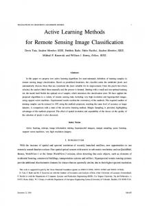
18 dB of attenuation reached the manikin’s ears. In comparison, a double input double output local active headrest, which minimises the pressures at two physical microphones with two loudspeakers, achieved 30 dB of attenuation at the physical microphones and only 11 dB of attenuation at the manikin’s ears. As the performance of the local headrest will be influenced by the presence of a seated passenger’s head, Garcia-Bonito and Elliott (1995a) and Garcia-Bonito et al. (1997a) theoretically investigated the effect of a diffracting sphere on the size of the zone of quiet in a diffuse sound field. In numerical simulations, the presence of the diffracting sphere was seen to increase the size of the zone of quiet as it extends towards the reflective surface. This size increase is due to an imposed zero normal pressure gradient on the surface of the sphere. As the sphere approximates a human head, it is expected that a seated passenger in the active headrest would have a beneficial effect on the size of the zone of quiet. In an effort to extend the localised diffuse field zone of quiet to the size of a human head, Zou et al. (2007) developed a virtual sound barrier. A virtual sound barrier is an array of loudspeakers and microphones generating a zone of quiet within the volume bounded by the microphones. Zou et al. (2007) investigated a 16 channel cylindrical virtual sound barrier system whose physical arrangement of control sources and microphones is shown in Fig. 1.2. The loudspeakers are arranged on the two horizontal circular ends of a cylinder with radius, ac , and height, hc , of 1.2 m. The error sensors are similarly arranged on a cylinder with radius, ae , and height, he , of 0.2 m. The performance of the virtual sound barrier was experimentally investigated inside a 4 m × 4 m × 5 m enclosure. A 16 channel feedforward controller implementing the filtered-x LMS algorithm generated the control source strengths using the sum of squared pressures as the desired cost function. Experimental results demonstrated that the level of attenuation achieved within the virtual sound barrier decreased with increasing frequency. A 10 dB zone of quiet with diameter of 0.66λ, or the effective size of a human head, was generated in a pure tone diffuse sound field with frequency below 550 Hz. As the aim of the virtual sound barrier system is to create a zone of quiet around a human head, Zou and Qiu (2008) experimentally investigated the effect of placing a diffracting sphere inside the virtual sound barrier. Using the same experimental setup as previously (Zou et al., 2007), a hollow iron sphere of radius 0.09 m was placed at the centre of the virtual sound barrier to act as the human head. The experimental results demonstrated that the presence of the diffracting sphere has the beneficial effect of smoothing out the pressure attenuation. With the diffracting 9

Chapter 1. Introduction Control sources ac ae hc

he Error sensors

Control sources Figure 1.2: Physical arrangement of control sources and errors sensors to generate a virtual sound barrier (Zou et al., 2007). sphere, the pressure distribution within the virtual sound barrier becomes more uniform in the normal direction to the sphere surface. Kuo (2006) experimentally investigated the active cancellation of non-stationary, intermittent snoring noise at the ear of a bed partner using feedforward control. The experimental setup, shown in Fig. 1.3, consisted of two loudspeakers and two microphones mounted in a headboard surrounding the head of a KEMAR human torso model acting as the bed partner disturbed by the snoring noise. Microphones were also installed in the ear cavity of the KEMAR model to evaluate the performance of the active noise control system at the ear position. The broadband snore disturbance with 100 - 300 Hz frequency range was simulated by a loudspeaker mounted in the headboard of a second twin-sized bed in the same room. A reference microphone mounted in the headboard close to the primary loudspeaker provided the reference signal to the feedforward controller. In real-time experiments, the signals from the two microphones were combined to produce a single error signal and the same control signal was used to drive both secondary sources. With this method, the average attenuation at the microphones was 10 - 20 dB. Only 5 - 10 dB of attenuation was, however, achieved at the left ear of the KEMAR model. Kuo and Gireddy (2007) experimentally investigated the performance of a multi-channel snore active noise control system in which two secondary loudspeakers were used to minimise the broadband snore disturbance at two microphones. Using the same experimental setup as Kuo (2006), an average attenuation of 7 - 12 dB was achieved at the manikin’s right ear and 2 - 5 dB was achieved at the manikin’s left ear when

10



Figure 1.3: Experimental setup of the snore active noise control system (Kuo, 2006).

the two microphones were located in the headboard. This average noise attenuation increased to 18 - 20 dB at both ears when the two microphones were placed close to the head of the KEMAR model. An intrauterine acoustics embedded active noise control system has been developed by Thanigai and Kuo (2007) to reduce noise inside infant incubators in Neonatal Intensive Care Units (NICUs). An example of a mobile infant incubator seen in NICUs is shown in Fig. 1.4. The broadband noise disturbance inside the incubator is generally produced by ventilation or breathing equipment and human activity. The active noise control system, while minimising the unwanted noise disturbance, also introduces intrauterine audio into the incubator to create a more comfortable environment for the infant and to mask any residual noise. The added intrauterine audio consists of a heart beating and the sound of blood and fluid movement. The performance of the intrauterine active noise control system was investigated using experimentally measured data from a model incubator. Microphones were placed at the intended infant’s head position and a secondary loudspeaker was placed outside the incubator behind the infant’s head position. A feedforward controller was developed using a modified version of the Filtered-x Least Mean M-estimate (FxLMM) algorithm with online secondary path modelling. The Fx-LMM algorithm is robust in the presence of impulsive noise that may cause the Fx-LMS algorithm to become unstable. Impulsive noise is common in NICUs and is typically caused

11



Figure 1.4: An infant incubator in a neonatal intensive care unit (Thanigai and Kuo, 2007). by medical equipment such as ventilators and human activity. The intrauterine audio was added to the secondary cancelling noise so that it could be heard by the infant. This audio was also subtracted from the error signal to generate the true error signal used to update the adaptive filter coefficients. An average attenuation of 16 dB was achieved in the broadband disturbance below 1 kHz at the error sensor locations with the intrauterine audio being successfully introduced once the active noise control system had converged.

1.1.3

Acoustic energy density control

An alternative to the traditional pressure squared cost function implemented in many local and global active noise control systems is an acoustic energy density cost function. Acoustic energy density is formed by the sum of acoustic potential energy density and acoustic kinetic energy density, and in practice is calculated using the weighted sum of squared pressure and squared particle velocity. The most common method of estimating the pressure and particle velocity is the two-microphone technique which uses two closely spaced, phase-matched pressure microphones (Fahy, 12


1995). With the two-microphone technique, the pressure is estimated midway between the two microphones and the particle velocity is calculated using a finite difference approximation. Acoustic energy density represents the total energy at a point and has been found to be an effective cost function for both local and global active noise control applications (Sommerfeldt and Nashif, 1994, Sommerfeldt and Parkins, 1994, Kestell, 2000). Minimising an acoustic energy density cost function overcomes the observability problems associated with reducing the squared pressure and outperforms a potential energy density cost function estimated by microphones (Sommerfeldt and Nashif, 1994, Sommerfeldt and Parkins, 1994, Elliott and GarciaBonito, 1995). As acoustic energy density is the sum of the potential and kinetic energy densities, minimising the energy density at a point reduces the sound pressure and particle velocity at that point. Particle velocity is directly proportional to the pressure gradient through Euler’s equation (Nelson and Elliott, 1992) and therefore minimising the pressure and pressure gradient at a point is equivalent to energy density control. Elliott and Garcia-Bonito (1995) investigated the local control of both pressure and pressure gradient in a pure tone diffuse sound field with two secondary sources. Minimising both the pressure and pressure gradient along a single axis produced a far-field zone of quiet over a distance of λ/2, in the direction of pressure gradient measurement. This is considerably larger than the zone of quiet obtained by minimising the pressure alone (in which the 10 dB zone of quiet was limited to λ/10). This size increase can be explained by the fact that the average size of the zone of quiet is a function of the spatial correlation properties of the sound field. The squared sum of the pressure and pressure gradient cross correlation functions extend over a larger region compared to the squared pressure correlation function alone. It should be noted that cancelling the pressure and pressure gradient along a single axis produces a similar sized zone of quiet to that generated by minimising the pressures at two points separated by a maximum distance of 0.25λ. As there is no correlation between the pressure gradients in the three orthogonal directions, minimising the pressure gradient along a single axis will not affect the pressure gradient along the remaining two axes. Controlling the pressure and pressure gradient along a single axis with two secondary sources produces a 10 dB zone of quiet which is cylindrical in form, with size λ/2 in the direction of gradient cancellation and λ/10 in the two remaining orthogonal directions. As expected, cancelling the pressure and pressure gradient along all three orthogonal axes with four secondary sources results in a spherical zone of quiet with diameter of λ/2. 13


Improvement in the overall global attenuation achieved by minimising a potential energy cost function (estimated by the sum of squared pressures) is possible by instead minimising the acoustic energy density in the sound field (Sommerfeldt and Parkins, 1994, Sommerfeldt et al., 1995). This is due to increased observability when sensing the acoustic energy density. If the error sensor is located at a potential energy node in the sound field, the magnitude of the kinetic energy density will approach a maximum. Therefore, as the spatial variance of the acoustic energy density is less than that of potential energy, the observability problems associated with discrete pressure measurements can be overcome with an acoustic energy density cost function (Sommerfeldt and Nashif, 1994). Sommerfeldt and Nashif (1994) developed a control law based on the filtered-x LMS algorithm for controlling the global energy in an acoustic standing wave and also a propagating wave field. In the adaptive algorithm the acoustic pressure and particle velocity were measured using the two-microphone technique which estimates the pressure and particle velocity components using a finite difference approximation. The performance of the adaptive algorithm was investigated in an acoustic duct with single frequency excitation at 200 Hz. Numerical and experimental results confirmed the effectiveness of the energy based control law and demonstrated that acoustic energy density control significantly outperforms pressure control. Sommerfeldt and Nashif (1991, 1992) also numerically and experimentally investigated energy density control in the global attenuation of acoustic duct noise. Controlling the acoustic energy density at a discrete location with a single secondary source was seen to almost achieve the optimal solution of minimising the potential energy and significantly outperformed control with a pressure squared cost function. Park and Sommerfeldt (1997) extended this research to demonstrate that energy density control can be used in the global attenuation of broadband noise disturbances. Numerical simulations performed in a one-dimensional sound field indicated, as previously, that greater global control can be achieved by minimising the acoustic energy density at a point compared to minimising the acoustic pressure. Unlike pressure control, the global attenuation achieved was independent of the error sensor location, demonstrating another advantage of an acoustic energy density cost function. Sommerfeldt and Nashif (1991, 1992, 1994) and Park and Sommerfeldt (1997) all performed numerical simulations using a rigid-walled one-dimensional modal model to investigate acoustic energy density control. Cazzolato et al. (2005b) demonstrated, however, that miscalculation occurs when using this modelling technique and that previous theoretical results may have been adversely affected by numer14


ical noise. Using a travelling wave solution, it was shown that a pressure-release boundary condition is created when the secondary source is located upstream of the two microphones. Complete attenuation of the energy density is therefore possible downstream of the secondary source. Such a result was not achieved in previous research (Sommerfeldt and Nashif, 1991, Sommerfeldt and Nashif, 1992, Sommerfeldt and Nashif, 1994, Park and Sommerfeldt, 1997) because noise is introduced into the model when the numerical precision of the computer program is reached preventing convergence of the modal model to the travelling wave solution. Sommerfeldt et al. (1995) numerically and experimentally compared pressure and acoustic energy density cost functions for global control in a tonal three-dimensional sound field. The experimental configuration consisted of a primary source, a secondary source and an error sensor located in a rectangular enclosure with dimensions of 1.93 m × 1.22 m × 1.54 m. To measure the acoustic energy density, an inexpensive energy density probe was constructed using six Lectret 1207a microphones flush mounted in a wooden sphere. Results of feedforward control once again demonstrated that minimising the acoustic energy density at a single location within the enclosure provides improved global performance compared to minimising the pressure alone. Sommerfeldt (2006) investigated the global attenuation of low frequency engine induced sound in the cab of a Caterpillar Inc. earth-moving vehicle using acoustic energy density control. The aim was to achieve significant attenuation in the third engine tone over the 50 - 110 Hz frequency range throughout the entire operator cab. Two 4” loudspeakers and an 8” subwoofer were mounted in the cab and an energy density sensor was positioned above the operator’s head. The energy density sensor consisted of six pressure microphones mounted in a circular sphere. A feedforward control approach was employed using the engine tachometer signal as the reference signal. In real-time experiments, minimising the acoustic energy density achieved an overall attenuation of 5 - 7 dB(A) in the third engine tone throughout most of the cabin. Miyoshi and Kaneda (1991) experimentally investigated the cancellation of the pressures at two points with three secondary sources in a broadband diffuse sound field with 50 - 400 Hz frequency range. The active noise control system consisted of three noise-control units each of which filtered the signal from a reference microphone to produce the control source strengths to one of three secondary sources. The filters were determined using the Multiple input/output INverse-filtering Theorem (MINT). Experiments were conducted in a room with a volume of 70 m3 and 15


reverberation time of 0.4 s. The three secondary loudspeakers were located on a circle with a 1.2 m radius, centred on the midpoint between the two microphones. The two microphones were separated by a distance of λ/4, where λ is the wavelength of the centre frequency of the broadband frequency range. Attenuations of 30 dB were achieved at the two cancellation points with 14.5 dB of attenuation being achieved in the region between them. The 6 dB zone of quiet centred on the midpoint between the two microphones was an ellipse with longest diameter λ/2 and shortest diameter λ/8. 1.1.3.1

Errors in the measurement of acoustic energy density

Despite energy density sensors being effective in both local and global active noise control applications (Sommerfeldt and Nashif, 1994, Sommerfeldt and Parkins, 1994, Kestell, 2000), the measurement of acoustic energy density is subject to errors. Such errors include those associated with the calculation of pressure and particle velocity when using the two-microphone technique, imperfections in the sensor transducers, sensitivity and phase mismatch between microphone elements, diffraction, interference and environmental effects (Fahy, 1995). The three distinct sources of error attributed to the measurement of acoustic energy density using the two-microphone technique are inherent errors, diffraction and interference effects, and instrumentation errors. Cazzolato and Hansen (2000b) derived expressions for the effects of these errors on the performance of one-dimensional energy density sensors with 2or 3-microphone arrangements. The inherent errors due to the finite approximation of pressure and particle velocity limit the high frequency range of the energy density sensor and the maximum sensor size. As the 3-microphone arrangement directly measures the pressure at the centre microphone, inherent errors are purely due to errors in the velocity approximation. Instrumentation errors such as phase and sensitivity mismatches between the microphone elements were found to define the lower frequency limit and the minimum sensor size. In an extension to previous work, Cazzolato and Hansen (2000a) investigated various physical configurations of three-dimensional energy density sensors and performed a three-dimensional error analysis to determine the most suitable error sensor design. Four three-dimensional sensor configurations were investigated: the conventional 6-microphone configuration; a 7-microphone configuration in which an additional microphone is located at the geometric centre of the 6-microphone sensor; and two 4-microphone configurations in which the pressure is measured at the central mi-

16


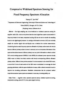
crophone alone or is the mean of the pressure sensed by all four microphones. These four sensor configurations are shown in Fig. 1.5. Results of analysis conducted in a plane progressive wave and a reactive sound field demonstrated that acoustic energy density can be adequately measured using only a 4-microphone sensor instead of the conventional 6-microphone sensor. In comparison to the errors recorded using onedimensional sensors, the errors for the three-dimensional sensors were three times larger than the equivalent one-dimensional sensors at the low frequency limit. However, at the high frequency limit, the errors for the three-dimensional sensors were less than those for the one-dimensional sensors. The 4-microphone sensor that measures the pressure directly at the central microphone is the simplest of all designs and was found to be the best for free field use. In reactive conditions, the 7-microphone sensor was found to measure the acoustic energy density most accurately. Parkins et al. (2000) investigated bias errors in the estimate of the potential, kinetic and acoustic energy density when using a single-axis two-microphone sensor and a single-axis spherical sensor comprised of two microphones flush mounted in a sphere. The main advantage of the spherical sensor over the conventional twomicrophone sensor is that the diffraction effects allow the effective sensor size to be reduced by a factor of 3/2. The bias error equations for the single-axis sensors were derived for a one-dimensional standing wave field with and without sensitivity and phase mismatch introduced between microphone elements. The bias errors were investigated for three cases of reflection coefficient: R=±0.97, corresponding to the sensor being located at a pressure maximum or minimum; and R=0, corresponding to plane wave propagation. The bias errors in the potential and kinetic energy density estimates were found to be equal for all values of reflection coefficient. For matched microphones, the bias errors were found to be small and the effect of spherical scattering on the spherical sensor reduced the bias errors considerably. However, when phase and sensitivity mismatch were introduced between microphone elements, the bias errors were significantly increased and spherical scattering no longer influenced these errors. Parkins et al. (2000) also investigated bias errors in the estimate of the potential, kinetic and total acoustic energy density when using a three-axis spherical energy density sensor in a three-dimensional sound field. The three-axis spherical sensor, shown in Fig. 1.6, consisted of six microphones oriented along the orthogonal axes and flush mounted in a sphere. Results of numerical simulations to determine the potential, kinetic and energy density bias errors were consistent with those for the single-axis spherical sensor. Overall, the error magnitude in the total energy density estimate for mismatched microphones was less than 1 dB. A 17


z

y

x

Figure 1.5: Energy density sensor in 4-microphone and 6- or 7-microphone configurations (Cazzolato and Hansen, 2000a). three-axis spherical sensor was constructed and then tested in a three-dimensional rectangular enclosure with a white noise disturbance to experimentally verify numerical results. The spherical sensor consisted of a 2” diameter wooden ball with three electret microphone pairs mounted along the orthogonal axes. A B&K 14 ” microphone pair was used as a two-microphone sensor for comparison. With the two-microphone sensor, the total acoustic energy density was calculated using the spectral quantities measured with a two-channel spectrum analyser and a derived energy density spectral density equation. The total energy density estimate using the spherical sensor was found to be within ±1.75 dB of that estimated with the two-microphone sensor in the frequency range of 110 - 400 Hz. Differences in the energy density estimated with the two sensor arrangements were attributed to sensitivity and phase mismatch, diffraction due to the sphere and experimental error. It was later shown by Cazzolato and Ghan (2005) however, that the energy density spectral density equation derived by Parkins et al. (2000) and used in experiments to estimate the energy density with the two-microphone sensor was incorrect by a factor of 2. Ghan et al. (2003) derived one-dimensional expressions for frequency domain time-averaged energy density spectral density estimates using the two-microphone method. Direct calculation in the frequency domain removes the need for the additional hardware required when performing analysis in the time domain. Cazzolato and Ghan (2005) then extended the concepts previously introduced by Ghan et al. (2003) to estimate the three-dimensional acoustic energy density using spectral 18


Figure 1.6: Three-axis spherical acoustic energy density sensor (Parkins et al., 2000).

methods. Analytical expressions for the single-sided time-averaged energy density spectral density estimate were derived for several three-dimensional energy density sensor configurations including the 4-microphone sensor in cubic and tetrahedral formation, the 6-microphone sensor and the 7-microphone sensor. The derived expressions use only the auto- and cross-spectral densities between closely spaced microphones allowing evaluation of the energy density spectral density to be performed using only data from a two-channel spectrum analyser. All derived expressions were verified numerically by comparison to traditional time domain estimates of acoustic energy density. Ghan et al. (2004) also analysed the normalised random errors associated with the estimation of the time averaged acoustic energy density spectral density estimate in the frequency domain. It was shown that the normalised error depends heavily on the number of averages used to produce the spectral density estimates. A recent study by Pascal et al. (2008), however, stated that the statistical errors in the frequency domain estimate of the acoustic energy density are largely determined by the nature of the sound field, in particular, the coherence between microphone elements. Approximate expressions for the frequency domain estimate of the acoustic energy density were derived by Pascal and Li (2008). The frequency domain acoustic energy density expressions were derived for two 4-microphone probes in cubic and tetrahedral arrangement as well as two 5-microphone and two 6-microphone probe arrangements. A finite sum approximation was used to estimate the pressure and the two-microphone technique to estimate a component of the pressure gradient. As previously, these expressions require only the auto- and cross-spectral densities between closely spaced microphones. The errors associated with the finite difference 19


and finite sum approximations at high frequencies were analysed in a plane wave sound field. No difference was observed between the two types of 4-microphone tetrahedral probe arrangements in the error analysis. Although the derived acoustic energy density frequency domain expressions for the two probe configurations were different, the orientation of the probes had no affect on the magnitude of the errors. The addition of a fifth microphone resulting in the 5-microphone probe arrangements, demonstrated limited improvement by increasing the high frequency limit by 13%. The high frequency limit is defined based on a fixed maximum error criterion and is the frequency at which this maximum allowable error occurs. In this case, the maximum allowable uncertainty was 5%. The 6-microphone probe arrangements were seen to improve the energy density estimate only if the pressure was estimated using the average of all microphone elements. The errors associated with energy density sensors using the two-microphone technique have commanded the need for alternative methods of measuring the acoustic energy density. One such alternative is to use sensors that directly measure the particle velocity rather than using a finite difference approximation. However, velocity microphones have been known to have a poor frequency response and to lack robustness and dynamic range (Cazzolato et al., 2005a). As an alternative to the two-microphone technique, the μflown sound intensity probe incorporating MicroElectro-Mechanical-Systems (MEMS) technology was developed (de Bree, 1998, de Bree et al., 1999). The μflown sound intensity probe directly measures velocity but avoids the problems associated with conventional velocity sensors. The velocity sensors do, however, exhibit a complex sensitivity curve and the intensity probe is expensive, making it unsuitable for use in many active noise control applications. Recently, Cazzolato et al. (2005a) reported development of the PHONE-OR optical sensor capable of measuring both sound intensity and acoustic energy density along all three orthogonal axes. The device consists of an omni-directional pressure microphone and three orthogonally mounted pressure gradient microphones to measure the pressure and particle velocity in all three orthogonal directions. The PHONEOR Fibre Optical Microphones (FOM) were developed using MEMS technology and as such, the problems affecting conventional energy density sensors and velocity microphones are avoided. Other advantages of the PHONE-OR optical sensor include a high bandwidth, low self noise, a flat frequency response over the dynamic range and smaller size compared to conventional energy density probes. Lockwood and Jones (2006) reported recent development of an acoustic vector sensor (AVS) for use in air. Commonly used in underwater acoustic sensing applications, AVS 20


are used to directly measure the pressure and particle velocity in three orthogonal directions simultaneously. The sensor consists of an omnidirectional microphone (commercially available Knowles EK-3132) and three orthogonally orientated gradient microphones (commercially available Knowles NR-3158) collocated on a thin rod. While being developed for use with beamforming algorithms, these sensors are capable of measuring sound intensity and acoustic energy density.

1.1.4

Virtual sensing

It has been shown that the zone of quiet generated at the physical error sensor using traditional local active noise control systems is limited in size. Also, the sound pressure levels outside the zone of quiet are likely to be higher than the original disturbance alone with the active noise control system present. This is illustrated in Fig. 1.7 (a) where the zone of quiet located at the physical error sensor is too small to extend to the observer’s ear and the observer in fact experiences an increase in the sound pressure level with the active noise control system operating. A virtual acoustic sensor overcomes this by shifting the zone of quiet to a desired location that is remote from the physical sensor. This is shown in Fig. 1.7 (b) where the zone of quiet is shifted from the physical sensor to a virtual sensor located at the observer’s ear. Using the physical error signal, the control signal and knowledge of the system, a virtual sensing algorithm is used to estimate the pressure at a fixed virtual location. Instead of minimising the physical error signal, the estimated pressure is minimised with the active noise control system to generate a zone of quiet at the virtual location. Elliott and David (1992) first introduced the concept of virtual sensing for active noise control through development of the virtual microphone arrangement. A number of virtual sensing algorithms have since been developed to estimate the virtual quantities including the remote microphone technique (Roure and Albarrazin, 1999), the forward difference prediction technique (Cazzolato, 1999), the adaptive LMS virtual microphone technique (Cazzolato, 2002) and the Kalman filtering virtual sensing method (Petersen et al., 2008). A discussion of these virtual sensing algorithms is presented in the following sections. It is worth noting that virtual sensing is essentially the reconstruction of unknown data or that which is difficult to obtain from available measurements (Goodwin, 1999). As such, the scope of virtual sensing extends far beyond that of active noise control applications. Virtual sensors have been implemented in a number of technological systems including radar, biomedical, industrial, communications and

21

Chapter 1. Introduction Virtual sensor Physical sensor

Physical sensor Primary noise

Primary noise

NOTE: This figure is included on page 22 Controlled of the print copy of the thesis held in noise Controlled noise the University of Adelaide Library. (b)

(a)

Figure 1.7: Comparison of local active noise control at (a) a physical sensor; and (b) a virtual sensor (Kestell, 2000). control (Goodwin, 1999). Specific industrial application of virtual sensors includes temperature estimation for shape control applications, process quality attribute estimation in a food extruder, tracking near geostationary satellites for communication purposes and thickness estimation in rolling mills (Albertos and Goodwin, 2002). Kammer (1997) demonstrated that virtual sensors can be used in structural response estimation. Using a transformation matrix and vibration data from accelerometers placed at discrete locations on a structure, the structural response at inaccessible locations can be calculated. The transformation matrix is estimated in a preliminary identification stage using the impulse response function obtained from a vibration test of the structure. 1.1.4.1

The virtual microphone arrangement

The virtual microphone arrangement proposed by Elliott and David (1992) was the first virtual sensing algorithm developed for active noise control. This virtual sensing algorithm uses the assumption of equal primary sound pressure at the physical and virtual locations and requires a preliminary identification stage in which models of the secondary transfer functions are estimated. Virtual sensing algorithms similar to the virtual microphone arrangement have also been proposed by Kuo et al. (2003) and Pawelczyk (2003c, 2004b, 2005). The performance of the virtual microphone arrangement has been thoroughly investigated in both tonal and broadband sound fields (Garcia-Bonito and Elliott, 1995b, Garcia-Bonito et al., 1996, Matsuoka et al., 1996, Garcia-Bonito et al., 1997b, Garcia-Bonito et al., 1997c, Horihata et al., 1997, Rafaely et al., 1997, Rafaely et al.,

22


1999, Holmberg et al., 2002, Pawelczyk, 2003a, Pawelczyk, 2003b, Pawelczyk, 2003c, Pawelczyk, 2004a, Pawelczyk, 2004b, Pawelczyk, 2005, Diaz et al., 2006, Pawelczyk, 2006). Analysis of the virtual microphone arrangement in a pure tone diffuse sound field by Garcia-Bonito et al. (1996, 1997b) demonstrated that at low frequencies, the zone of quiet generated at a virtual microphone is comparable to that achieved by directly minimising the measured pressure at the virtual location. However, at higher frequencies, above 500 Hz, the 10 dB zone of quiet is substantially smaller when using a virtual microphone compared to a physical microphone at the same location. This is due to the assumption of equal primary sound pressure at the physical and virtual microphone locations being invalid at high frequencies. The performance of a local active headrest system implementing the virtual microphone arrangement has been investigated by a number of authors (Garcia-Bonito et al., 1996, Garcia-Bonito et al., 1997b, Rafaely et al., 1997, Rafaely et al., 1999, Holmberg et al., 2002, Pawelczyk, 2003b, Pawelczyk, 2003c, Pawelczyk, 2004b). Garcia-Bonito et al. (1996, 1997b) experimentally investigated the performance of a two-channel local active headrest system in minimising a tonal disturbance at virtual microphones located 2 cm from the ears of a manikin and 10 cm from the physical microphones. At low frequencies, when the primary acoustic field at the physical and virtual microphones is similar, good attenuation is achieved at the virtual location. Below 500 Hz, combining this virtual sensing algorithm with the Fx-LMS algorithm extends the 10 dB zone of quiet generated at the virtual microphone approximately 8 cm forward by 10 cm side to side. At higher frequencies, however, the assumption relating to the similarity of the primary field at the physical and virtual microphones is no longer valid and limited attenuation is achieved at the virtual location. The performance of a local active headrest system in attenuating a broadband disturbance with a 100 - 400 Hz frequency range was investigated by Rafaely et al. (1997, 1999) using feedback control. A single input-single output feedback controller was designed using a mixed H2 /H∞ method and IMC. The controller performance was analysed off-line at a virtual microphone located at a manikin’s ear, 10 cm from the physical microphone, using experimentally measured frequency response functions. An overall attenuation of 9.5 dB was obtained at the virtual microphone location with the virtual microphone arrangement. This is compared to 19 dB of attenuation being obtained at the physical microphone by directly minimising the measured pressure signal. Although significant attenuation is achieved at the physical microphone with this method, only 3.7 dB of attenuation is achieved at the ear of the manikin. Differences in the attenuation achieved by minimising the physical 23


and virtual microphone signals were partly attributed to the physical microphone being significantly closer to the secondary loudspeaker than the virtual microphone. This results in a longer delay in the virtual plant, which has a negative effect on the performance of the feedback control system. Pawelczyk (2003c) developed a double input - double output feedback controller for a local active headrest system. An algorithm using the same assumption as the virtual microphone arrangement, namely that the primary disturbance at the physical and virtual microphones is equal, was used to estimate the disturbance at two virtual microphones located at the manikin’s ears. The two physical microphones were located in the headrest below two secondary loudspeakers, a distance of 15 cm away from the manikin’s ears. Controlling a 250 Hz tonal disturbance achieved attenuations of 18 dB at the virtual locations. In comparison to classical algorithms, attenuations of 30 dB were achieved at the physical microphones by directly minimising the measured disturbance. The greatest attenuation is achieved at the physical microphones with this method and only 10 dB of attenuation reaches the manikin’s ears. In an extension, Pawelczyk (2003b) developed a double input - quadruple output feedback controller for an active headrest. This local active headrest system aims to minimise the tonal disturbance at two virtual microphones located at the manikin’s ears with four secondary sources. In experiments, attenuations of 20 dB were achieved at the manikin’s ears and the size of the zone of quiet was seen to increase compared to that achieved with the double input - double output feedback controller. Directly minimising the physical error signals achieved 32 dB of attenuation at the two physical microphone locations and 18 dB of attenuation at the manikin’s ears, indicating that the zone of quiet has been enlarged with this controller. Pawelczyk (2004b, 2005) proposed another virtual sensing algorithm similar to the virtual microphone arrangement for a local active headrest system implementing a feedback controller. In a preliminary identification stage, the feedback controller is tuned to minimise the signals measured at microphones temporarily located at the virtual locations. A transfer function modelling the physical error signals that exist when the controller has converged is measured during this preliminary identification stage. The difference between the signals computed with this transfer function and the actual physical microphone signals is minimised with the controller during real-time control. This version of the virtual microphone arrangement has been implemented in a double input - double output active headrest system, with the virtual microphones located 6.5 cm from the physical microphones. In a tonal sound field 24


at 250 Hz, attenuations of 30 dB were achieved at the virtual locations. In a broadband sound field with a dominating frequency of 330 Hz, the attenuation achieved at the virtual microphones was reduced to 4 dB. Pawelczyk (2006) also developed a feedback controller for an active headrest system implementing this modified version of the virtual microphone arrangement using a factorisation approach. In numerical simulations, an attenuation of 8.6 dB was achieved at a virtual microphone located at an observer’s ear, over a 100 - 400 Hz frequency range. Holmberg et al. (2002) developed a low complexity, robust feedback controller for a single-channel active headrest system implementing the virtual microphone arrangement. The controller was designed to attenuate a 140 Hz tonal disturbance at a virtual microphone located 8 cm from the physical microphone and 12 cm from the secondary source. An attenuation of 10 dB was achieved at the virtual microphone location with this simple feedback control system. An increase of 5 dB was measured at the physical microphone location with the active noise control system operating. As the performance of the local active headrest will be affected by the presence of the passenger’s head, Garcia-Bonito and Elliott (1995b) investigated the performance of the virtual microphone arrangement near the surface of a reflecting sphere in a diffuse sound field. The secondary source was modelled as a sphere with a 45 degree pulsating segment and a radius of L/2, while the rigid sphere had a radius of 11L/15, where L is the separation distance between the cancellation point and the centre of the source. At low frequencies (kL = 0.2, where k is the wavenumber ), both with and without the diffracting sphere, the virtual and is defined as k = 2π λ microphone arrangement achieved almost the same attenuation at the virtual location as a physical microphone located at the cancellation point. However, at high frequencies (kL = 1), the zone of quiet is substantially reduced when using the virtual microphone arrangement due to the invalid assumption of equal primary sound pressure at the physical and virtual locations. The presence of the reflecting sphere near the virtual location was seen to slightly increase the size of the zone of quiet, especially at high frequencies. This is due to the primary sound field being more spatially uniform near the surface of the sphere and hence the assumption of equal primary sound pressure at the physical and virtual locations is more valid. GarciaBonito et al. (1997c) also investigated the effect of minimising both the acoustic pressure at a virtual location on the surface of a rigid sphere and the secondary particle velocity in the near field of a two-loudspeaker source array. The pressure at the virtual location was estimated using the virtual microphone arrangement and 25


driven to zero by the first loudspeaker in the array. The secondary particle velocity was driven to zero with the second loudspeaker, whose input signal was obtained by filtering the control input to the first loudspeaker with an appropriate transfer function. Cancellation of the pressure and near field secondary particle velocity in a tonal sound field with the two-loudspeaker array achieved high reductions at the virtual location and extended the zone of quiet along all three co-ordinate axes. Matsuoka et al. (1996) and Horihata et al. (1997) experimentally investigated use of the virtual microphone arrangement in the control of a 120 Hz tonal disturbance in a three-dimensional enclosure with dimensions of 1.45 m × 0.92 m × 0.65 m. As the performance of the active noise control system depends on the accuracy of the assumption relating the similarly of the primary sound field at the physical and virtual locations, simulations were first conducted to determine the optimum position of the virtual microphone with respect to the primary disturbance. The performance of a single channel feedforward active noise control system implementing the virtual microphone arrangement was compared to a conventional control system minimising the measured pressure at the virtual location. Although the spatial extent of the zone of quiet generated at the virtual location was equal for minimising the measured or estimated pressure, 40 dB of added attenuation was achieved at the virtual location by directly minimising the measured pressure. Kuo et al. (2003) and Kuo and Gan (2004) investigated the performance of a virtual sensing algorithm similar to the virtual microphone arrangement in the control of broadband engine noise in an electronic muffler. High temperatures, fast air flow and corrosion in the electronic muffler prevent the physical microphone from being placed at the desired location of attenuation, requiring a virtual microphone to be used instead. The developed virtual sensing algorithm uses a compensating filter to pre-filter the control signal before it is used to drive the secondary source. This compensating filter is such that together with the physical secondary path, the virtual secondary path is estimated. The compensating filter is designed in a preliminary stage in which filters of the primary and virtual secondary paths are estimated using the adaptive LMS algorithm and a white noise input signal. Simulations performed using experimentally measured transfer functions demonstrated that a feedforward active noise control system implementing the developed virtual sensing method significantly outperformed a traditional active noise control system. As phone communication is adversely affected by background noise, Pawelczyk (2004a) experimentally investigated active noise control in a phone using the virtual microphone arrangement. A feedback controller was designed to minimise a broad26


band disturbance at a virtual microphone located at an observer’s middle ear. The phone receiver, placed 2 cm from the ear, contained the secondary loudspeaker and the physical microphone. At the virtual microphone, an overall attenuation of 4.8 dB was achieved over a 60 - 600 Hz frequency range, with reductions of up to 9 dB being achieved at some frequencies. As the low frequency broadband noise generated by wheel-rail interaction is of significant annoyance to sleeping train passengers, Diaz et al. (2006) developed an active headboard system implementing the virtual microphone arrangement for use in railway sleeping cars. A feedforward controller was developed using a modified version of the Fx-LMS algorithm to minimise the sum of the squared signals from a number of physical microphones located in the headboard and virtual microphones located at the assumed position of the sleeping passenger’s ears. The controller performance was analysed in real-time experiments using a wooden paneled enclosure measuring 1.8 m × 2.3 m × 1.8 m as a mock railway cabin. The primary noise source was generated using a shaker attached to one of the panels. A reference signal for the feedforward control system was obtained using an accelerometer positioned close to the point of primary excitation. In the cabin, two loudspeakers and two physical microphones were mounted to the headboard of the bed and the virtual microphones were located 20 cm apart and 20 cm from the headboard, corresponding to the location of a sleeping passenger’s ears. To simplify the analysis, the performance of the system was investigated at the two frequencies of 50 and 250 Hz. Experimental results demonstrated that at both frequencies, the virtual active headboard system achieves greater attenuation in the head region than an active headboard system implementing the two physical microphones only. The virtual active headboard system moved the 10 dB zone of quiet away from the headboard and towards the location of the person’s ears. Experimental results also demonstrated that degraded performance can be expected as the frequency of the primary noise is increased. 1.1.4.2

The remote microphone technique

The Remote Microphone Technique (RMT) as suggested by Roure and Albarrazin (1999), is an extension to the virtual microphone arrangement (Elliott and David, 1992), that uses an additional matrix of filters to compute estimates of the primary disturbances at the virtual microphones from the primary disturbances at the physical microphones. An active acoustic attenuation system designed to attenuate noise

27


at a location that is remote from the physical error sensor using the remote microphone technique was independently patented by Popovich (1997). Versions of the remote microphone technique have also been suggested by Hashimoto et al. (1995), Friot et al. (2001) and Yuan (2004). Although the remote microphone technique was first named by Roure and Albarrazin (1999), Radcliffe and Gogate (1993) demonstrated earlier that theoretically, a perfect estimate of the tonal disturbance at the virtual location can be achieved with such a virtual sensing method provided accurate models of the tonal transfer functions are obtained in the preliminary identification stage. Using a three-dimensional finite element model of a car cabin, the tonal control achieved at a number of virtual microphones generated with the remote microphone technique was equivalent to that achieved by directly minimising the measured signals at the virtual locations. Roure and Albarrazin (1999) experimentally investigated the performance of the remote microphone technique in a room simulating an aircraft cabin with periodic noise at 170 Hz. Using twelve virtual microphones, six physical microphones and nine secondary sources, the remote microphone technique achieved an average attenuation of 20 dB at the twelve virtual locations using a feedforward control approach. However, an average attenuation of 27 dB was obtained by directly minimising the measured pressures at the virtual locations with classical methods. This disparity was attributed to the sensitivity of the remote microphone technique to inaccuracies in the measured transfer functions. Hashimoto et al. (1995) developed a virtual sensing method exactly the same as the remote microphone technique which they named the remote error sensing method. The performance of the remote error sensing method was investigated in a three-dimensional enclosure with broadband noise using a feedforward control approach. The enclosure was 2.31 m × 1.86 m × 2.05 m and contained a single primary and secondary loudspeaker and a physical microphone located 10 cm from the virtual microphone location. With the remote error sensing method, attenuations of up to 25 dB were achieved at frequencies between 100 and 2000 Hz at the virtual location. This is compared to attenuations of up to 40 dB being achieved at certain frequencies by directly minimising the measured signal at the virtual location. Differences in attenuation were again attributed to errors in the measured transfer function matrices. Renault et al. (2000) experimentally compared the performance of the remote microphone technique to that of the virtual microphone arrangement in the control of a broadband disturbance in a three-dimensional enclosure. A primary loudspeaker 28


producing white noise over the 50 - 300 Hz frequency range was located 1 m outside of the enclosure. A nine microphone array was located inside the enclosure, 50 cm below the position of the secondary source, to monitor the controlled sound field. The central microphone of the microphone array was positioned at the virtual location and was 25 cm from the physical microphone. Using a feedforward control approach, an average attenuation of 3.3 dB was measured by the microphone array when employing the remote microphone technique to estimate the broadband disturbance at the central microphone. Comparatively, the virtual microphone arrangement achieved an average attenuation of 1.3 dB at the microphone array. The inferior performance of the virtual microphone arrangement was attributed to the invalid assumption of equal primary sound pressure at the physical and virtual microphone locations. With a classical feedforward control approach, in which the measured pressure at the virtual location is minimised, an average attenuation of 3.4 dB was measured by the microphone array. Friot et al. (2001) developed a simplified version of the remote microphone technique requiring equal numbers of physical sensors and total sound sources. A single matrix of frequency response functions was used to estimate the total disturbances at the virtual locations from the total disturbances measured at the physical microphones. This eliminates the need to extract the primary component of the physical error signals from the total physical error signals, reducing computational complexity. While simple to implement, this simplified version of the remote microphone technique can only be used if the primary and secondary frequency response functions between the physical and virtual microphone locations are similar. Yuan (2004) suggested a modified version of the remote microphone technique in which two physical error sensors are used to estimate the pressure at a single virtual location inside an acoustic duct. In this virtual sensing method, the two physical microphones are positioned inside the acoustic duct so that the primary transfer functions at these physical microphone locations do not share any zeros. This allows an accurate estimate of the sound pressure at the virtual location to be obtained over a broad frequency range. In experiments, the primary and secondary sources were located at opposite ends of the acoustic duct and the virtual microphone was positioned between two physical microphones separated by 0.8 m. Using a feedforward control approach, attenuations of approximately 20 dB were achieved at the virtual location over the of 100 - 600 Hz frequency range. Berkhoff (2005) developed active noise barriers for road traffic noise using the remote microphone technique. As the aim of the active noise barrier is to reduce 29


the traffic noise a significant distance from the noise barrier, such as at a building facade, the remote microphone technique was used to project the zones of quiet away from the active noise barrier and to the desired locations of attenuation. The performance of the active noise barrier was investigated in numerical simulations using three independent broadband primary noise sources located 5 m from the secondary sources and 0.15 m from each other. The active noise barrier consisted of five physical microphones positioned 0.5 m from the secondary sources and 0.3 m from each other. The virtual microphones were located 19.5 m from the secondary sources and 1.5 m from each other. Minimising the far-field virtual error signals achieved an overall attenuation of 9 dB at the virtual locations. In comparison, minimising the near-field physical error signals achieved an overall attenuation of 24.2 dB at the physical error sensors and an overall attenuation of 1.9 dB at the virtual locations. 1.1.4.3

The forward difference prediction technique

The forward difference prediction technique, as proposed by Cazzolato (1999), fits a polynomial to the signals at a number of microphones in an array. The pressure at the virtual location is estimated by extrapolating this polynomial to the virtual location. This virtual sensing algorithm is suitable for use in low frequency sound fields, when the virtual distance and the spacing between the physical microphones is much less than a wavelength. At low frequencies, the spatial rate of change of the sound pressure between the microphones is small and extrapolation can therefore be applied (Cazzolato, 1999). The forward difference prediction technique has several advantages over other virtual sensing algorithms. Firstly, the assumption of equal primary sound pressure at the physical and virtual locations does not have to be made, but also preliminary identification is not required, nor are FIR filters or similar to model the complex transfer functions between the sensors and the sources. Furthermore, this is a fixed gain prediction technique that is robust to physical system changes that may alter the complex transfer functions between the error sensors and the control sources. The performance of forward difference prediction virtual sensors has been evaluated in a long narrow duct and in a free field, both numerically and experimentally, by a number of authors (Kestell, 2000, Kestell et al., 2000a, Kestell et al., 2001a, Kestell et al., 2001b, Munn et al., 2001a, Munn et al., 2001b, Munn et al., 2003b, Munn, 2004). Using either linear or quadratic prediction techniques, these virtual

30


sensors outperform their physical counterparts in terms of the level of attenuation achieved at the virtual location. While the second-order estimate is theoretically more accurate than the first-order estimate, experiments in a long narrow duct demonstrated that quadratic prediction techniques are adversely affected by short wavelength extraneous noise. It was also shown by Petersen (2007) that the estimation problem is ill-conditioned for second-order forward difference extrapolation, explaining the difference between numerical and experimental results. In an attempt to improve the prediction accuracy of the forward difference prediction technique, higher-order forward difference prediction virtual sensors which act to spatially filter out the extraneous noise were developed by Munn et al. (2002b). Additional physical microphones were added to the array resulting in a greater number of microphones than system order. The microphone weights for this over constrained system were then calculated using a least squares approximation. In experiments, the accuracy of these higher-order forward difference prediction virtual sensors was found to be adversely affected by sensitivity and phase mismatches and relative position errors between microphone elements in the array. Such phase mismatches and position errors are unavoidable when a large number of physical microphones is used. It was also shown by Petersen (2007) that the estimation problem is ill-conditioned for higher-order forward difference extrapolation. As minimising an acoustic energy density cost function has been shown to increase the size of the localised zone of quiet generated at the error sensor, Kestell (2000) and Kestell et al. (2000a, 2001a, 2001b) developed virtual energy density sensors using the forward difference prediction technique. From the results of simulations and experiments conducted in a free field and a long narrow duct, it was concluded that forward difference prediction virtual energy density sensors produce the broadest region of control. The size of the zone of quiet was not quantified however, due to significant variations in its shape and location and no effort was made to improve upon the variable results. The second-order virtual energy density sensor also demonstrated poor performance due to sensitivity to short wavelength extraneous spatial pressure variations and was outperformed by the first-order forward difference prediction virtual microphone. It was further concluded by Cazzolato et al. (2005b), that the variable results obtained in the long narrow duct may have been a result of flawed analysis. The sound field inside the long narrow duct had been simulated using a rigid walled, one-dimensional modal model which was shown to be severely affected by numerical noise. Petersen et al. (2005) derived analytical expressions for the optimal virtual mi31


crophone weights in a rigid walled acoustic duct and compared these optimal weights with those obtained using the forward difference prediction algorithm. The linear and quadratic forward difference prediction weights were shown to approximate the optimal weights at low frequencies and for small distances between the observer and the microphone array. As expected, the prediction accuracy of the forward difference algorithm was seen to decrease with increasing virtual distance and excitation frequency. 1.1.4.4

The adaptive LMS virtual microphone technique

The variable performance of the forward difference prediction virtual sensors in realtime control was thought to be attributed to sensitivity and phase mismatches and relative position errors between microphone elements. In an attempt to improve the prediction accuracy, Cazzolato (2002) developed the adaptive LMS virtual microphone technique. This virtual sensing method employs the adaptive LMS algorithm (Elliott, 2001) to adapt the weights of the physical microphones in the array so that the weighted sum of these signals minimises the mean square difference between the predicted pressure and that measured by a microphone temporarily placed at the virtual location. A virtual sensing algorithm similar to the adaptive LMS virtual microphone technique was also developed by Gawron and Schaaf (1992). Theoretical simulations performed by Cazzolato (2002) in a one-dimensional waveguide demonstrated that the adaptive virtual sensors are unaffected by the sensitivity mismatches and relative position errors that adversely affect the forward difference prediction technique. The adaptive sensors were seen to predict the pressure at the virtual location more accurately than the equivalent fixed gain sensor. Munn et al. (2002a) then experimentally investigated the performance of the adaptive LMS virtual microphone technique in a one-dimensional waveguide at an acoustic resonance. Results of real-time feedforward control were in agreement with those of Cazzolato (2002), demonstrating that this virtual sensing method can overcome sensitivity mismatches and relative position errors and outperform the forward difference prediction technique to achieve the greatest attenuation at the virtual location. Munn et al. (2003a) also theoretically examined the impact of increasing the number of axial modes in the numerical model of the one-dimensional waveguide as previous simulations by Cazzolato (2002) had only included the first six axial modes. It was shown that the inclusion of higher order modes did not affect the prediction accuracy of the adaptive LMS virtual microphone technique. Subse-

32


quent work by Cazzolato et al. (2005b) demonstrated, however, that this analysis may be flawed as miscalculation occurs when using a modal modelling technique as noise is introduced into the model when the numerical precision of the computer program is reached. Petersen (2007) experimentally investigated the performance of the adaptive LMS virtual microphone technique in a broadband sound field with a 50 - 500 Hz frequency range in a long narrow duct. For an array of 2, 3 and 5 physical sensors, the overall estimation performance decreased with an increasing distance between the physical sensor array and the virtual location. The best estimation performance is theoretically achieved with an array of 5 physical sensors, however, this configuration was found to be ill-conditioned in experiments and a similar estimation performance was achieved with all three physical sensor configurations. 1.1.4.5

The Kalman filtering virtual sensing method

The Kalman filtering virtual sensing method (Petersen et al., 2008) uses Kalman filtering theory to obtain estimates of the error signals at the virtual locations using remotely placed physical microphones. In this virtual sensing method, the active noise control system is first modelled as a state space system whose outputs are the physical and virtual error signals. A Kalman filter is formulated to compute estimates of the plant states and subsequently estimate the virtual error signals using the physical error signals. The Kalman filter is implemented in two forms, the prediction form and the time-measurement update form. The prediction form is used to obtain future estimates of the states while the time-measurement update form is used to update current state estimates given measurements of the current error signals. The Kalman filtering virtual sensing method is optimal in its estimation of the virtual error signals given a known or measured noise covariance. Also, this virtual sensing algorithm is derived including measurement noise on the sensors (Petersen et al., 2008). An added advantage is that instead of using a number of FIR or IIR filter matrices to compute an estimate of the virtual error signals, one compact state space model is used. This does mean, however, that a preliminary identification stage is required in which the state space model of the plant is estimated and that the Kalman filtering virtual sensing method is limited to use in systems of relatively low order. The performance of this virtual sensing method has been investigated in real-

33


time feedforward experiments conducted in an acoustic duct over a 50 - 500 Hz frequency range (Petersen et al., 2008). The state space model of the plant was first estimated using subspace model identification techniques (Haverkamp, 2001) with a microphone temporarily located at the virtual location, 10 cm from the physical microphone. A comparison of the power spectra of the measured and estimated virtual disturbance signal demonstrated that the algorithm accurately estimates the virtual error signal over the entire 50 - 500 Hz frequency range. Combining this virtual sensing algorithm with the Fx-LMS algorithm achieved an overall attenuation of 19.7 dB at the virtual location. This is compared to an attenuation of 25.1 dB being achieved by directly minimising the error signal at the virtual location. The 5.4 dB difference was attributed to the fact that the primary disturbances at the physical and virtual locations were not completely causally related, which is a requirement in this virtual sensing algorithm. 1.1.4.6

Moving virtual sensing

Virtual sensing methods have made it possible to shift the zone of quiet away from the physical error sensor to the desired location of attenuation. In many practical applications, however, this virtual location may not be spatially fixed. This occurs, for example, when the desired location of attenuation is the ear of a seated observer and the observer moves their head, thereby moving the virtual location. As a result, one-dimensional moving virtual sensing algorithms have been developed to generate a virtual microphone capable of tracking a moving virtual location in a one-dimensional sound field. These moving virtual sensing algorithms include the remote moving microphone technique (Petersen et al., 2006), the adaptive LMS moving virtual microphone technique (Petersen et al., 2007) and the Kalman filtering moving virtual sensing method (Petersen, 2007). The remote moving microphone technique (Petersen et al., 2006) computes the error signal at a moving virtual location by interpolating the virtual error signals at a number of spatially fixed virtual locations estimated using the remote microphone technique (Roure and Albarrazin, 1999). The performance of this moving virtual sensing algorithm has been experimentally investigated in an acoustic duct, at an acoustic resonance using a feedforward control approach (Petersen et al., 2006, Petersen, 2007). In the acoustic duct, the virtual microphone moved sinusoidally between a virtual distance of v = 0.02 m and 0.12 m with a period of 10 s. Minimising the moving virtual error signal with the active noise control system achieved

34


greater than 34 dB of attenuation at the moving virtual location. This is 20 dB of attenuation greater than that achieved by minimising the error signal at a fixed physical microphone at v = 0 m or a fixed virtual microphone at v = 0.02 m. Petersen et al. (2007) developed the adaptive LMS moving virtual microphone technique that estimates the pressure at a moving virtual location as the weighted sum of the error signals from a number of microphones in an array. The microphone weights are computed by linearly interpolating between previously calculated weights for fixed virtual distances. The performance of the adaptive LMS moving virtual microphone technique has also been experimentally investigated in an acoustic duct driven sinusoidally at an acoustic resonance (Petersen, 2007, Petersen et al., 2007). As previously discussed, the virtual microphone moved sinusoidally between a virtual distance (from the physical microphone) of v = 0.02 m and 0.12 m with a period of 10 s. Experimental results demonstrated that minimising the moving virtual error signal using a feedforward control approach achieves an additional 18 dB of attenuation at the moving virtual location compared to minimising the error signal at a fixed physical microphone at v = 0 m or a fixed virtual microphone at v = 0.02 m. The Kalman filtering moving virtual sensing method (Petersen, 2007) estimates the pressure at a moving virtual location by interpolating the virtual error signals at a number of spatially fixed virtual locations estimated using the Kalman filtering virtual sensing method (Petersen, 2007, Petersen et al., 2008). The performance of the Kalman filtering moving virtual sensing method has also been experimentally investigated in an acoustic duct driven sinusoidally at an acoustic resonance (Petersen, 2007). Again, the virtual microphone moved sinusoidally between a virtual distance of v = 0.02 m and 0.12 m with a period of 10 s. Experimental results demonstrated that minimising the moving virtual error signal using a feedforward control approach achieves an additional 14 dB of attenuation at the moving virtual location compared to minimising the error signal at a fixed physical microphone at v = 0 m or a fixed virtual microphone at v = 0.02 m. While the Kalman filtering virtual sensing method is optimal in its estimation of the virtual error signal at a spatially fixed virtual location, this moving virtual sensing algorithm is outperformed by the remote moving microphone technique (Petersen et al., 2006) and the adaptive LMS moving virtual microphone technique (Petersen et al., 2007) in terms of the attenuation achieved at the moving virtual location. In real-time experiments, the accuracy of the estimate of the moving virtual error signal obtained with the Kalman filtering moving virtual sensing method is limited by measurement noise on 35


the physical microphones and the causality constraint on the estimation of the virtual primary disturbance from the physical primary disturbance (Petersen, 2007). It should also be noted that the Kalman filtering moving virtual sensing method requires estimation of the state space model of the plant and therefore it is limited to systems of relatively low order such as an acoustic duct system.

1.1.5

Conclusions from the literature review

Early researchers in active noise control attempted to achieve global control in which the sound field is minimised at all locations within the acoustic enclosure. The level of attenuation achieved with global noise control strategies is, however, not always sufficient, especially in modally dense sound fields. As an alternative, local noise control systems were investigated, where a localised zone of quiet is generated at the physical error sensor using a pressure squared cost function. While significant attenuation may be achieved at the error sensor location with local active noise control systems, the zone of quiet is generally small and impractically sized. Moreover, it may be inconvenient to place the error sensor at the desired location of attenuation, such as at a person’s ear, preventing the zone of quiet from being centred there. In an attempt to broaden the zone of quiet, an acoustic energy density cost function was implemented in local active noise control systems as an alternative to the traditional squared pressure cost function. Minimising the acoustic energy density spatially extends the zone of quiet achieved at the sensor location compared to minimising the sound pressure alone and avoids the observability problems associated with a potential energy density cost function estimated by microphones (Sommerfeldt and Nashif, 1994, Sommerfeldt and Parkins, 1994, Elliott and Garcia-Bonito, 1995). To overcome the inconveniences associated with error sensor placement, virtual acoustic sensors were developed for active noise control to shift the zone of quiet to a spatially fixed location that is remote from the physical error sensor. A number of virtual sensing algorithms have been developed in the past and a summary of these algorithms, including their characteristics, advantages and disadvantages, is given in Table 1.1. The first virtual sensing method developed for active noise control was the virtual microphone arrangement (Elliott and David, 1992). This virtual sensing method uses the often invalid assumption of equal primary pressure at the physical and virtual locations and requires a preliminary identification stage in which models of

36


the secondary transfer functions at the physical and virtual locations are estimated. This virtual sensing method has been extensively researched, including its application in a local active headrest and the effect of minimising the pressure at a virtual location near the surface of a reflecting sphere (Garcia-Bonito et al. 1996, GarciaBonito et al. 1997b, Garcia-Bonito et al. 1997c, Rafaely et al. 1997, Rafaely et al. 1999, Holmberg et al. 2002, Pawelczyk 2003b, Pawelczyk 2003c, Pawelczyk 2004b). The remote microphone technique (Roure and Albarrazin, 1999) is an extension to the virtual microphone arrangement that uses an additional filter to compute an estimate of the primary pressure at the virtual location from the primary pressure at the physical location. In theory, a perfect estimate of the tonal disturbance may be achieved at the virtual location with the remote microphone technique provided accurate models of the tonal transfer functions are obtained in the preliminary identification stage. An alternative virtual sensing method named the forward difference prediction technique (Cazzolato, 1999) uses forward difference extrapolation to estimate the virtual quantities. This fixed gain technique does not require a preliminary identification stage, nor FIR filters or similar to model the complex transfer functions between the sensors and the sources. The performance of forward difference virtual sensors has only been investigated in simple sound fields including a free field and the one-dimensional sound field inside an acoustic duct. In experiments, forward difference prediction virtual sensors were found to be sensitive to phase and sensitivity mismatches and relative position errors between the physical microphones in the array. The adaptive LMS virtual microphone technique (Cazzolato, 2002) employs the adaptive LMS algorithm to adapt the weights of physical microphones in an array so that the weighted sum of these signals minimises the mean square difference between the predicted pressure and that measured by a microphone placed at the virtual location. Like the forward difference prediction technique, the performance of this virtual sensing method has only been considered in idealised sound fields. Experimental results demonstrated that the adaptive LMS virtual microphone technique can compensate for relative position errors and sensitivity mismatches adversely affecting the forward difference prediction technique. The Kalman filtering virtual sensing method (Petersen et al., 2008) uses Kalman filtering theory to obtain an optimal estimate of the error signal at the virtual location. In this virtual sensing method, the active noise control system is modelled as a state space system whose outputs are the physical and virtual error signals. The 37


Kalman filtering virtual sensing method has the advantage that a single compact state space model is used to compute an estimate of the virtual error signals. This virtual sensing method is, however, limited to use in systems of relatively low order such as an acoustic duct and requires a large amount of data in the preliminary identification stage. As it is likely that the virtual location will not be spatially fixed, moving virtual sensing algorithms have been developed in recent years to generate a virtual microphone capable of tracking a one-dimensional trajectory in a one-dimensional sound field. A number of moving virtual sensing algorithms have been developed including the remote moving microphone technique (Petersen et al., 2006), the adaptive LMS moving virtual microphone technique (Petersen et al., 2007) and the Kalman filtering moving virtual sensing method (Petersen, 2007). The results of experiments conducted in an acoustic duct demonstrated that these one-dimensional moving virtual sensing algorithms achieve greater attenuation at the moving virtual location compared to control at a fixed physical or virtual sensor. Extensive research has been conducted on virtual sensing methods in the past; however the focus of this research has been to develop new and improved virtual sensors rather than on their development for use in practical applications. Generally, the performance of virtual sensors can be improved by 1. Increasing the size of the zone of quiet generated at a virtual location in a three-dimensional sound field and maintaining high levels of attenuation there. 2. Tracking the location of a virtual sensor in a three-dimensional sound field and maintaining high levels of attenuation there. Most spatially fixed virtual sensing methods have only been applied to simple onedimensional sound fields. No spatially fixed virtual sensing technique has been developed for a complex sound field that is robust to changes in the transfer functions between the error sensors and the sources and that does not require a preliminary identification stage. Three-dimensional virtual acoustic energy density sensors are yet to be developed for use in a three-dimensional sound field. Also, moving virtual sensing methods that generate a virtual microphone capable of tracking a threedimensional trajectory in a three-dimensional sound field have not been previously investigated.

38

Table 1.1: Summary of virtual sensing algorithms for active noise control. Advantages

The remote microphone technique (Roure and Albarrazin, 1999)

Generates a spatially fixed virtual microphone in an extension to the virtual microphone arrangement (Elliott and David, 1992) using an additional filter to compute an estimate of the primary disturbance at the virtual microphone from the primary disturbance at the physical microphone. Generates spatially fixed virtual microphones and energy density sensors by fitting a polynomial to the signals from a number of physical microphones in an array. This polynomial is then extrapolated to the virtual location.

• Theoretically obtains a perfect estimate of the tonal disturbance provided accurate models of the tonal transfer functions are obtained. • Does not use the assumption of equal primary sound pressure at the physical and virtual locations.

The forward difference prediction technique (Cazzolato, 1999)

• Is a fixed gain technique. • Is robust to changes in the sound field that may alter the transfer functions between the sensors and the sources. • Does not require a preliminary identification stage or FIR filters or similar to model the complex transfer functions.

Disadvantages • Requires a preliminary identification stage. • Uses the assumption of equal primary sound pressure at the physical and virtual locations. • Is not robust to changes in the sound field that alter the transfer functions between the sensors and the sources. • Requires a preliminary identification stage. • Is not robust to changes in the sound field that alter the transfer functions between the sensors and the sources.

• Is only suitable for use in low frequency sound fields and for small virtual distances. • Is sensitive to phase and sensitivity mismatches and relative position errors between the physical microphones. • Second order estimate is illconditioned and is adversely affected by short wavelength extraneous noise. Table 1.1 continued on next page.


Characteristics Generates a spatially fixed virtual microphone using models of the secondary transfer functions at the physical and virtual locations and the assumption that the primary disturbance at the physical location is equal to the primary disturbance at the virtual location.

39

Algorithm The virtual microphone arrangement (Elliott and David, 1992)

40

The Kalman filtering virtual sensing method (Petersen et al., 2008)

The remote moving microphone technique (Petersen et al., 2006)

Table 1.1 continued. Characteristics Advantages Generates a spatially fixed virtual • Can compensate for relative pomicrophone by employing the LMS sition errors and sensitivity misalgorithm to adapt the weights of matches adversely affecting the forphysical microphones in an array so ward difference prediction techthat the weighted sum of these sig- nique. nals minimises the mean square difference between the predicted pressure and that measured at the virtual location. Generates a spatially fixed virtual • Uses a compact state space model microphone using Kalman filtering instead of FIR or IIR filter matritheory. ces. • Is derived including measurement noise on the sensors. • Estimation is optimal given a known or measured noise covariance. Generates a moving virtual mi- • Virtual microphone can track the crophone by interpolating the vir- desired location of attenuation as it tual error signals at a number of moves through the sound field. spatially fixed virtual locations estimated using the remote microphone technique (Roure and Albarrazin, 1999).

Disadvantages • Requires a preliminary identification stage. • Is not robust to changes in the sound field that alter the transfer functions between the sensors and the sources.

• Requires a preliminary identification stage. • Is limited to use in systems of relatively low order.

• Requires a preliminary identification stage. • Is not robust to changes in the sound field that alter the transfer functions between the sensors and the sources. Table 1.1 continued on next page.


Algorithm The adaptive LMS virtual microphone technique (Cazzolato, 2002)

Algorithm The adaptive LMS moving virtual microphone technique (Petersen et al., 2005)

41 The Kalman filtering moving virtual sensing method (Petersen, 2007)

Disadvantages • Requires a preliminary identification stage. • Is not robust to changes in the sound field that alter the transfer functions between the sensors and the sources. • Requires a preliminary identification stage. • Is limited to use in systems of relatively low order.


Table 1.1 continued. Characteristics Advantages Generates a moving virtual micro- • Virtual microphone can track the phone by interpolating the virtual desired location of attenuation as it error signals at a number of spa- moves through the sound field. tially fixed virtual locations estimated using the adaptive LMS virtual microphone technique (Cazzolato, 2002). Generates a moving virtual micro- • Virtual microphone can track the phone by interpolating the virtual desired location of attenuation as it error signals at a number of spa- moves through the sound field. tially fixed virtual locations esti- • Implemented using a compact mated using the Kalman filtering state space model instead of FIR virtual sensing method (Petersen or IIR filter matrices. et al., 2008). • Is derived including measurement noise on the sensors.


1.2

Contributions of this thesis

The general aim of the research presented in this thesis is to improve and extend the spatially fixed and moving virtual sensing algorithms developed for active noise control thus far and hence increase the scope and application of local active noise control systems. To achieve this research aim, a number of novel spatially fixed and moving virtual sensing algorithms are presented for local active noise control in this thesis and these are described as follows: 1. The Stochastically Optimal Tonal Diffuse Field (SOTDF) virtual sensing method A number of spatially fixed virtual sensing algorithms have been developed for active noise control in the past. A clear advantage of the forward difference prediction technique (Cazzolato, 1999) over other virtual sensing algorithms is that it does not require a preliminary identification stage to model the complex transfer functions between the error sensors and the sources. As a result, this virtual sensing method is robust to changes that may alter the transfer functions between the error sensors and the sources. The forward difference prediction technique is however, only suitable for use in low frequency sound fields where the spatial rate of change is low. In this thesis, a spatially fixed virtual sensing technique named the Stochastically Optimal Tonal Diffuse Field (SOTDF) virtual sensing method is developed specifically for use in pure tone diffuse sound fields. A diffuse sound field is the most complex sound field to control and hence provides the lower limit on the virtual sensing performance that can be expected in practice. SOTDF virtual microphones that use both pressure and pressure gradient sensors are developed using the SOTDF virtual sensing method. In an effort to extend the zone of quiet generated at the virtual location, virtual acoustic energy density sensors are also developed with this prediction technique. The SOTDF virtual sensing method, like the forward difference prediction technique, is a fixed gain virtual sensing method that does not require a preliminary identification stage nor models of the complex transfer functions between the error sensors and the sources. The SOTDF virtual sensing method is therefore robust to changes that may alter the transfer functions between the error sensors and the sources.

42

1.2. Contributions of this thesis

2. Moving virtual sensing algorithms for a three-dimensional sound field As it is likely that the desired location of attenuation is not spatially fixed, a number of moving virtual sensing algorithms have been developed in the past to generate a virtual microphone that tracks the desired location of attenuation as it moves through a one-dimensional sound field (Petersen et al., 2006, Petersen, 2007, Petersen et al., 2007). In this thesis, a number of moving virtual sensing algorithms are developed to generate a virtual microphone at a moving virtual location in a three-dimensional sound field. The moving virtual sensing algorithms presented in this thesis use the remote moving microphone technique (Roure and Albarrazin, 1999), the adaptive LMS moving virtual microphone technique (Cazzolato, 1999) and the SOTDF moving virtual sensing method to estimate the error signal at the moving virtual location in a reactive three-dimensional sound field. Minimising this estimate of the sound pressure at the moving virtual location with the active noise control system generates a moving zone of quiet that tracks a desired threedimensional trajectory in the three-dimensional sound field. 3. The remote energy density technique for a three-dimensional sound field Employing an acoustic energy density cost function has been shown to generate a larger zone of quiet at the sensor location than acoustic pressure control (Elliott and Garcia-Bonito, 1995). In an effort to extend the localised zone of quiet generated at the virtual location, one-dimensional virtual acoustic energy density sensors have been developed using the forward difference prediction technique (Kestell et al., 2000a). Forward difference prediction virtual energy density sensors were shown to produce a broader region of control compared to virtual microphones in numerical simulations and experiments conducted in a free field and a long narrow duct (Kestell, 2000, Kestell et al., 2000a, Kestell et al., 2001a, Kestell et al., 2001b). In this thesis, a three-dimensional virtual acoustic energy density sensing method is presented for use in a three-dimensional sound field. This virtual energy density sensing method uses a modified version of the remote microphone technique (Roure and Albarrazin, 1999) to estimate the total acoustic energy density at a virtual location in a three-dimensional sound field. Minimising the estimate of the total virtual acoustic energy density with the active noise control system creates a spatially extended zone of quiet at a fixed virtual location.

43


1.3

Overview of this thesis

This thesis begins by providing a review of the virtual sensing algorithms developed for active noise control in Chapter 2. The spatially fixed virtual sensing algorithms that shift the zone of quiet away from the physical error sensor to a spatially fixed virtual location are first presented. These algorithms include the virtual microphone arrangement (Elliott and David, 1992), the remote microphone technique (Roure and Albarrazin, 1999), the forward difference prediction technique (Cazzolato, 1999), the adaptive LMS virtual microphone technique (Cazzolato, 2002) and the Kalman filtering virtual sensing method (Petersen et al., 2008). Following this, derivations of the moving virtual sensing algorithms that generate a virtual microphone capable of tracking a moving virtual location in a one-dimensional sound field are presented. These algorithms include the remote moving microphone technique (Petersen et al., 2006), the adaptive LMS moving virtual microphone technique (Petersen et al., 2007) and the Kalman filtering moving virtual sensing method (Petersen, 2007). The derivations of previously developed spatially fixed and moving virtual sensing techniques are provided as a background for the new virtual sensing method that is presented in Chapter 3 and for the other work that follows in this thesis. The spatially fixed SOTDF virtual sensing method is presented in Chapter 3. Stochastically optimal virtual microphones and virtual energy density sensors that use both pressure and pressure gradient sensors are developed for use in a pure tone diffuse sound field. Theoretical expressions for the controlled sound fields generated with a number of conventional control strategies and those employing the SOTDF virtual sensors are also derived. These expressions predict the optimal control performance obtained in a pure tone diffuse sound field. The performance of SOTDF virtual sensors is then investigated in numerical simulations and using experimental measurements made in a reverberation chamber. The optimal expressions for the controlled sound field are also validated in numerically simulated and post-processed experimental control. Finally, as perfect control may be achieved in a pure tone diffuse sound field with the deterministic remote microphone technique (Roure and Albarrazin, 1999), the performance of SOTDF virtual sensors is compared to that of the remote microphone technique in numerically simulated and post-processed experimental control. Chapter 4 presents the moving virtual sensing algorithms that generate a moving virtual microphone in a three-dimensional sound field. Firstly, the moving virtual sensing algorithms are derived using the remote microphone technique (Roure and 44

1.4. Publications arising from this thesis

Albarrazin, 1999), the adaptive LMS virtual microphone technique (Cazzolato, 2002) and the SOTDF virtual sensing method. To determine the level of attenuation that can be expected at the ear of a seated observer, the performance of the moving virtual sensing algorithms in generating a zone of quiet at the single ear of a rotating artificial head is then investigated in real-time experiments conducted in a modally dense three-dimensional cavity. To create a zone of quiet at the ear of the rotating artificial head in real-time, the moving virtual sensing algorithms are combined with a modified version of the filtered-x LMS algorithm to account for the fact that the virtual location is moving though the sound field. The three-dimensional virtual acoustic energy density sensing method is presented in Chapter 5. This chapter begins with a derivation of the remote energy density sensing technique. Experimental results of active noise control at a virtual energy density sensor and a virtual microphone in a modally dense three-dimensional sound field are then presented to compare the size of the localised zone of quiet achieved by minimising either the acoustic energy density or the squared pressure. To create a zone of quiet at the virtual energy density sensor, the remote energy density sensing technique is combined with a modified version of the filtered-x LMS algorithm for acoustic energy density sensing. In acoustic pressure control, the virtual microphone is generated using the remote microphone technique (Roure and Albarrazin, 1999) which is combined with the filtered-x LMS algorithm in real-time control. In summary, the major findings and conclusions from the research presented in this thesis are detailed in Chapter 6. Additionally, recommendations for future work are also discussed.

1.4

Publications arising from this thesis

The journal and conference publications arising from this thesis are as follows: Journal publications: • Moreau, D.J., Ghan, J., Cazzolato, B.S., Zander, A.C., 2009. Active noise control in a pure tone diffuse sound field using virtual sensing. Journal of the Acoustical Society of America 125(6), 3742-3755. • Moreau, D.J., Cazzolato, B.S., Zander, A.C., Petersen, C.D., 2008. A review of virtual sensing algorithms for active noise control. Algorithms 1(2), 69-99. 45

Chapter 1. Introduction • Moreau, D.J., Cazzolato, B.S., Zander, A.C., 2008. Active noise control at a moving virtual sensor in three-dimensions. Acoustics Australia 36(3), 85-88. Conference publications: • Moreau, D.J., Cazzolato, B.S., Zander, A.C., 2009. Active noise control at a moving virtual microphone using the SOTDF moving virtual sensing method. In: Proceedings of Acoustics 2009, Research to Consulting, Adelaide, South Australia, 23-25 November. • Moreau, D.J., Cazzolato, B.S., Zander, A.C., 2008. Active noise control at a moving location in a modally dense three-dimensional sound field using virtual sensing. In: Proceedings of Acoustics 08, Paris, France, 29 June - 4 July. -Awarded second prize for the best paper in structural acoustics and vibration. • Moreau, D.J., Ghan, J., Cazzolato, B.S., Zander, A.C., 2007. Active noise control with a virtual acoustic sensor in a pure-tone diffuse sound field. In: Proceedings of the 14th International Congress on Sound and Vibration, Cairns, Queensland, Australia, 9-12 July.

46

Chapter 2 A Review of Virtual Sensing Theory for Active Noise Control This chapter presents a review of the virtual sensing algorithms developed for active noise control. These virtual sensing algorithms will be used throughout this thesis and are implemented as presented here. The spatially fixed virtual sensing algorithms that shift the zone of quiet away from the physical sensor and to a spatially fixed virtual location are discussed in Section 2.1. The moving virtual sensing algorithms that generate a virtual microphone capable of tracking a moving virtual location in a one-dimensional sound field are presented in Section 2.2.

2.1

Spatially fixed virtual sensing algorithms

Spatially fixed virtual sensing algorithms are used to obtain estimates of the error signals at a number of spatially fixed virtual locations using the error signals from the remotely located physical error sensors, the control signal and knowledge of the system. A number of spatially fixed virtual sensing algorithms have been developed in the past including the virtual microphone arrangement (Elliott and David, 1992), the remote microphone technique (Roure and Albarrazin, 1999), the forward difference prediction technique (Cazzolato, 1999), the adaptive LMS virtual microphone technique (Cazzolato, 2002), and the Kalman filtering virtual sensing method (Petersen et al., 2008). These spatially fixed virtual sensing algorithms are described as follows.

47

Chapter 2. A Review of Virtual Sensing Theory for Active Noise Control

2.1.1

Virtual sensing problem formulation

The virtual sensing problem and notation used throughout this thesis are introduced in this section. It is assumed here that there are Ma physical microphones, Mv spatially fixed virtual microphones and L secondary sources. The vector of the total complex pressures at the Ma physical microphones, pa (n), is defined as T

pa (n) =

pa1 (n) pa2 (n) ... paMa (n)

.

(2.1)

The total pressures at the Ma physical microphones, pa (n), is the sum of the sound fields produced by the primary and secondary sound sources at the physical microphone locations, and may be written as pa (n) = ppa (n) + psa (n) = ppa (n) + Zsa us (n),

(2.2)

where ppa (n) is a vector of the primary pressures at the Ma physical microphones, psa (n) is a vector of the secondary pressures at the Ma physical microphones, Zsa is a matrix of size Ma × L whose elements are the transfer functions between the secondary sources and the physical microphones, us (n) is a vector of the secondary source strengths and n is the time step. Similarly, the vector of the total pressures at the Mv spatially fixed virtual locations, pv (n), is defined as T

pv (n) =

pv1 (n) pv2 (n) ... pvMv (n)

.

(2.3)

The total pressures at the Mv virtual microphones, pv (n), is the sum of the sound fields produced by the primary and secondary sources at the Mv virtual locations and may be written as pv (n) = ppv (n) + psv (n) = ppv (n) + Zsv us (n),

(2.4)

where ppv (n) is the vector of the primary pressures at the Mv virtual locations, psv (n) is the vector of secondary pressures at the Mv virtual locations and Zsv is a matrix of size Mv × L whose elements are the transfer functions between the secondary sources and the virtual locations. Using the physical error signals, pa (n), the control signal and knowledge of the system, a virtual sensing algorithm is used to estimate the pressures, pv (n), at the

48

2.1. Spatially fixed virtual sensing algorithms

spatially fixed virtual locations. Instead of minimising the physical error signals, the estimated pressures are minimised by the active noise control system to generate zones of quiet at the virtual locations. The tilde symbol is used throughout this thesis to indicate estimated quantities. For example, estimates of the total pressures at the spatially fixed virtual locations are denoted by p ˜v (n).

2.1.2

The virtual microphone arrangement

The virtual microphone arrangement, proposed by Elliott and David (1992), was the first virtual sensing algorithm suggested for active noise control. This virtual sensing algorithm uses the assumption of equal primary sound pressure at the physical and virtual microphone locations. A block diagram of the virtual microphone arrangement is shown in Fig. 2.1. The virtual microphone arrangement is most easily implemented with equal numbers of physical and virtual sensors, so Mv = Ma (Petersen, 2007). The microphones are located in Mv pairs, each consisting of one physical microphone and one virtual microphone. In this virtual sensing algorithm the primary sound pressure is assumed to be equal at the physical and virtual microphones in each pair or that ppa (n) = ppv (n). This assumption holds if the primary sound field does not change significantly between the physical and virtual microphones in each pair. p ˜ pa (n) = p ˜ pv (n)

pa (n)

+−

+

˜ v (n) p

+

˜ sa (n) p ˜ sa Z us (n) ˜ sv (n) p

˜ sv Z

Figure 2.1: Block diagram of the virtual microphone arrangement. A preliminary identification stage is required in this virtual sensing algorithm ˜ sv , are typically ˜ sa and Z in which the matrices of secondary transfer functions, Z modelled as matrices of FIR or IIR filters. Once this preliminary identification stage is complete, the microphones temporarily placed at the virtual locations are 49


˜ v (n), of the total error signals at the removed. As shown in Fig. 2.1, estimates, p virtual locations are calculated using (Elliott and David, 1992) ˜ sa − Z ˜ sv )us (n). ˜ v (n) = pa (n) − (Z p

2.1.3

(2.5)

The remote microphone technique

The remote microphone technique developed by Roure and Albarrazin (1999) is an extension to the virtual microphone arrangement (Elliott and David, 1992) which uses an additional matrix of filters to compute estimates of the primary disturbances at the virtual sensors from the primary disturbances at the physical sensors. Like the virtual microphone arrangement, the remote microphone technique requires a ˜ sv ˜ sa and Z preliminary identification stage in which the secondary transfer matrices Z are typically modelled as matrices of FIR or IIR filters. The Mv × Ma sized matrix of primary transfer functions between the physical locations and the virtual loca˜ is also estimated as a matrix of FIR or IIR filters during this preliminary tions, M, ˜ sa is identified using identification stage. The secondary transfer function matrix Z the secondary sources and the physical microphones while microphones temporarily ˜ ˜ sv and M. placed at the virtual locations are used to obtain matrices Z A block diagram of the remote microphone technique is given in Fig. 2.2. As ˜ pa (n), at the physical shown in Fig. 2.2, estimates of the primary disturbances, p error sensors are first calculated using (Roure and Albarrazin, 1999) ˜ sa us (n). ˜ sa (n) = pa (n) − Z ˜ pa (n) = pa (n) − p p

(2.6)

˜ pv (n), at the virtual locations are Next, estimates of the primary disturbances, p obtained using (Roure and Albarrazin, 1999) ˜ ppa (n). ˜ pv (n) = M˜ p

(2.7)

˜ v (n), of the total virtual error signals are calculated as (Roure Finally, estimates, p and Albarrazin, 1999) ˜ ppa + Z ˜ sv us (n). ˜ pv (n) + p ˜ sv (n) = M˜ ˜ v (n) = p p

50

(2.8)

2.1. Spatially fixed virtual sensing algorithms p ˜ pa (n)

pa (n)

+−

˜ M

˜ pv (n) p + +

˜ v (n) p

˜ sa (n) p ˜ sa Z us (n) ˜ sv (n) p

˜ sv Z

Figure 2.2: Block diagram of the remote microphone technique.

2.1.4

The forward difference prediction technique

The forward difference prediction technique, as proposed by Cazzolato (1999), fits a polynomial to the signals from a number of physical microphones in an array. The pressure at the virtual location is estimated by extrapolating this polynomial to the virtual location. Fig. 2.3 (a) shows the pressure at a virtual location, x, estimated by a firstorder finite difference estimate. Using Ma = 2 physical microphones, separated by a distance of 2h, the equation for the estimate of the pressure at the virtual location using two microphone linear forward difference extrapolation is given by (Cazzolato, 1999) pa2 (n) − pa1 (n) x. (2.9) p˜v (n) = pa2 (n) + 2h The pressure at a virtual location, x, can also be estimated by a second-order finite difference estimate, as shown in Fig. 2.3 (b). Using Ma = 3 physical microphones, each separated by a distance of h, the equation for the estimate of the pressure at the virtual location using three microphone quadratic forward difference extrapolation is given by (Cazzolato, 1999) p˜v (n) =

x(x + h) x(x + 2h) (x + 2h)(x + h) pa1 (n) + pa2 (n) + pa3 (n). 2 2 2h h 2h2

(2.10)

In an attempt to improve the prediction accuracy of the forward difference algorithm, higher-order forward difference prediction virtual sensors which act to spatially filter out the extraneous noise were developed (Munn et al., 2002b, Munn, 2004). Additional physical microphones were added to the array resulting in a

51


pa2 (n) pa1 (n)

2h

pa2 (n) p˜v (n)

pa3 (n)

pa1 (n)

p˜v (n)

h

x

h

x

(b)

(a)

Figure 2.3: Diagram of (a) two microphone linear forward difference extrapolation; and (b) three microphone quadratic forward difference extrapolation. The black curved line represents the actual pressure field and the dashed line represents the pressure estimate. greater number of microphones than system order. The microphone weights for this over constrained system were then calculated using a least squares approximation. The pressure at a virtual location, x, estimated by a first-order finite difference estimate using Ma = 3 physical microphones, each separated by a distance of h, is shown in Fig. 2.4 (a). The equation for the estimate of the pressure at the virtual location using three microphone linear forward difference extrapolation is given by (Munn, 2004) p˜v (n) =

1 (3x + 5h) (−3x − h) pa1 (n) + pa2 (n) + pa3 (n). 6h 3 6h

(2.11)

The pressure at a virtual location, x, estimated by a first-order finite difference estimate using Ma = 5 physical microphones, separated by a distance of h/2, is shown in Fig. 2.4 (b). The equation for the estimate of the pressure at the virtual location using five microphone linear forward difference extrapolation is given by (Munn, 2004) (−2x + 3h) (−x + 2h) 1 x (2x − h) pa1 (n)+ pa2 (n)+ pa3 (n)+ pa4 (n)+ pa5 (n). 5h 5h 5 5h 5h (2.12) The pressure at a virtual location, x, estimated by a second-order finite difference

p˜v (n) =

estimate using Ma = 5 physical microphones, separated by a distance of h/2, is shown in Fig. 2.4 (c). The equation for the estimate of the pressure at the virtual location using five microphone quadratic forward difference extrapolation is given

52


by (Munn, 2004) (20x2 − 54xh + 31h2 ) (−10x2 + 3xh + 9h2 ) p (n) + pa2 (n) a1 35h2 35h2 (−20x2 − 40xh − 31h2 ) (−10x2 − 27xh − 5h2 ) + p (n) + pa4 (n) a3 35h2 35h2 (20x2 − 26xh + 3h2 ) + pa5 (n). (2.13) 35h2

p˜v (n) =

pa2 (n)

pa2 (n)

pa3 (n) p˜v (n)

pa1 (n)

h

h

pa3 (n)pa4 (n) pa5 (n)

pa1 (n)

p˜v (n)

h/2 h/2 h/2 h/2

x

(a)

x

(b) pa2 (n)

pa3 (n)pa4 (n) pa5 (n)

pa1 (n)

p˜v (n)

h/2 h/2 h/2 h/2

x

(c) Figure 2.4: Diagram of (a) three microphone linear forward difference extrapolation; (b) five microphone linear forward difference extrapolation; and (c) five microphone quadratic forward difference extrapolation. The black curved line represents the actual pressure field and the dashed line represents the pressure estimate. In an attempt to extend the zone of quiet generated at the virtual location, Kestell (2000) and Kestell et al. (2000a,b, 2001a,b) developed virtual energy density sensors using the forward difference prediction technique. An estimate of the energy density at a virtual location, x, using two microphone linear forward difference extrapolation, with the arrangement of physical microphones shown in Fig. 2.3 (a), is given by (Kestell, 2000, Kestell et al., 2001b) x 2 x x 2 2 1 x ˜ 1+ pa1 (n)pa2 (n) + 1+ pa2 (n) − p2a1 (n) EDv (n) = 2 4ρc 2h h 2h 2h

1 − p2 (n) + 2pa1 (n)pa2 (n) + p2a1 (n) , (2.14) (2hk)2 a2 53


where k is the wavenumber. An estimate of the energy density at a virtual location, x, using three microphone quadratic forward difference extrapolation, with the arrangement of physical microphones shown in Fig. 2.3 (b), is given by (Kestell, 2000, Kestell et al., 2001b)

x(x + h) x(x + h) pa1 (n) + pa2 (n) 2 2h h2 2 (x + 2h)(x + h) pa3 (n) + 2h2

(2x + h) 1 (2x + 2h) (2x + h) − pa1 (n) − pa2 (n) + pa3 (n) . (k)2 2h2 h2 2h2 numberline (2.15)

˜Dv (n) = E

2.1.5

1 4ρc2

The adaptive LMS virtual microphone technique

The adaptive LMS virtual microphone technique developed by Cazzolato (2002) employs the adaptive LMS algorithm (Kuo and Morgan, 1996) to adapt the weights of physical microphones in an array so that the weighted summation of these signals minimises the mean square difference between the predicted pressure and that measured by a microphone temporarily placed at the virtual location. For the case of Mv = 1 virtual microphone and a single secondary source, an estimate of the total disturbance at the virtual microphone location, p˜v (n), is calculated as the sum of the weighted physical sensor signals at Ma physical sensors in an array and this is given by (Cazzolato, 2002) p˜v (n) =

Ma

wi pai (n) = wT pa (n),

(2.16)

i=1

where w is a vector containing the Ma physical error sensor weights, w=

w 1 w2 · · · wMa

T

.

(2.17)

The weights, w, are calculated in a preliminary identification stage by switching the primary source off and exciting the secondary source with band-limited white noise (Petersen, 2007). A modified version of the adaptive LMS algorithm is used to adapt the microphone weights. This algorithm can be used to find the optimal solution for the weights that minimises the mean square difference between the predicted sensor quantity, p˜sv (n), and that measured by a physical sensor temporarily placed at the 54


virtual location, psv (n). A block diagram of the adaptive LMS virtual microphone technique used to estimate the physical error sensor weights is shown in Fig. 2.5. As only a single temporal tap is used, the real valued weights each correspond to a pure gain and are calculated using w(n + 1) = w(n) + 2μpsa (n)(n),

(2.18)

where μ is the convergence coefficient and (n) is the error term. The error term, (n), is defined as the difference between the actual virtual secondary disturbance and the estimated virtual secondary disturbance, given by (n) = psv (n) − p˜sv (n),

(2.19)

where the estimated virtual secondary disturbance is given by p˜sv (n) = wT psa (n).

(2.20)

Once the weights have converged, they are fixed and the temporary microphone is removed from the virtual location. psv (n) psa (n)

w

+ p˜sv (n) − (n)

LMS Figure 2.5: Block diagram of the adaptive LMS algorithm used to calculate the physical sensor weights. Despite being calculated by exciting the secondary source only, the weights, w, are applied to both the primary and secondary disturbances as it has been assumed that the weights are optimal in the estimation of both disturbances. This, however, may not always be true, especially in the near field of the secondary source where the spatial properties of the primary and secondary sound fields are very different (Berkhoff, 2005). As a result, Petersen (2007) suggested that the optimal weights 55


for the estimation of both the primary and secondary disturbances should be found separately, with the adaptive LMS virtual microphone technique being implemented as shown in Fig. 2.6. p ˜ pa (n)

pa (n)

+− us (n)

˜ sa Z

˜ sa (n) p

wp

ws

p˜pv (n) p˜v (n) + + p˜sv (n)

Figure 2.6: Block diagram of the adaptive LMS virtual microphone technique in which the primary and secondary weights are found separately. As shown in Fig. 2.6, the virtual sensing algorithm separates the physical error signals into their primary and secondary components using the vector of the physical ˜ sa . This vector of FIR or IIR filters is estimated in secondary transfer functions Z the preliminary identification stage. The primary component of the physical error signals is calculated as (Petersen, 2007) ˜ sa us (n). ˜ sa (n) = pa (n) − Z ˜ pa (n) = pa (n) − p p

(2.21)

Once the primary and secondary weights have been estimated separately using Eq. (2.18), the pressure at the virtual location is estimated using ˜ pa (n) + wsT p ˜ sa (n), p˜v (n) = p˜pv + p˜sv = wpT p

(2.22)

where wp and ws are vectors containing the Ma optimal physical primary and sec˜ sa (n) are vectors containing estimates of the pri˜ pa (n) and p ondary weights and p mary and secondary disturbances at the Ma physical sensor locations.

2.1.6

The Kalman filtering virtual sensing method

The Kalman filtering virtual sensing method (Petersen et al., 2008) uses Kalman filtering theory to obtain estimates of the error signals at the virtual locations. In this virtual sensing method, the active noise control system is first modelled as a state space system whose outputs are the physical and virtual error signals. A Kalman filter is formulated to compute estimates of the plant states and subsequently estimate the virtual error signals using the physical error signals. The following derivation 56


of the Kalman filtering virtual sensing method follows the work of Petersen (2007) and Petersen et al. (2008). The active noise control system plant is described by the following state space model (Petersen, 2007, Petersen et al., 2008) z(n + 1) = Az(n) + Bs us (n) + Bp up (n) pa (n) = Ca z(n) + Dsa us (n) + Dpa up (n) + va (n)

(2.23)

pv (n) = Cv z(n) + Dsv us (n) + Dpv up (n) + vv (n), where z(n) are the N plant states, va (n) are the physical measurement noise signals, vv (n) are the virtual measurement noise signals, up (n) are the K primary disturbance signals and us (n) are the L secondary disturbance signals. In the state space model, A is the state matrix of size N × N in discrete form, Bs is the discrete secondary input matrix of size N × L, Bp is the discrete primary input matrix of size N × K, Ca is the discrete physical output matrix of size Ma × N, Cv is the discrete virtual output matrix of size Mv × N, Dsa and Dpa are the discrete physical feedforward matrices of size Ma × L and Ma × K respectively, and Dsv and Dpv are the discrete virtual feedforward matrices of size Mv ×L and Mv ×K respectively. Inclusion of the measurement noise signals, va (n) and vv (n), in the state space model account for measurement noise on the microphones at the physical and virtual locations during the preliminary identification stage. Once the preliminary identification stage is complete, the microphones temporarily positioned at the virtual locations are removed. Implementation of the Kalman filtering virtual sensing method is shown in the block diagram in Fig. 2.7 (a). In this figure, G is the generalised plant of the acoustic ˜ is an estimate of the generalised plant given by the state space model system, G in Eq. (2.23) and K are the Kalman filter gains. This is a form of the generalised control configuration with two sets of inputs and two sets of outputs (Skogestad and Postlethwaite, 2005), as shown in Fig. 2.7 (b). The generalised control configuration with two sets of inputs and two sets of outputs (Skogestad and Postlethwaite, 2005) can therefore be interpreted as a virtual sensor arrangement. The covariance properties of the stochastic signals up (n), va (n) and vv (n) are required when using Kalman filtering theory to estimate the error signals at the virtual locations. These covariance properties and the state space model of the active noise control system plant are estimated during a preliminary identification stage with microphones temporarily positioned at the virtual locations. The primary 57


s(n) us (n)

pv (n)

c

G pa (n)

Controller

˜ v (n) p + −

˜ G ˜ a (n) p

c

K

a (n) C

(a) s(n)

pv (n) G pa (n)

us (n)

C

(b) Figure 2.7: Block diagram of (a) implementation of the Kalman filtering virtual sensing method; and (b) the generalised control configuration with two sets of inputs and two sets of outputs (Skogestad and Postlethwaite, 2005).

58


disturbance signals, up (n), the physical measurement noise signals, va (n), and the virtual measurement noise signals, vv (n), are all assumed to be zero mean white stationary random processes with the the following covariance properties (Petersen, 2007, Petersen et al., 2008) ⎤T ⎤ ⎡ ⎤ up (k) ⎥ ⎢ T T ⎥ ⎢ I S S 0 u (n) ⎢ p pa pv ⎥ ⎥ ⎢ ⎢⎢ ⎥⎢ ⎥ ⎢ va (k) ⎥ ⎥ ⎢ ⎢ ⎥ ⎢ ⎥ E ⎢⎣ va (n) ⎦ ⎢ ⎥ ⎥ = ⎣ Spa Ra Rav 0 ⎥ ⎦ δnk , ⎢ vv (k) ⎥ ⎥ ⎢ ⎦ ⎦ ⎣ vv (n) ⎣ Spv RT Rv 0 av 1 ⎡

⎡

⎤

⎡

(2.24)

where E[·] denotes the expectation operator, I is the identity matrix and δnk is the Kronecker delta function. The term Bp up (n) in Eq. (2.23) can be interpreted as process noise, w(n), and the combined influence of the measurement noise signals and disturbance signals can be interpreted as an auxiliary measurement noise signal, v(n), where w(n) = Bp up (n), ⎡ ⎤ Dpa up (n) + va (n) ⎦ v(n) = ⎣ . Dpv up (n) + vv (n)

(2.25) (2.26)

Using these definitions, the following covariance matrix can be defined ⎡⎡

⎤⎡

⎤T ⎤

⎡

⎤ T ¯ ¯ w(n) ⎦ ⎣ w(k) ⎦ ⎦ ⎣ Qp Sp ⎦ E ⎣⎣ = δnk . ¯p R ¯p v(n) v(k) S

(2.27)

¯ p of the process noise w(n) is given by The covariance matrix Q ¯ p = Bp BT . Q p

59

(2.28)

Chapter 2. A Review of Virtual Sensing Theory for Active Noise Control ¯ p of the auxiliary measurement noise v(n) is given by The covariance matrix R ⎡

¯p R

⎤ ¯ ¯ Ra Rav ⎦ = ⎣ ¯T R ¯v R av ⎡ ⎤ T T T T T T Ra + Spa Dpa + Dpa Spa + Dpa Dpa Rav + Spa Dpv + Dpa Spv + Dpa Dpv ⎦. = ⎣ T T T T T T Rav + Spv Dpa + Dpv Spa + Dpv Dpa Rv + Spv Dpv + Dpv Spv + Dpv Dpv numberline

(2.29)

¯ p between the process noise w(n) and the auxiliary meaThe covariance matrix S surement noise v(n) is given by ⎡

⎤ ⎡ ⎤ T T ¯ ¯ p = ⎣ Spa ⎦ = ⎣ Dpa Bp + Spa Bp ⎦ . S T ¯ pv Dpv BT S p + Spv Bp

(2.30)

The virtual sensing algorithm in state space form, that estimates the virtual ˜ v (n|n), given measurements of the physical error signals pa (i) up to error signals p i = n, is as follows (Petersen, 2007, Petersen et al., 2008) ⎡

⎤

⎤

⎡

⎡

⎢ ⎣ z˜(n + 1|n) ⎦ = ⎣ A − Kpa Ca Bs − KpaDsa Kpa ⎦ ⎢ ⎣ ˜ v (n|n) Cv − Mpv Ca Dsv − Mpv Dsa Mpv p

z˜(n|n − 1) us (n)

⎤ ⎥ ⎥, ⎦

pa (n) (2.31)

where Kpa is the Kalman gain matrix and Mpv is the virtual innovation gain matrix. The Kalman gain matrix and the virtual innovation gain matrix are found by −1 ¯ Kpa = (AXpa CT a + Spa )Ra , ¯ −1 )R−1 , Mpv = (Cv Xpa CT + R a

av

a

(2.32) (2.33)

with Xpa = XT pa , the unique solution to the discrete algebraic Riccati equation given by T T ¯ T ¯ ¯ −1 ¯ Xpa = AXpa AT −(AXpa CT a + Spa )(Ca Xpa Ca + Ra ) (AXpa Ca + Spa ) + Qp , (2.34)

˜ a (n|n− where Ra is the covariance matrix of the innovation signals a (n) = pa (n)− p 1) given by ¯ a. (2.35) Ra = a (n)a (n)T = Ca XpaCT + R a

60


To implement the Kalman filtering virtual sensing method, the state space matrices A, Bs , Ca , Cv , Dsa and Dsv of the state space model in Eq. (2.23) and the ¯ pa , R ¯ a and R ¯ av need to be known (Petersen, 2007). To¯ p, S covariance matrices Q gether, the state space model in Eq. (2.23) and covariance matrices describe the behaviour of the active noise control system and the covariance properties of the input signals. In practice, the behaviour of the active noise control system can be estimated in a preliminary system identification stage using subspace identification techniques (Haverkamp, 2001). Subspace identification techniques estimate a model of the active noise control system in an innovations form (Haverkamp, 2001). Therefore, the Kalman filtering virtual sensing method needs to be reformulated for practical implementation with an innovations model of the active noise control system. The steps to practical implementation of the Kalman filtering virtual sensing method using an innovations model of the active noise control system are as follows (Petersen, 2007) 1. Temporarily locate physical sensors at the spatially fixed virtual locations and measure an input-output data-set ⎤⎫ pa (n) ⎦⎬ N s us (n), ⎣ n=1 . ⎩ pv (n) ⎭ ⎧ ⎨

⎡

(2.36)

2. Use subspace identification techniques (Haverkamp, 2001) to estimate an innovations model of the physical and virtual error signals ˜p ˜ z(n|n − 1) + B ˜ s us (n) + K z˜(n + 1|n) = A˜

T

a (n) v (n)

T

˜ sa us (n) + a (n) ˜ az ˜(n|n − 1) + D pa (n) = C ˜ sv us (n) + v (n), ˜ v ˜z(n|n − 1) + D pv (n) = C

T (2.37)

and estimate the covariance matrix of the white innovation signals ⎡

˜¯ ˜ = ⎣ Ra R ˜¯ T R

av

61

⎤ ˜ ¯ Rav ⎦ . ˜¯ R v

(2.38)


3. Implement the Kalman filtering virtual sensing method as ⎤

⎡ ⎣

z˜(n + 1|n)

⎡

⎦=⎣

˜ v (n|n) p

⎤

˜ pa D ã B ˜s − K ˜ sa K ˜ pa ⎢ ˜ −K ˜ pa C A ⎦⎢ ⎣ ˜ ˜ ˜ ˜ ˜ ˜ ˜ Cv − Mpv Ca Dsv − Mpv Dsa Mpv

˜ pa where the Kalman gain matrix K ˜ pv are calculated as follows M ⎛

˜ pa K

⎡

˜z(n|n − 1) us (n)

⎤ ⎥ ⎥, ⎦

pa (n)

(2.39) and the virtual innovation gain matrix

⎡

⎤⎞ ˜ ¯ ˜¯ )−1 , ˜ pC ˜ p ⎣ Ra ⎦⎠ (C ˜T + K ˜T + R ˜ a Xp C = ⎝AX a a a ˜ T ¯ R

(2.40)

av

˜¯ T )(C ˜¯ )−1 , ˜ v Xp C ˜ a Xp C ˜ pv = (C ˜T + R ˜T + R M a a av a

(2.41)

with Xp = XT p > 0, the unique solution to the discrete algebraic Riccati equation given by ˜¯ )−1 K ˜ pA ˜ pa (C ˜ a Xp C ˜ pR ˜T −K ˜T + R ˜T +K ˜ K ˜ T. Xp = AX a a pa p

2.2

(2.42)

Moving virtual sensing algorithms

As it is most likely that the virtual location is not spatially fixed, one-dimensional moving virtual sensing algorithms have been developed in recent years. These moving virtual sensing algorithms estimate the error signals at a number of virtual locations that move through a one-dimensional sound field. A number of moving virtual sensing algorithms have been developed including the remote moving microphone technique (Petersen et al., 2006), the adaptive LMS moving virtual microphone technique (Petersen et al., 2007) and the Kalman filtering moving virtual sensing method (Petersen, 2007). These moving virtual sensing algorithms are described as follows.

2.2.1

The remote moving microphone technique

The remote moving microphone technique (Petersen et al., 2006), uses the remote microphone technique (Roure and Albarrazin, 1999) to obtain estimates of the virtual error signals at the moving virtual locations. In this section it is assumed that there are L secondary sources, Ma physical sensors and Mv moving virtual sensors. 62

2.2. Moving virtual sensing algorithms

The time-variant locations of the Mv moving virtual microphones are contained in matrix xv (n) of size 3 × Mv , defined as (Petersen, 2007)

xv (n) =

xv1 (n) xv2 (n) ... xvMv (n)

,

(2.43)

where each of the moving virtual locations, xvmv (n), are defined by three spatial co-ordinates with respect to a reference frame and are given by T

xvmv (n) =

xvmv (n) yvmv (n) zvmv (n)

.

(2.44)

It is assumed here that the Mv moving virtual locations, xv (n), are known at every time step. In practice, the moving virtual locations could be measured using a head tracking system based on camera vision or on ultrasonic position sensing (Petersen, 2007). The remote moving microphone technique is used to compute estimates of the ˜ v (n), at the moving virtual locations, xv (n). A block diagram virtual error signals, p of the remote moving microphone technique is given in Fig. 2.8. In this moving virtual sensing algorithm, the remote microphone technique is first used to obtain ¯ v spatially fixed virtual microphone ˜¯ v (n), at M estimates of the virtual error signals, p ¯ v . It is assumed here that the moving virtual locations, xv (n), are locations, x confined to a certain region and that the spatially fixed virtual microphone locations, ¯ v spatially fixed ¯ v , are therefore located within this region. The vector of the M x virtual microphone locations is given by

¯v = x

¯ v1 x ¯ v2 ... x ¯ vM¯ v x

,

(2.45)

¯ vm¯ v , are defined by three spatial where each of the spatially fixed virtual locations, x co-ordinates with respect to a reference frame and are given by T

¯ vm¯ v = x

x¯vm¯ v y¯vm¯ v z¯vm¯ v

.

(2.46)

˜¯ v (n), at the spatially fixed virtual locations, x ¯ v , are The virtual error signals, p calculated using the remote microphone technique as described in Section 2.1.3. The remote microphone technique requires a preliminary identification stage in which the ˜ sv of size M ¯ v × L, are modelled ˜ sa of size Ma × L and Z secondary transfer matrices, Z ¯ v × Ma sized matrix of primary transfer as matrices of FIR or IIR filters. The M ˜ is functions at the spatially fixed virtual locations from the physical locations, M, 63

Chapter 2. A Review of Virtual Sensing Theory for Active Noise Control xv (n) p ˜ pa (n)

pa (n)

+−

˜ M

˜¯ v (n) ˜¯ pv (n) p p + +

Interpolate

˜ sa (n) p

˜ v (n) p

¯ v (n) x

˜ sa Z us (n) ˜¯ sv (n) p

˜ sv Z

Figure 2.8: Block diagram of the remote moving microphone technique. also estimated as a matrix of FIR or IIR filters during this preliminary identification stage. ˜ pa (n), at the Ma physical error sensors Estimates of the primary disturbances, p are first calculated using ˜ sa us (n). ˜ sa (n) = pa (n) − Z ˜ pa (n) = pa (n) − p p

(2.47)

˜¯ pv (n), at the spatially fixed virtual Next, estimates of the primary disturbances, p ¯ v , are obtained using locations, x ˜ ppa (n). ˜¯ pv (n) = M˜ p

(2.48)

˜¯ v (n), of the total virtual error signals at the spatially fixed virtual Estimates, p ¯ v , are calculated as locations, x ˜ ppa (n) + Z ˜ sv us (n). ˜¯ pv (n) + p ˜¯ sv (n) = M˜ ˜¯ v (n) = p p

(2.49)

˜ v (n), of the virtual error signals at the moving As shown in Fig. 2.8, estimates, p virtual locations, xv (n), are now obtained by linearly interpolating the virtual error ˜¯ v (n), at the spatially fixed virtual locations, x ¯v. signals, p

64

2.2. Moving virtual sensing algorithms

2.2.2

The adaptive LMS moving virtual microphone technique

The adaptive LMS moving virtual microphone technique (Petersen et al., 2007) uses the adaptive LMS virtual microphone technique (Cazzolato, 2002) to obtain estimates of the virtual error signals at the moving virtual locations. The adaptive LMS moving virtual microphone technique is used to compute estimates of the ˜ v (n), at the moving virtual locations, xv (n). A block diagram virtual error signals, p of the adaptive LMS moving virtual microphone technique is shown in Fig. 2.9. xv (n) p ˜ pa (n)

pa (n)

+− us (n)

˜ sa Z

˜ sa (n) p

wp

ws

˜¯ v (n) ˜¯ pv (n) p p + +

Interpolate

˜¯ sv (n) p

˜ v (n) p

¯ v (n) x

Figure 2.9: Block diagram of the adaptive LMS moving virtual microphone technique. In this moving virtual sensing algorithm, the adaptive LMS virtual microphone technique, as described in Section 2.1.5, is first used to obtain estimates of the ˜¯ v (n) at the spatially fixed virtual locations, x ¯ v . As shown in virtual error signals, p Fig. 2.9, the primary component of the physical error signals is first calculated using ˜ sa and is given as (Petersen, the matrix of physical secondary transfer functions Z 2007) ˜ sa us (n). ˜ sa (n) = pa (n) − Z ˜ pa (n) = pa (n) − p p

(2.50)

¯ v , at Matrices of the primary and secondary weights, wp and ws , of size Ma × M ¯ v spatially fixed virtual locations, x ¯ v , are then estimated separately using the M ˜¯ v (n), of the total virtual error signals at the spatially fixed Eq. (2.18). Estimates, p ¯ v , can then be calculated as virtual locations, x ˜¯ sv (n) = wpT p ˜¯ pv (n) + p ˜¯ v (n) = p ˜ pa (n) + wsT p ˜ sa (n). p

(2.51)

˜ v (n), of the virtual error signals at the moving As shown in Fig. 2.9, estimates, p virtual locations, xv (n), are now obtained by linearly interpolating the virtual error 65

Chapter 2. A Review of Virtual Sensing Theory for Active Noise Control ˜¯ v (n), at the spatially fixed virtual locations, x ¯v. signals, p

2.2.3

The Kalman filtering moving virtual sensing method

The Kalman filtering moving virtual sensing method (Petersen, 2007) uses Kalman filtering theory to obtain estimates of the virtual error signals at the moving virtual locations. The Kalman filtering virtual sensing method as described in Section ˜¯ v (n), at the 2.1.6 is first used to obtain estimates of the virtual error signals, p ¯ v . State space realisation of the Kalman filtering spatially fixed virtual locations, x ˜¯ v (n|n), given virtual sensing algorithm that estimates the virtual error signals p measurements of the physical error signals pa (i) up to i = n, is as follows (Petersen, 2007) ⎡

⎤

⎤

⎡

⎡

⎢ ˜ ⎣ z(n + 1|n) ⎦ = ⎣ A − Kpa Ca Bs − KpaDsa Kpa ⎦ ⎢ ¯ pv Dsa M ¯ v − Mpv Ca D ¯ sv − M ¯ pv ⎣ ˜¯ v (n|n) C p

z˜(n|n − 1) us (n)

⎤ ⎥ ⎥, ⎦

pa (n)

(2.52) ¯ sv are the state space matrices of the virtual secondary transfer ¯ v and D where C ˜¯ at the spatially fixed virtual locations x ¯ v . The Kalman gain matrix path matrix Z sv Kpa can be found using equation Eq. (2.32) and the virtual innovation gain matrix ¯ v × Ma , is given by ¯ pv , of size M M ¯ pv = (C ¯ v XpaCT + R ¯ −1 )R−1, M a av a

(2.53)

with Xpa = XT pa , the unique stabilising solution to the discrete algebraic Riccati equation given in Eq. (2.34). The covariance matrix between the auxiliary measure¯ av , is ¯v, R ment noises on the physical sensors and virtual sensors spatially fixed at x defined as in Eq. (2.29). ˜ v (n), of the virtual error signals at the moving virtual locations, Estimates, p ˜¯ v (n), at xv (n), are now obtained by linearly interpolating the virtual error signals, p ¯v. the spatially fixed virtual locations, x

2.3

Conclusion

This chapter has presented a review of the spatially fixed and moving virtual sensing algorithms developed for active noise control. Spatially fixed virtual sensing algo-

66

2.3. Conclusion

rithms are used to obtain estimates of the error signals at a number of spatially fixed virtual locations using the physical error signals, the control signal and knowledge of the system. The theory for a number of spatially fixed virtual sensing algorithms including the virtual microphone arrangement (Elliott and David, 1992), the remote microphone technique (Roure and Albarrazin, 1999), the forward difference prediction technique (Cazzolato, 1999), the adaptive LMS virtual microphone technique (Cazzolato, 2002) and the Kalman filtering virtual sensing method (Petersen et al., 2008) has been presented here. Moving virtual sensing algorithms estimate the error signals at a number of virtual locations that move through a one-dimensional sound field. The theory for a number of moving virtual sensing algorithms including the remote moving microphone technique (Petersen et al., 2006), the adaptive LMS moving virtual microphone technique (Petersen et al., 2007) and the Kalman filtering moving virtual sensing method (Petersen, 2007) has also been presented in this chapter.

67

Chapter 3 The Spatially Fixed Stochastically Optimal Tonal Diffuse Field (SOTDF) Virtual Sensing Method Since diffuse sound fields are described statistically, the question arises: “is there a statistically optimal relationship that best describes the transfer function between a physical and virtual sensor in a diffuse sound field?”. This chapter answers this question, demonstrating that such a relationship exists through formulation of the Stochastically Optimal Tonal Diffuse Field (SOTDF) virtual sensing method. Theoretical expressions for the controlled sound field generated when employing the SOTDF virtual sensors are derived in this chapter and the results of numerical simulations, together with experimental results obtained in a reverberant chamber, are also presented. Garcia-Bonito and Elliott (1995b) and Garcia-Bonito et al. (1997b) previously investigated the performance of a virtual microphone in a pure tone diffuse sound field using the virtual microphone arrangement (Elliott and David, 1992). The virtual microphone arrangement projects the zone of quiet away from the physical microphone to a virtual location using the often invalid assumption of equal primary sound pressure at the physical and virtual locations. A preliminary identification stage is required in this virtual sensing method in which models of the transfer functions between the secondary source and microphones located at the physical and virtual locations are estimated. Garcia-Bonito et al. (1997b) investigated the performance of the virtual microphone arrangement in a local active headrest in a diffuse sound field. At low frequencies, below 500 Hz, the attenuation achieved

69

Chapter 3. The Spatially Fixed Stochastically Optimal Tonal Diffuse Field (SOTDF) Virtual Sensing Method at the virtual location with the virtual microphone arrangement is comparable to directly minimising the signal of a physical microphone located there. At higher frequencies, however, limited attenuation is achieved at the virtual location due to the assumption relating to the similarity of the primary field at the physical and virtual locations being invalid. In this chapter, the spatially fixed SOTDF virtual sensing method is presented. SOTDF virtual microphones and virtual energy density sensors that use both pressure and pressure gradient sensors are developed specifically for use in pure tone diffuse sound fields. Of considerable significance is that the SOTDF virtual sensing method does not require that the assumption of equal primary pressure at the physical and virtual locations be made, but also preliminary identification is not required, nor are FIR filters or similar to model the complex transfer functions between the error sensors and the sources. Furthermore, this is a fixed gain prediction technique that is robust to physical system changes, such as observer head movement, that may alter the complex transfer functions between the errors sensors and the secondary sources. Theoretical expressions for the controlled sound field generated with a number of conventional control strategies and those employing the SOTDF virtual sensors are also derived. These expressions predict the optimal control performance obtained in a pure tone diffuse sound field and thus set performance limits for the maximum achievable attenuation for each of the sensing and control strategies investigated. The optimal expressions for the controlled sound field are validated in numerically simulated and post-processed experimental control. The nine local control strategies analysed in this chapter are as follows: 1. Cancelling the pressure at a point with one secondary source. 2. Cancelling the pressure and pressure gradient at a point with two secondary sources. 3. Cancelling the pressures at two closely spaced points with two secondary sources. 4. Cancelling the pressures and pressure gradients at two closely spaced points with four secondary sources. 5. Cancelling the pressures at four closely spaced points with four secondary sources. 70

6. Cancelling the pressure at a virtual location with one secondary source using the measured pressure and pressure gradient at a point. 7. Cancelling the pressure at a virtual location with one secondary source using the measured pressures at two closely spaced points. 8. Cancelling the pressure and pressure gradient at a virtual location with two secondary sources using the measured pressures and pressure gradients at two closely spaced points. 9. Cancelling the pressure and pressure gradient at a virtual location with two secondary sources using the measured pressures at four closely spaced points. Table 3.1 provides a summary of research conducted on these nine local control strategies in a pure tone diffuse sound field. Those who have analytically, numerically or experimentally analysed any of the nine control strategies are shown in the table. All nine control strategies are analysed in this chapter using all three analysis methods. As shown in Table 3.1, theoretical expressions for the controlled sound field generated with control strategies 1, 2 and 3 have been previously derived, and control strategies 1 and 3 have been validated experimentally. Elliott et al. (1988a) derived an expression for the zone of quiet generated at the sensor by minimising the pressure at a point with a single secondary source in a pure tone diffuse sound field. The zone of quiet was found to be defined by a sinc function and the primary sound field minimised by 10 dB or more over a sphere of diameter approximately λ/10. Elliott and Garcia-Bonito (1995) then extended previous theory to derive an expression for the zone of quiet generated at the sensor location by cancelling the pressure and pressure gradient at a point, or the pressures at two points, with two secondary sources in a diffuse sound field. Driving the pressure and pressure gradient at a point to zero reduces the primary sound field by 10 dB or more over a distance of λ/2 in the direction of pressure gradient cancellation. Control strategy 6 has been investigated using the virtual microphone arrangement (Garcia-Bonito and Elliott, 1995b, Garcia-Bonito et al., 1997b); however it is also investigated here using the derived SOTDF virtual sensing method for pure tone diffuse sound fields. Section 3.1 presents the theoretical background, the SOTDF virtual sensing method and the derived theoretical models for the controlled sound fields generated with each of the nine active noise control strategies listed. A description of the theory used to complete the numerical and experimental work is detailed in Sections 71

Chapter 3. The Spatially Fixed Stochastically Optimal Tonal Diffuse Field (SOTDF) Virtual Sensing Method 3.2.2 and 3.2.3 respectively. Results of numerically simulated and post-processed experimental control are discussed and compared in Section 3.3. Finally, it is important to note that a diffuse sound field is the most complex sound field to control and hence provides a lower limit on the performance that can be expected in practice (Elliott and Garcia-Bonito, 1995). The results presented in this chapter provide a guide to the minimum control performance that is likely to be achieved in any sound field.

3.1

Theoretical background

For the present study, the primary acoustic sound field is considered diffuse and the sound field contributions due to each of the secondary sources are modelled as uncorrelated single diffuse acoustic fields. The secondary acoustic sound fields may be modelled as diffuse if each of the secondary sources is several wavelengths from the cancellation region and remote from all other sources (Elliott and Garcia-Bonito, 1995). Slightly different notation from the previous chapter will be adopted here for convenience. In the following, a single diffuse acoustic field is denoted by the subscript i and the total acoustic field, given by the superposition of each of the single diffuse acoustic fields, is indicated by a lack of subscript. The pressure at a point x in a single diffuse acoustic field is given by pi (x) and the x -axis component of pressure gradient at a point x in this field is given by gi (x). For a displacement vector r = rx i + ry j + rz k between two points xj and xk , the following functions are defined A(r) = sinc(k |r|), (3.1) ∂A(r) B(r) = ∂rx rx sinc(k |r|) − cos(k |r|) , (3.2) = −k k |r| |r| ∂A2 (r) C(r) = ∂rx2 2 ! 2 "# r rx sinc(k |r|) − cos(k |r|) x , 1−3 = −k 2 sinc(k |r|) + 2 |r| (k |r|) |r| numberline

(3.3)

72

Table 3.1: Summary of research conducted on local control strategies in a pure tone diffuse sound field. Control strategy 1

Theoretical analysis Elliott et al. (1988a,b).

2

Elliott and Garcia-Bonito (1995), Garcia-Bonito and Elliott (1995b). Elliott and Garcia-Bonito (1995).

3 73 7 8 9

Garcia-Bonito et al. (1997b).

Experimental analysis Garcia-Bonito and Elliott (1995a).

Garcia-Bonito and Elliott (1995b), Garcia-Bonito et al. (1997b).

Garcia-Bonito et al. (1997b).

Miyoshi and Kaneda (1991).

3.1. Theoretical background

4 5 6

Numerical analysis Elliott et al. (1988a,b), Garcia-Bonito and Elliott (1995a). Elliott and Garcia-Bonito (1995), Garcia-Bonito and Elliott (1995b, 1999). Elliott and Garcia-Bonito (1995), Garcia-Bonito and Elliott (1995b).

Chapter 3. The Spatially Fixed Stochastically Optimal Tonal Diffuse Field (SOTDF) Virtual Sensing Method where sinc(k |r|) = sin(k |r|)/(k |r|) and k is the wavenumber. The correlations between the pressures and pressure gradients at two different points xj and xk separated by r are given by (Elliott and Garcia-Bonito, 1995) % $ pi (xj )pi (xk ) = A(r) |pi |2 , % $ pi (xj )gi (xk ) = −B(r) |pi |2 , % $ gi (xj )pi (xk ) = B(r) |pi |2 , % $ gi (xj )gi (xk ) = −C(r) |pi |2 ,

(3.4) (3.5) (3.6) (3.7)

where · denotes spatial averaging and indicates complex conjugation. In the case that xj and xk are at the same point, the limits of A(r), B(r) and C(r) as r → 0 must be taken, yielding pi (xj )pi (xk ) =

$ 2% |pi | ,

pi (xj )gi (xk ) = 0, gi (xj )pi (xk ) = 0, 2 k $ 2% |pi | . gi(xj )gi (xk ) = 3

(3.8) (3.9) (3.10) (3.11)

If there are M sensors in the field, each measuring either pressure or pressure gradient, then p is defined as an M × 1 matrix whose elements are the relevant pressures and pressure gradients measured by the sensors in the total diffuse acoustic sound field. The M ×1 matrix whose elements are the relevant pressures and pressure gradients measured by the sensors in a single diffuse acoustic sound field is therefore given by pi . The pressure and pressure gradient at any point in the diffuse sound field can be expressed as the weighted sum of the M components, each of which are perfectly correlated with a corresponding element of pi , and a component, pi,u (x) and gi,u (x), uncorrelated with each of the elements. In a single diffuse acoustic sound field, the pressure and pressure gradient at any point x can be written as (Elliott et al., 1988a) pi (x) = Hp (x)pi + pi,u (x),

(3.12)

gi (x) = Hg (x)pi + gi,u (x),

(3.13)

where Hp (x) and Hg (x) are matrices of real scalar weights which are functions of the position x only, and the uncorrelated pressure, pi,u (x), and uncorrelated pressure

74


gradient, gi,u (x), are such that $ % pi,u (x)pH = 0, i $ % gi,u (x)pH = 0. i

(3.14) (3.15)

By postmultiplying Eqs. (3.12) and (3.13) by pH i , spatially averaging and using Eqs. (3.14) and (3.15), it can be shown that % % $ % % $ $ = Hp (x) pi pH + pi,u (x)pH = Hp (x) pi pH pi (x)pH i i i i , $ $ % % $ % % $ H H H gi (x)pH (x) p p = H (x) p p (x)p = H + g g i g i i,u i i . i i

$

(3.16) (3.17)

Rearranging Eqs. (3.16) and (3.17) yields Hp (x) = Lp (x)M−1 ,

(3.18)

Hg (x) = Lg (x)M−1 ,

(3.19)

where $

% pi (x)pH i Lp (x) = $ 2% , |pi | $ % gi (x)pH i $ 2% , Lg (x) = |pi | % $ pi pH i M = $ 2% . |pi |

(3.20) (3.21) (3.22)

Lp (x), Lg (x) and M can be found using Eqs. (3.4) - (3.11) and therefore weight matrices Hp (x) and Hg (x) can be found also. Postmultiplying Eq. (3.12) by its adjoint and then spatially averaging yields % H $ $ % pi (x)pi (x) = Hp (x) pi pH i Hp (x) + pi,u (x)pi,u (x) .

(3.23)

Substituting Eqs. (3.18) and (3.22) into Eq. (3.23) gives $

|pi |

2%

$ % % $ pi pH i $ 2% = Hp (x) $ 2 % |pi |2 HH p (x) + |pi,u (x)| |pi | % $ % −1 H H $ = Lp (x) M Lp (x) |pi |2 + |pi,u (x)|2 .

(3.24)

By rearranging Eq. (3.24) and noting that M is self-adjoint, the uncorrelated com75

Chapter 3. The Spatially Fixed Stochastically Optimal Tonal Diffuse Field (SOTDF) Virtual Sensing Method ponent of pressure in a single diffuse sound field is $ $ 2% % |pi,u (x)|2 = 1 − Lp (x)M−1 LH |pi | . p (x)

(3.25)

The total acoustic field, produced by the superposition of the primary acoustic field and the acoustic field contributions due to each of the secondary sources, is given by

pi (x) =Hp (x)p + pi,u (x). (3.26) p(x) = i

i

If the secondary sources are used to drive each of the elements of p to zero, then only the uncorrelated components remain and the resulting acoustic field is given by

pi,u (x). (3.27) p(x) = pu (x) = i

The uncorrelated components of each of the diffuse acoustic fields are uncorrelated to each other if the assumption is made that the secondary sources are all several wavelengths apart. Also, the resulting diffuse acoustic fields are uncorrelated to each other except in a small region surrounding the point of cancellation. Therefore the mean squared pressure at the point x can be expressed as $

|p(x)|2

%

= = =

$

|pi,u (x)|2

%

i

1 − Lp (x)M−1 LH p (x) −1

1 − Lp (x)M

LH p (x)

$

$

|pi |2

%

i

% |p|2 ,

(3.28)

$ % where |p|2 is the mean squared pressure after control. Using Eq. (3.28), expressions for the controlled sound field generated with each of the nine local control strategies are derived in the following sections. The SOTDF virtual sensing method is introduced in Section 3.1.6.

3.1.1

Cancelling the pressure at a point with one secondary source

Control strategy 1 involves cancelling the pressure at a point with a single secondary source. The pressure at a single location x1 is to be sensed and therefore the matrix

76


p is simply p = [p(x1 )] .

(3.29)

Using Eqs. (3.4) and (3.8) to find Lp (x) and M gives $

% pi (x)pH i $ 2 % = [A(x − x1 )] , Lp (x) = |pi | % $ pi pH i M = $ 2 % = 1. |pi |

(3.30) (3.31)

When a single secondary source is used to drive p(x1 ) to zero, the mean squared pressure at the point x is given by $

|p(x)|2

%

$ 2% 1 − Lp (x)M−1 LH |p| p (x) % $ = 1 − A2 (x − x1 ) |p|2 $ % = (1 − sinc2 (k |x − x1 |)) |p|2 , =

(3.32)

$ % where |p|2 is the mean squared pressure after control. This expression for the mean squared pressure at a point x is the same as that previously derived by Elliott et al. (1988a). $ % The mean squared pressure of the total acoustic field, |p|2 , is given by the % $ sum of the mean squared pressure of the primary diffuse acoustic field, |pp |2 , % $ and the mean squared pressure of the secondary diffuse acoustic field, |ps |2 . The |ps |2 distribution of the variable β = |p |2 is the f2,2 distribution (Yeh, 1973), if the p source and cancellation points are randomly selected, as previously shown by Elliott et al. (1988a). An f2,2 distribution arises from the ratio of two chi-squared variables each with 2 degrees of freedom (Yeh, 1973). An f2,2 distribution has probability density and cumulative distribution functions given by 1 , (1 + β)2 β . F2,2 (β) = (1 + β) f2,2 (β) =

77

(3.33) (3.34)

Chapter 3. The Spatially Fixed Stochastically Optimal Tonal Diffuse Field (SOTDF) Virtual Sensing Method The increase in the mean squared pressure of the acoustic field after control, α, is $

$

% $ % |pp |2 + |ps |2 $ 2% = 1 + β. α = $ 2% = |pp | |pp | |p|2

%

(3.35)

By substituting Eq. (3.35) into Eqs. (3.33) and (3.34), the probability density and cumulative distribution functions for α are given by 1 , α2 α−1 Fα,1 (α) = , α fα,1 (α) =

(3.36) (3.37)

for α ≥ 1. The relative change in mean squared pressure at the point x, as a function of α, is therefore given by $ $

|p(x)|2

%

|pp (x)|2

% = =

3.1.2

$

|p|2

2

1 − sinc (k |x − x1 |) $

%

|pp (x)|2

1 − sinc2 (k |x − x1 |) α.

% (3.38)

Cancelling the pressure and pressure gradient at a point with two secondary sources

A one-dimensional energy density sensor at x1 measures the pressure and pressure gradient at that point. Therefore minimising the pressure and pressure gradient at a point is equivalent to minimising the one-dimensional energy density at that point. As the pressure and pressure gradient at the same point in a diffuse sound field are uncorrelated, two secondary sources are required to cancel both these quantities. For the case of cancelling the pressure and pressure gradient at a point with two secondary sources, the sensor matrix p is given by ⎡

⎤

p(x1 ) ⎦ . p = ⎣ g(x1 )

78

(3.39)


Using Eqs. (3.4) - (3.11) to find Lp (x) and M gives $

% pi (x)pH i $ 2 % = A(x − x1 ) −B(x − x1 ) , Lp (x) = |pi | ⎤ $ % ⎡ H pi p 1 0 ⎦. M = $ 2i % = ⎣ |pi | 0 (k 2 /3)

(3.40)

(3.41)

When two secondary sources are used to drive p(x1 ) and g(x1) to zero, the mean squared pressure at the point x is given by $

|p(x)|2

%

$ 2% 1 − Lp (x)M−1 LH (x) |p| p $ % 3 = (1 − A2 (x − x1 ) − 2 B 2 (x − x1 )) |p|2 . k =

(3.42)

A one-dimensional form of this expression was previously derived by Elliott and Garcia-Bontio (1995) by considering only points x along the line joining x and x1 parallel to the x -axis. Eq. (3.42) allows the mean squared pressure to be found at all points in three-dimensional space. $ % The mean squared pressure of the total acoustic field, |p|2 , is given by the sum % $ of the mean squared pressure of the primary diffuse acoustic field, |pp |2 , and the % $ % $ mean squared pressures of the secondary diffuse acoustic fields, |ps1 |2 and |ps2 |2 . Elliott and Garcia-Bontio (1995) previously stated that the distributions of each of |ps1 |2 |ps2 |2 the variables β1 = |p |2 and β2 = |p |2 are given by the f2,2 distribution, if the p p source and cancellation points are randomly selected. The increase in mean squared pressure of the acoustic field after control, α, is $ 2% $ % $ % |pp | + |ps1 |2 + |ps2 |2 $ 2% = 1 + β1 + β2 . α = $ 2% = |pp | |pp | $

|p|2

%

(3.43)

While the distributions of β1 and β2 are known, these two variables are not independent and therefore the distribution of their sum, and consequently the distribution of α, cannot be found using the sum distribution formula (Yeh, 1973). When cancelling the pressure and pressure gradient at a point with two secondary sources, the relative change in mean squared pressure at the point x, as a function of α, is given by $ $

|p(x)|2

|pp (x)|

%

2%

= (1 − A2 (x − x1 ) −

79

3 2 B (x − x1 ))α. k2

(3.44)

Chapter 3. The Spatially Fixed Stochastically Optimal Tonal Diffuse Field (SOTDF) Virtual Sensing Method

3.1.3

Cancelling the pressures at two points with two secondary sources

For the case of cancelling the pressures measured at two points x1 and x2 , with two secondary sources, the matrix p is given by ⎡

⎤

p(x1 ) ⎦ p = ⎣ . p(x2 )

(3.45)

Using Eqs. (3.4) - (3.8) to find Lp (x) and M gives $

% pi (x)pH i $ 2 % = A(x − x1 ) A(x − x2 ) , Lp (x) = |pi | ⎤ $ % ⎡ H pi p 1 A(x1 − x2 ) ⎦ M = $ 2i % = ⎣ . |pi | A(x2 − x1 ) 1

(3.46)

(3.47)

When two secondary sources are used to drive p(x1 ) and p(x2 ) to zero, the mean squared pressure at the point x is given by $

|p(x)|2

%

$ 2% 1 − Lp (x)M−1 LH (x) |p| p 2 2 A (x − x1 ) + A (x − x2 ) = 1− 1 − A2 (x1 − x2 ) 2A(x − x1 )A(x − x2 )A(x1 − x2 ) $ 2 % |p| . − 1 − A2 (x1 − x2 ) =

(3.48)

A one-dimensional form of this expression was previously derived by Elliott and Garcia-Bontio (1995) by considering only points x along the line joining x1 and x2 parallel to the x -axis. Eq. (3.48) allows the mean squared pressure to be found at all points in three-dimensional space. At the limit where the spacing between x1 and x2 converges to zero in the x -direction, the expression for the mean squared pressure converges to that of pressure and pressure gradient cancellation with two secondary sources, as given by Eq. (3.42). This is as expected, since as x1 and x2 approach the same point, the component of pressure gradient in the x direction between points x1 and x2 becomes perfectly correlated with p(x1 ) and p(x2 ). Therefore, this component of pressure gradient can be accurately estimated as limx2 →x1 (p(x1 ) − p(x2 ))/ |x1 −x2 |. It can be shown that the distribution of the variable α, the increase in mean

80


squared pressure of the acoustic field, has the same distribution as in the previous case. When cancelling the pressures at two points with two secondary sources, the relative change in mean squared pressure at the point x is given by $

%

$

%=

|p(x)|2

|pp (x)|2

3.1.4

A2 (x − x1 ) + A2 (x − x2 ) − 2A(x − x1 )A(x − x2 )A(x1 − x2 ) α. 1− 1 − A2 (x1 − x2 ) (3.49)

Cancelling the pressures and pressure gradients at two points with four secondary sources

By using multiple energy density sensors it is possible to further extend the zone of quiet beyond that achieved with a single energy density sensor. Two one-dimensional energy density sensors measure the pressures and pressure gradients at two points x1 and x2 . These are four independent quantities and therefore four secondary sources are required. For the case of cancelling the pressures and pressure gradients at two points with four secondary sources, the matrix p is given by ⎤

⎡ p(x1 )

⎥ ⎢ ⎢ p(x ) ⎥ 2 ⎥ ⎢ p = ⎢ ⎥. ⎢ g(x1 ) ⎥ ⎦ ⎣ g(x2 )

(3.50)

Using Eqs. (3.4) - (3.11) to find Lp (x) and M gives $ Lp (x) =

pi (x)pH $ 2 %i |pi |

%

A(x − x1 ) A(x − x2 ) −B(x − x1 ) −B(x − x2 ) , $ % pi pH i M = $ 2% |pi | ⎡ 1 A(x1 − x2 ) 0 −B(x1 − x2 ) ⎢ ⎢ A(x − x ) 1 B(x1 − x2 ) 0 1 2 ⎢ = ⎢ ⎢ 0 B(x1 − x2 ) (k 2 /3) −C(x1 − x2 ) ⎣ −B(x1 − x2 ) 0 −C(x1 − x2 ) (k 2 /3)

(3.51)

=

numberline

⎤ ⎥ ⎥ ⎥ ⎥. ⎥ ⎦ (3.52)

81

Chapter 3. The Spatially Fixed Stochastically Optimal Tonal Diffuse Field (SOTDF) Virtual Sensing Method When four secondary sources are used to drive p(x1 ), p(x2 ), g(x1 ) and g(x2) to zero, the mean squared pressure after control at the point x is $

|p(x)|2

%

=

1 − Lp (x)M−1 LH p (x)

$

% |p|2 .

(3.53)

The relative change in the mean squared pressure at the point x is therefore given by $ $

|p(x)|2

|pp (x)|

3.1.5

%

2%

=

1 − Lp (x)M−1 LH p (x) α.

(3.54)

Cancelling the pressures at four points with four secondary sources

For the case of cancelling the pressures at four points with four secondary sources, the matrix p is given by ⎤

⎡ p(x1 )

⎥ ⎢ ⎢ p(x ) ⎥ 2 ⎥ ⎢ p = ⎢ ⎥. ⎢ p(x3 ) ⎥ ⎦ ⎣ p(x4 )

(3.55)

Using Eqs. (3.4) - (3.8) to find Lp (x) and M gives $ Lp (x) =

pi (x)pH $ 2 %i |pi |

%

A(x − x1 ) A(x − x2 ) A(x − x3 ) A(x − x4 ) , $ % pi pH i M = $ 2% |pi | ⎡ 1 A(x2 − x1 ) A(x3 − x1 ) A(x4 − x1 ) ⎢ ⎢ A(x − x ) 1 A(x3 − x2 ) A(x4 − x2 ) 1 2 ⎢ = ⎢ ⎢ A(x1 − x3 ) A(x2 − x3 ) 1 A(x4 − x3 ) ⎣ A(x1 − x4 ) A(x2 − x4 ) −A(x3 − x4 ) 1

(3.56)

=

82

⎤ ⎥ ⎥ ⎥ ⎥ . (3.57) ⎥ ⎦


When four secondary sources are used to drive p(x1 ), p(x2 ), p(x3 ) and p(x4 ) to zero, the mean squared pressure after control at the point x is $

|p(x)|2

%

=

$ 2% 1 − Lp (x)M−1 LH |p| . p (x)

(3.58)

The relative change in the mean squared pressure at the point x is therefore given by $ $

|p(x)|2

2%

|pp (x)|

3.1.6

% =

1 − Lp (x)M−1 LH p (x) α.

(3.59)

Cancelling the pressure at a virtual location with one secondary source using the measured pressure and pressure gradient at a point

Instead of cancelling the measured quantities, the pressure at a virtual location x0 is to be minimised. In order to do this, the pressure at the virtual location, p(x0 ), must be estimated from measured quantities, in this case, p(x1 ) and g(x1 ), thus creating a virtual microphone. From Section 3.1.2 in which the measured quantities are p(x1 ) and g(x1 ), the matrix p is given by ⎡

⎤

p(x1 ) ⎦ p = ⎣ . g(x1 )

(3.60)

As stated in Eq. (3.12), the pressure at any point x is given by p(x) = Hp (x)p + pu (x).

(3.61)

Therefore the pressure at any point x can be expressed as the sum of two components, one of which is perfectly correlated with the elements of p, and a perfectly uncorrelated component. If only the measured quantities p(x1 ) and g(x1 ) are known, the best possible estimate of pu (x) is zero since it is perfectly uncorrelated with the measured signals. Therefore, the best estimate of the pressure, p(x), is given by p˜(x) = Hp (x)p,

83

(3.62)

Chapter 3. The Spatially Fixed Stochastically Optimal Tonal Diffuse Field (SOTDF) Virtual Sensing Method and the best estimate of the pressure at the virtual location, x0 , is p˜(x0 ) = Hp (x0 )p.

(3.63)

As stated in Section 3.1.2, matrices Lp (x) and M are $

% pi (x)pH i $ 2 % = A(x − x1 ) −B(x − x1 ) , Lp (x) = |pi | ⎤ $ % ⎡ H pi p 1 0 ⎦. M = $ 2i % = ⎣ 2 |pi | 0 (k /3)

(3.64)

(3.65)

The matrix of weights Hp (x0 ) can now be found using Eq. (3.18) as

Hp (x0 ) =

Hpp1 (x0 ) Hpg1 (x0 )

= Lp (x0 )M−1 3 = A(x0 − x1 ) − k2 B(x0 − x1 ) .

(3.66)

The best estimate of pressure at the virtual location, x0 , is therefore given by p˜(x0 ) = Hp (x0 )p = A(x0 − x1 )p(x1 ) −

3 B(x0 − x1 )g(x1 ). k2

(3.67)

This diffuse field extrapolation method fits weight function Hp (x0 ) to the known data in p. The estimated pressure, ˜p (x0 ), normalised by p(x1 ) is p˜(x0 ) 3 g(x1 ) = A(x0 − x1 ) − 2 B(x0 − x1 ) . p(x1 ) k p(x1 )

(3.68)

The normalised extrapolation function used to estimate the pressure at the virtual 1) given in Table location given in Eq. (3.68) is shown in Fig. 3.1 for the values of g(x p(x1 ) 3.2. The locations of the physical sensors are indicated with a vertical line. The

result of the above derivation is that this diffuse field extrapolation method fits a sinc type function to the known data, unlike the traditional forward difference virtual microphone prediction technique that fits a polynomial to the measured quantities. It should be noted that no phase information is contained in the stochastically optimal weight function. This is because a diffuse sound field consists of sound waves coming from all directions with equal probability and amplitude and hence

84


Table 3.2: Values of

g(x1 ) p(x1 )

used to plot the normalised extrapolation function. g(x1 ) p(x1 ) 1 = −20 dB 10 & 1 = −10 dB 10

1 = 0 dB √ 10 = 10 dB 10 = 20 dB the phase information is cancelled with spatial averaging. As the distance between x0 and x1 increases, the pressure estimate, p˜(x0 ), approaches zero. This is because the pressure at the virtual location and the known quantities become uncorrelated as the distance between x0 and x1 increases. This is the case for any virtual sensor in a diffuse sound field. If none of the distances between the virtual location and the physical sensors are small (relative to a wavelength), then the pressure and pressure gradient at the virtual location will be uncorrelated with the measured quantities and the best estimate of the pressure and pressure gradient at the virtual location will be close to zero. When the estimate of the pressure at the virtual location, p˜(x0 ), given in Eq. (3.67) is cancelled in a pure tone diffuse sound field, the total complex pressure at a position x, where x = x0 +Δx, is given by p(x). The total complex pressure, p(x), is due to both the primary and the secondary sources. The total complex pressure, p(x), can be decomposed into two components. The first is a component perfectly spatially correlated with the estimate of the pressure at the virtual location, p˜(x0 ), and the second is a component perfectly spatially uncorrelated with p˜(x0 ). The total complex pressure at any point x is the sum of these two components and may be written as p(x0 ) + puu (x), p(x) = hpp (x)˜

(3.69)

where hpp (x) is a function of the distance x and puu (x) is defined such that puu (x)˜ p (x0 ) = 0.

(3.70)

By postmultiplying Eq. (3.69) by p˜ (x0 ) and spatially averaging it can be shown that

% $ p(x0 )|2 . p(x)˜ p (x0 ) = hpp (x) |˜ 85

(3.71)

1.5

1.5

1

1

Amplitude

Amplitude


0.5

0.5

0

−0.5 −1.5

0

−1

−0.5

0

0.5

1

−0.5 −1.5

1.5

−1

−0.5

Distance, λ

(b) g(x1 )/p(x1 ) =

1.5

1.5

1

1

Amplitude

Amplitude

(a) g(x1 )/p(x1 ) = 1/10.

0.5

0.5

1

1.5

'

1/10.

0.5

0

−0.5 −1.5

0

Distance, λ

0

−1

−0.5

0

0.5

1

−0.5 −1.5

1.5

−1

−0.5

Distance, λ

0

0.5

1

1.5

Distance, λ

(c) g(x1 )/p(x1 ) = 1.

(d) g(x1 )/p(x1 ) =

√ 10.

1.5

Amplitude

1

0.5

0

−0.5 −1.5

−1

−0.5

0

0.5

1

1.5

Distance, λ

(e) g(x1 )/p(x1 ) = 10.

Figure 3.1: Normalised diffuse field extrapolation functions, p˜(x0 )/p(x1 ) (Eq. (3.68)), to estimate the pressure at the virtual location using the pressure and pressure gradient at a point as a function of differing pressure gradient and pressure ratios at the measurement point x1 . 86


Using Eqs. (3.4) and (3.5), the correlation between the total complex pressure at x and the estimate of the pressure at the virtual location can be written as $ % 3 p(x)˜ p (x0 ) = A(x0 − x1 )A(x − x1 )+ 2 B (x0 − x1 )B (x − x1 ) |p|2 . k

(3.72)

Using Eqs. (3.8) - (3.11), it can be shown that the mean squared pressure estimate at the virtual location, using Eq. (3.67), is related to the total mean squared pressure by

$

|˜ p(x0 )|

2%

$ % 3 2 2 = A (x0 − x1 ) + 2 B (x0 − x1 ) |p|2 . k

(3.73)

By substituting Eqs. (3.72) and (3.73) into Eq. (3.71), the weight function hpp (x) is found to be hpp (x) =

A(x0 − x1 )A(x − x1 )+ k32 B (x0 − x1 )B (x − x1 ) . A2 (x0 − x1 ) + k32 B 2 (x0 − x1 )

(3.74)

The space-average mean squared pressure at x, which is uncorrelated with p˜(x0 ), is obtained by multiplying both sides of Eq. (3.69) by their conjugates and spatially averaging to give % $ % $ % $ p(x0 )|2 . |puu (x)|2 = |p|2 − |hpp (x)|2 |˜

(3.75)

Using Eqs. (3.73) and (3.74), the space-average uncorrelated pressure may be written as ! 2 " $ 2% $ A(x0 − x1 )A(x − x1 )+ k32 B (x0 − x1 )B (x − x1 ) 2% |p| . |puu (x)| = 1 − A2 (x0 − x1 ) + k32 B 2 (x0 − x1 ) (3.76) If p˜(x0 ) is cancelled with a single secondary source, the residual pressure at x is, according to Eq. (3.69), puu (x) only. The mean squared pressure at a position x in the controlled sound field is given by Eq. (3.76), $ % |p(x)|2 =

!

2 "

A(x0 − x1 )A(x − x1 )+ k32 B (x0 − x1 )B (x − x1 ) 1− A2 (x0 − x1 ) + k32 B 2 (x0 − x1 )

$

% |p|2 .

(3.77) $ % As p(x) is the pressure due to both the primary and secondary sound fields, |p|2 corresponds to the space-average mean square pressure after cancellation of the pressure at the virtual location. When the pressure at the virtual location, x0 , 87

Chapter 3. The Spatially Fixed Stochastically Optimal Tonal Diffuse Field (SOTDF) Virtual Sensing Method estimated using the pressure and pressure gradient at the point x1 , is cancelled with a single secondary source, the relative change in mean squared pressure at a point x in the controlled sound field is given by % ! 2 " $ A(x0 − x1 )A(x − x1 )+ k32 B (x0 − x1 )B (x − x1 ) |p(x)|2 α. $ 2% = 1 − A2 (x0 − x1 ) + k32 B 2 (x0 − x1 ) |pp |

(3.78)

If x0 = x1 , then p˜(x0 ) = p(x1 ) and this control strategy is equivalent to control strategy 1, minimising the pressure at a point with a single control source. An expression for the lower bound on control performance when the pressure at the virtual location is estimated using the pressure and pressure gradient at a point has also been derived and is given in Appendix A.1. This expression gives the worst case limit on virtual sensing performance.

3.1.7

Cancelling the pressure at a virtual location with one secondary source using the measured pressures at two points

In this case, the pressure at a virtual location, x0 , is driven to zero with one secondary source using the measured quantities p(x1 ) and p(x2 ). From Section 3.1.3, the matrix p is given by ⎡

⎤

p(x1 ) ⎦ p = ⎣ , p(x2 )

(3.79)

and matrices Lp (x) and M are $

% pi (x)pH i $ 2 % = A(x − x1 ) A(x − x2 ) , Lp (x) = |pi | ⎤ $ % ⎡ H pi p 1 A(x1 − x2 ) ⎦ M = $ 2i % = ⎣ . |pi | A(x1 − x2 ) 1

88

(3.80)

(3.81)


From Eq. (3.18), the matrix of weights is found to be

Hp (x) =

Hpp1 (x) Hpp2 (x)

= Lp (x)M−1 A(x−x1 )−A(x1 −x2 )A(x−x2 ) = 1−A(x −x )2 1

2

A(x−x2 )−A(x1 −x2 )A(x−x1 ) 1−A(x1 −x2 )2

.

(3.82)

As in the previous section, the best estimate of the pressure at the virtual location, x0 , is therefore given by p˜(x0 ) = Hp (x0 )p A(x0 − x1 ) − A(x1 − x2 )A(x0 − x2 ) p(x1 ) = 1 − A(x1 − x2 )2 A(x0 − x2 ) − A(x1 − x2 )A(x0 − x1 ) + p(x2 ). 1 − A(x1 − x2 )2

(3.83)

This diffuse field extrapolation method fits weight function Hp (x0 ) to the known data in p. The estimated pressure, p˜ (x0 ), normalised by p(x1 ) is A(x0 − x1 ) − A(x1 − x2 )A(x0 − x2 ) p˜(x0 ) = p(x1 ) 1 − A(x1 − x2 )2 A(x0 − x2 ) − A(x1 − x2 )A(x0 − x1 ) p(x2 ) + . 1 − A(x1 − x2 )2 p(x1 )

(3.84)

The normalised extrapolation function used to estimate the pressure at the virtual 2) given in Table location given in Eq. (3.84) is shown in Fig. 3.2 for the values of p(x p(x1 ) 3.3. The locations of the physical microphones are indicated by the vertical lines.

Table 3.3: Values of

p(x2 ) p(x1 )

used to plot the normalised extrapolation function. p(x1 ) p(x2 ) 1 = −20 dB 10 & 1 = −10 dB 10

1 = 0 dB √ 10 = 10 dB 10 = 20 dB Following the same method as in the previous section, an expression for the mean squared pressure at a point x in the controlled sound field can be found. In this 89


3

2.5 2

2 1

Amplitude

Amplitude

1.5

0 −1

1 0.5 0 −0.5 −1

−2 −1.5

−3 −1.5

−1

−0.5

0

0.5

1

−2 −1.5

1.5

−1

−0.5

0

0.5

1

1.5

Distance, λ

Distance, λ

(a) p(x2 )/p(x1 ) = 1/10.

(b) p(x2 )/p(x1 ) =

1.5

'

1/10.

8 6 4

Amplitude

Amplitude

1

0.5

2 0 −2

0

−4 −0.5 −1.5

−1

−0.5

0

0.5

1

−6 −1.5

1.5

−1

−0.5

Distance, λ

0

0.5

1

1.5

Distance, λ

(c) p(x2 )/p(x1 ) = 1.

(d) p(x2 )/p(x1 ) =

√ 10.

30

Amplitude

20 10 0 −10 −20 −30 −1.5

−1

−0.5

0

0.5

1

1.5

Distance, λ

(e) p(x2 )/p(x1 ) = 10.

Figure 3.2: Normalised diffuse field extrapolation functions, p˜(x0 )/p(x1 ) (Eq. (3.84)), to estimate the pressure at the virtual location using the measured pressures at two points as a function of differing pressure ratios at the two measurement points x1 and x2 . 90


control strategy, the best estimate of the pressure at the virtual location, p(x ˜ 0 ), is given by Eq. (3.83). For convenience let A1 =

A(x0 − x1 ) − A(x1 − x2 )A(x0 − x2 ) , 1 − A(x1 − x2 )2

(3.85)

A2 =

A(x0 − x2 ) − A(x1 − x2 )A(x0 − x1 ) , 1 − A(x1 − x2 )2

(3.86)

so that p˜(x0 ) = A1 p(x1 ) + A2 p(x2 ).

(3.87)

Using Eq. (3.4), the correlation between the total complex pressure at x and the estimate of the pressure at the virtual location is found to be $ % p(x)˜ p (x0 ) = (A1 A(x − x1 ) + A2 A(x − x2 )) |p|2 .

(3.88)

Using Eqs. (3.4) and (3.8), it can be shown that the mean squared pressure estimate at the virtual location, using Eq. (3.87), is related to the total mean squared pressure by

$

% $ % |˜ p(x0 )|2 = A21 + A22 + 2A1 A2 A(x1 − x2 ) |p|2 .

(3.89)

By substituting Eqs. (3.88) and (3.89) into Eq. (3.71), the weight function hpp (x) is found to be A1 A(x − x1 ) + A2 A(x − x2 ) . (3.90) hpp (x) = 2 A1 + A22 + 2A1 A2 A(x1 − x2 ) By substituting Eqs. (3.89) and (3.90) into Eq. (3.75), the space-average uncorrelated pressure becomes $

|puu (x)|

2%

! =

(A1 A(x − x1 ) + A2 A(x − x2 ))2 1− A21 + A22 + 2A1 A2 A(x1 − x2 )

"

$

% |p|2 .

(3.91)

When p˜(x0 ) is cancelled with a single control source the residual pressure at x is, according to Eq. (3.69), puu (x) only. Therefore, the mean squared pressure at a position x in the controlled sound field is given by % $ |p(x)|2 =

!

(A1 A(x − x1 ) + A2 A(x − x2 ))2 1− A21 + A22 + 2A1 A2 A(x1 − x2 )

"

$

% |p|2 .

(3.92)

When the pressure at the virtual location, x0 , estimated using the pressures at the points x1 and x2 , is cancelled with a single secondary source, the relative change in 91

Chapter 3. The Spatially Fixed Stochastically Optimal Tonal Diffuse Field (SOTDF) Virtual Sensing Method mean squared pressure is given by " % ! |p(x)|2 (A1 A(x − x1 ) + A2 A(x − x2 ))2 α. $ 2% = 1 − A21 + A22 + 2A1 A2 A(x1 − x2 ) |pp |

$

(3.93)

If x0 is the same point as x1 , then p˜(x0 ) = p(x1 ) as expected. The control strategy therefore collapses to the first strategy of pressure control at a point. At the limit where the spacing between x1 and x2 converges to zero, the expression for the mean squared pressure converges to that found in the previous section where the pressure at x0 is cancelled using the pressure and pressure gradient at x1 . An expression for the lower bound on control performance when the pressure at the virtual location is estimated using the pressures at two points has also been derived and is given in Appendix A.2. This expression gives the worst case limit on virtual sensing performance.

3.1.8

Cancelling the pressure and pressure gradient at a virtual location with two secondary sources using the measured pressures and pressure gradients at two points

Instead of cancelling the pressure only at the virtual location, the pressure and pressure gradient at x0 may be minimised, generating a virtual energy density sensor. In order to do this, the pressure, p(x0 ), and pressure gradient, g(x0 ), at the virtual location must be estimated from measured quantities, in this case p(x1 ), g(x1 ), p(x2 ) and g(x2 ). From Section 3.1.4, in which the measured quantities are p(x1 ), g(x1 ), p(x2 ) and g(x2 ), the matrix p is given by ⎡

⎤ p(x1 )

⎢ ⎥ ⎢ p(x ) ⎥ ⎢ 2 ⎥ p = ⎢ ⎥. ⎢ g(x1 ) ⎥ ⎣ ⎦ g(x2 )

92

(3.94)


As stated in Eqs. (3.12) and (3.13), the pressure and pressure gradient at any point x are given by p(x) = Hp (x)p + pu (x),

(3.95)

g(x) = Hg (x)p + gu (x).

(3.96)

Therefore the pressure and pressure gradient at the virtual location x0 can be expressed as the sum of two components, one of which is perfectly correlated with the elements of p, and an uncorrelated component. If only the measured quantities p(x1 ), g(x1 ), p(x2 ) and g(x2 ) are known, the best possible estimates of pu (x) and gu (x) are zero since they are perfectly uncorrelated with the measured signals. Therefore, the best estimates of the pressure and pressure gradient at the virtual location are given by p˜(x0 ) = Hp (x0 )p,

(3.97)

g˜(x0 ) = Hg (x0 )p.

(3.98)

Matrices Lp (x), Lg (x) and M are $ Lp (x) =

pi (x)pH $ 2 %i |pi |

=

%

A(x − x1 ) A(x − x2 ) −B(x − x1 ) −B(x − x2 ) % gi (x)pH $ 2 %i |pi |

$

Lg (x) =

,

B(x − x1 ) B(x − x2 ) −C(x − x1 ) −C(x − x2 ) , $ % pi pH i M = $ 2% |pi | ⎡ 1 A(x1 − x2 ) 0 −B(x1 − x2 ) ⎢ ⎢ A(x − x ) 1 B(x1 − x2 ) 0 1 2 ⎢ = ⎢ ⎢ 0 B(x1 − x2 ) (k 2 /3) −C(x1 − x2 ) ⎣ −B(x1 − x2 ) 0 −C(x1 − x2 ) (k 2 /3)

=

numberline

(3.99)

(3.100)

⎤ ⎥ ⎥ ⎥ ⎥. ⎥ ⎦ (3.101)

93

Chapter 3. The Spatially Fixed Stochastically Optimal Tonal Diffuse Field (SOTDF) Virtual Sensing Method Weight matrices Hp (x0 ) and Hg (x0 ) can be found as Hp (x0 ) = Lp (x0 )M−1 ,

(3.102)

Hg (x0 ) = Lg (x0 )M−1 ,

(3.103)

where

Hp (x0 ) = Hg (x0 ) =

Hpp1 (x0 ) Hpp2 (x0 ) Hpg1 (x0 ) Hpg2 (x0 ) Hgp1 (x0 ) Hgp2 (x0 ) Hgg1 (x0 ) Hgg2 (x0 )

,

(3.104)

.

(3.105)

Weight matrices Hp (x0 ) and Hg (x0 ) can be used in Eqs. (3.97) and (3.98) to give an estimate of the pressure and pressure gradient at the virtual location. When the estimates of the pressure and pressure gradient at the virtual location given in Eqs. (3.97) and (3.98) are cancelled in a pure tone diffuse sound field, the total complex pressure at a position x, where x = x0 +Δx, is given by p(x). The total complex pressure, p(x), can be decomposed into three components. The first is a component perfectly spatially correlated with the estimate of the pressure, p˜(x0 ), the second is a component perfectly spatially correlated with the estimate of the pressure gradient, g˜(x0 ), and the third is a component perfectly spatially uncorrelated with both p˜(x0 ) and g˜(x0 ). The total complex pressure at any point x is the sum of these three components and may be written as p(x0 ) + hpg (x)˜ g (x0 ) + puu (x), p(x) = hpp (x)˜

(3.106)

where hpp (x) and hpg (x) are a function of the distance x. The uncorrelated component of pressure, puu (x), is defined such that puu (x)˜ p (x0 ) = 0,

(3.107)

puu (x)˜ g (x0 ) = 0.

(3.108)

The estimated pressure and pressure gradient at the virtual location, x0 , are also on average uncorrelated so that p (x0 ) = 0, ˆ g (x0 )˜

(3.109)

ˆ p(x0 )˜ g (x0 ) = 0.

(3.110)

By postmultiplying Eq. (3.106) by p˜(x0 ) and spatially averaging it can be shown 94


that

% $ p(x0 )|2 . p(x)˜ p (x0 ) = hpp (x) |˜

(3.111)

Using Eqs. (3.4) and (3.5), the correlation between the total complex pressure at x and the estimate of the pressure at the virtual location can be written as $ % p(x)˜ p (x0 ) = Ppx |p|2 ,

(3.112)

where Ppx = Hpp1 (x0 )A(x − x1 ) + Hpp2 (x0 )A(x − x2 ) − Hpg1 (x0 )B(x − x1 ) − Hpg2 (x0 )B(x − x2 ).

(3.113)

Using Eqs. (3.4) - (3.11), it can be shown that the mean squared pressure estimate at the virtual location, x0 , is related to the total mean squared pressure by $

% $ % |˜ p(x0 )|2 = P0 |p|2 ,

(3.114)

where P0 = (Hpp1 (x0 )Hpp2 (x0 ) + Hpp2 (x0 )Hpp1 (x0 )) A(x2 − x1 ) + (Hpp2 (x0 )Hpg1 (x0 ) − Hpg2 (x0 )Hpp1 (x0 )) B(x1 − x2 ) + (Hpp1(x0 )Hpg2 (x0 ) − Hpg1 (x0 )Hpp2 (x0 )) B(x2 − x1 ) − Hpg1 (x0 )Hpg2 (x0 )C(x2 − x1 ) − Hpg2 (x0 )Hpg1 (x0 )C(x1 − x2 ) k2 2 Hpg1 (x0 ) + H2pg2 (x0 ) . (3.115) + H2pp1 (x0 ) + H2pp2 (x0 ) + 3 By substituting Eqs. (3.112) and (3.114) into Eq. (3.111), the weight function hpp (x) is found to be Ppx . (3.116) hpp (x) = P0 By postmultiplying Eq. (3.106) by g˜ (x0 ) and spatially averaging, it can be shown that the correlation between the pressure field and the pressure gradient estimate at the virtual location is given by % $ g (x0 )|2 . p(x)˜ g (x0 ) = hpg (x) |˜

(3.117)

Using Eqs. (3.4) and (3.5), the correlation between the total complex pressure at x

95

Chapter 3. The Spatially Fixed Stochastically Optimal Tonal Diffuse Field (SOTDF) Virtual Sensing Method and the estimate of the pressure gradient at the virtual location can be written as $ % p(x)˜ g (x0 ) = Pgx |p|2 ,

(3.118)

where Pgx = Hgp1 (x0 )A(x − x1 ) + Hgp2 (x0 )A(x − x2 ) − Hgg1 (x0 )B(x − x1 ) − Hgg2 (x0 )B(x − x2 ).

(3.119)

Using Eqs. (3.4) - (3.11), it can be shown that the mean squared pressure gradient estimate at the virtual location is related to the total mean squared pressure by $

% $ % |˜ g (x0 )|2 = G0 |p|2 ,

(3.120)

where G0 = (Hgp1 (x0 )Hgp2 (x0 ) + Hgp2 (x0 )Hgp1 (x0 )) A(x2 − x1 ) + (Hgp2 (x0 )Hgg1 (x0 ) − Hgg2 (x0 )Hgp1 (x0 )) B(x1 − x2 ) + (Hgp1 (x0 )Hgg2 (x0 ) − Hgg1 (x0 )Hgp2 (x0 )) B(x2 − x1 ) − Hgg1 (x0 )Hgg2 (x0 )C(x2 − x1 ) − Hgg2 (x0 )Hgg1 (x0 )C(x1 − x2 ) k2 2 Hgg1 (x0 ) + H2gg2 (x0 ) . (3.121) + H2gp1 (x0 ) + H2gp2 (x0 ) + 3 By substituting Eqs. (3.118) and (3.120) into Eq. (3.117), the weight function hpg (x) is found to be Pgx . (3.122) hpg (x) = G0 The space-average mean squared pressure at x, which is uncorrelated with both p˜(x0 ) and g˜(x0 ), is obtained by multiplying both sides of Eq. (3.106) by their conjugates and spatially averaging to give % $ % $ % $ % p(x0 )|2 + |hpg (x)|2 |˜ g (x0 )|2 . |puu (x)|2 = |p|2 − |hpp (x)|2 |˜

$

(3.123)

By substituting Eqs. (3.114), (3.116), (3.120) and (3.122) into Eq. (3.123), the spaceaverage uncorrelated pressure becomes $

|puu (x)|

2%

2 2 $ % Ppx Pgx |p|2 . = 1− + P0 G0

96

(3.124)


If p˜(x0 ) and g˜(x0 ) are both cancelled with two secondary sources, the residual pressure at a point x is, according to Eq. (3.106), puu (x) only. Therefore, the mean squared pressure at a position x in the controlled sound field is given by $

2%

|p(x)|

2 2 $ % Ppx Pgx |p|2 . = 1− + P0 G0

(3.125)

When the pressure and pressure gradient at the virtual location, x0 , estimated using the pressures and pressure gradients at the points x1 and x2 , are cancelled with two secondary sources, the relative change in mean squared pressure is given by % $ 2 2 Ppx Pgx |p(x)|2 $ 2% = 1 − α. + P0 G0 |pp |

(3.126)

An expression for the lower bound on control performance when the virtual pressure and pressure gradient are estimated using the pressures and pressure gradients at two points has been derived and is given in Appendix A.3. This expression gives the worst case limit on virtual sensing performance.

3.1.9

Cancelling the pressure and pressure gradient at a virtual location with two secondary sources using the measured pressures at four points

In this case, the pressure and pressure gradient at a virtual location x0 are driven to zero with two secondary sources using the measured quantities p(x1 ), p(x2 ) , p(x3 ) and p(x4 ). From Section 3.1.5, the matrix p is given by ⎡

⎤ p(x1 )

⎢ ⎥ ⎢ p(x ) ⎥ ⎢ 2 ⎥ p = ⎢ ⎥, ⎢ p(x3 ) ⎥ ⎣ ⎦ p(x4 )

97

(3.127)

Chapter 3. The Spatially Fixed Stochastically Optimal Tonal Diffuse Field (SOTDF) Virtual Sensing Method and matrices Lp (x), Lg (x) and M are $ Lp (x) = =

$

Lg (x) =

pi (x)pH $ 2 %i |pi |

%

A(x − x1 ) A(x − x2 ) A(x − x3 ) A(x − x4 ) % gi (x)pH i $ 2% |pi |

B(x − x1 ) % pi pH M = $ 2i % |pi | ⎡ 1 ⎢ ⎢ A(x − x ) 1 2 ⎢ = ⎢ ⎢ A(x1 − x3 ) ⎣ A(x1 − x4 ) =

$

B(x − x2 ) B(x − x3 ) B(x − x4 )

A(x2 − x1 )

A(x3 − x1 )

1

A(x3 − x2 )

,

(3.128)

,

A(x4 − x1 )

(3.129)

⎤

⎥ A(x4 − x2 ) ⎥ ⎥ ⎥ .(3.130) A(x2 − x3 ) 1 A(x4 − x3 ) ⎥ ⎦ A(x2 − x4 ) −A(x3 − x4 ) 1

Weights matrices Hp (x0 ) and Hg (x0 ) can be found as Hp (x0 ) = Lp (x0 )M−1 ,

(3.131)

Hg (x0 ) = Lg (x0 )M−1 ,

(3.132)

where

Hp (x0 ) = Hg (x0 ) =

Hpp1 (x0 ) Hpp2 (x0 ) Hpp3 (x0 ) Hpp4 (x0 ) Hgp1 (x0 ) Hgp2 (x0 ) Hgp3 (x0 ) Hgp4 (x0 )

,

(3.133)

.

(3.134)

Weights matrices Hp (x0 ) and Hg (x0 ) can be used in Eqs. (3.97) and (3.98) to give an estimate of the pressure and pressure gradient at the virtual location. The method described in Section 3.1.8 can be used to derive an expression for the mean squared pressure at a point x in the controlled sound field. Using Eq. (3.4), the correlation between the total complex pressure at x and the estimate of the pressure at the virtual location is found to be $ % p(x)˜ p (x0 ) = Ppx |p|2 ,

98

(3.135)


where Ppx = Hpp1 (x0 )A(x − x1 ) + Hpp2 (x0 )A(x − x2 ) + Hpp3 (x0 )A(x − x3 ) + Hpp4 (x0 )A(x − x4 ).

(3.136)

Using Eqs. (3.4) and (3.8), it can be shown that the mean squared estimate of the pressure at the virtual location is related to the total mean squared pressure by $ % $ % |˜ p(x0 )|2 = P0 |p|2 ,

(3.137)

where P0 = 2Hpp1 (x0 )Hpp2 (x0 )A(x1 − x2 ) + 2Hpp1 (x0 )Hpp3 (x0 )A(x1 − x3 ) + 2Hpp1 (x0 )Hpp4 (x0 )A(x1 − x4 ) + 2Hpp2 (x0 )Hpp3 (x0 )A(x2 − x3 ) + 2Hpp2 (x0 )Hpp4 (x0 )A(x2 − x4 ) + 2Hpp3 (x0 )Hpp4 (x0 )A(x3 − x4 ) + H2pp1 (x0 ) + H2pp2 (x0 ) + H2pp3 (x0 ) + H2pp4 (x0 ).

(3.138)

By substituting Eqs. (3.135) and (3.137) into Eq. (3.111), the weight function hpp (x) is found to be hpp (x) =

Ppx . P0

(3.139)

Using Eq. (3.4), the correlation between the total complex pressure at x and the estimate of the pressure gradient at the virtual location can be written as $ % p(x)˜ g (x0 ) = Pgx |p|2 ,

(3.140)

where Pgx = Hgp1 (x0 )A(x − x1 ) + Hgp2 (x0 )A(x − x2 ) + Hgp3 (x0 )A(x − x3 ) + Hgp4 (x0 )A(x − x4 ),

(3.141)

Using Eqs. (3.4) and (3.8), it can be shown that the mean squared estimate of the pressure gradient at the virtual location is related to the total mean squared pressure by

% $ % |˜ g (x0 )|2 = G0 |p|2 ,

$

99

(3.142)

Chapter 3. The Spatially Fixed Stochastically Optimal Tonal Diffuse Field (SOTDF) Virtual Sensing Method where G0 = 2Hgp1 (x0 )Hgp2 (x0 )A(x1 − x2 ) + 2Hgp1 (x0 )Hgp3 (x0 )A(x1 − x3 ) + 2Hgp1 (x0 )Hgp4 (x0 )A(x1 − x4 ) + 2Hgp2 (x0 )Hgp3 (x0 )A(x2 − x3 ) + 2Hgp2 (x0 )Hgp4 (x0 )A(x2 − x4 ) + 2Hgp3 (x0 )Hgp4 (x0 )A(x3 − x4 ) + H2gp1 (x0 ) + H2gp2 (x0 ) + H2gp3 (x0 ) + H2gp4 (x0 ).

(3.143)

By substituting Eqs. (3.140) and (3.142) into Eq. (3.117), the weight function hpg (x) is found to be hpg (x) =

Pgx . G0

(3.144)

By substituting Eqs. (3.137), (3.139), (3.142) and (3.144) into Eq. (3.123), the spaceaverage uncorrelated pressure becomes $

|puu (x)|

2%

2 2 $ % Ppx Pgx |p|2 . + = 1− P0 G0

(3.145)

If p˜(x0 ) and g˜(x0 ) are cancelled with two secondary sources, the residual pressure at x would, according to Eq. (3.106), be puu (x) only. The mean squared pressure at a position x in the controlled sound field would therefore be given by Eq. (3.145) and is 2 2 $ % $ Ppx Pgx 2% |p|2 . (3.146) + |p(x)| = 1 − P0 G0 When the pressure and pressure gradient at the virtual location, x0 , estimated using the pressures at the points x1 , x2 , x3 and x4 , are cancelled with two secondary sources, the relative change in mean squared pressure is given by % 2 2 Ppx Pgx |p(x)|2 $ 2% = 1 − α. + P0 G0 |pp |

$

(3.147)

An expression for the lower bound on control performance when the virtual pressure and pressure gradient have been estimated using the pressures at four points has been derived and is given in Appendix A.4. This expression gives the worst case limit on virtual sensing performance.

100

3.2. Numerical and experimental validation

3.2

Numerical and experimental validation

The performance of the nine local control strategies was evaluated in numerically simulated and post-processed experimental control. Quadratic optimisation was used to simulate control using both the numerically simulated and experimentally measured transfer functions, giving the limit on the maximum achievable feedforward control performance. Details of quadratic optimisation are given in Section 3.2.1. The theory used to model the acoustic sound field is presented in Section 3.2.2, while Section 3.2.3 details the experimental method. The numerical and experimental results are then presented in Section 3.3.

3.2.1

Optimal narrowband control

In this section, the optimal narrowband control performance that can be obtained at the desired locations of maximum attenuation is derived. An optimal feedforward control approach is used assuming that a feedforward reference signal is available that is strongly correlated to the primary disturbances measured at the desired locations. To determine the theoretical limit on the achievable feedforward control performance in a tonal primary sound field, quadratic optimisation is used (Elliott, 2001). The objective of quadratic optimisation is to calculate the optimal secondary source strengths required to minimise a cost function, which in this case is the square of the total quantities measured at the sensors. The optimal secondary source strengths required to minimise this cost function are derived here. This technique is used to simulate control using both the numerically simulated model and the experimentally measured transfer functions. As previously stated, p is defined as an M × 1 vector whose elements are the relevant pressures and pressure gradients measured by the sensors in the total diffuse acoustic field. Now pp is defined as an M × 1 vector whose elements are the relevant pressures and pressure gradients measured by the sensors in the primary diffuse acoustic field alone. Using control strategy 2 as an example, where the pressure and pressure gradient at a point, x1 , are to be minimised, the vector pp is pp = [ pp (x1 ) gp (x1 ) ]T .

(3.148)

Let the strength of the L secondary sources be written as us = [ us1 us2 ... usl ]T . 101

(3.149)

Chapter 3. The Spatially Fixed Stochastically Optimal Tonal Diffuse Field (SOTDF) Virtual Sensing Method If the acoustic transfer impedance matrix, defining the relationship between the quantities measured at the error sensors and each of the secondary source strengths, is given by ⎡ Zs11

Zs

⎢ ⎢ Z ⎢ s21 = ⎢ . ⎢ .. ⎣ ZsM 1

Zs12 · · · Zs1L .. . .. .

⎤ ⎥ ⎥ ⎥ ⎥, ⎥ ⎦

(3.150)

ZsML

then the secondary acoustic pressure field at the sensors is ps = Zs us ,

(3.151)

where ps is defined as an M ×1 vector whose elements are the relevant pressures and pressure gradients measured by the sensors in the secondary diffuse acoustic field alone. By the principle of superposition, the total pressure at each of the physical and virtual sensor locations is the sum of the primary and secondary acoustic fields and may be written as p = pp + ps = pp + Zs us .

(3.152)

In this case, the objective of quadratic optimisation is to minimise the sum of the total quantities squared and the cost function J may be written as J = pH p,

(3.153)

where H indicates a Hermitian transpose. By substituting Eq. (3.152) into Eq. (3.153), the cost function takes Hermitian quadratic form, H H H H H J = pH p pp + pp Zs us + us Zs pp + us Zs Zs us .

(3.154)

The optimal solution depends on the relative number of secondary sources, L, to the number of error sensors, M. If there are more error sensors than secondary sources, M > L, then the system is described as overdetermined. In this case, the cost function can be minimised by setting the derivative of Eq. (3.154) with respect to us to zero, assuming that the matrix ZH s Zs is positive definite. For M > L, the optimal secondary source strengths are (Elliott, 2001) H −1 us = −[ZH s Zs ] Zs pp .

102

(3.155)


Substituting this value back into Eq. (3.154) for the general cost function gives the minimum value of (Elliott, 2001) H H −1 J = pH p [I − Zs [Zs Zs ] Zs ]pp .

(3.156)

When the same number of secondary sources as error sensors are present, M = L, the system is said to be fully-determined and the cost function has a global minimum assuming that the matrix ZH s Zs is positive definite. In this case, the optimal secondary source strengths for which the value of the cost function is zero are (Elliott, 2001) us = −Zs −1 pp .

(3.157)

If there are more secondary sources than error sensors, M < L, the system is said to be underdetermined. The matrix ZH s Zs cannot be positive definite in an underdetermined system and is therefore singular. As a result, a unique solution to the cost function is unavailable and instead an infinite number of secondary source strengths will cause the cost function to be zero. To obtain a unique solution however, the control effort uH s us can be minimised while constraining the cost function in Eq. (3.154) to be equal to zero (Elliott, 2001). In this case, the optimal secondary source strengths are (Elliott, 2001) us = −Zs H [Zs Zs H ]−1 pp .

3.2.2

(3.158)

Numerical modelling

The diffuse sound field was simulated using the numerical model described by Bullmore et al. (1987). This analytical model assumes that the pressure at any point in the enclosure can be calculated using a finite modal summation. The complex pressure amplitude at any point x is given by p(x, ω) =

N −1

ψn (x)an (ω) = ΨT a,

(3.159)

n=0

where the summation consists of N normal modes with normalised mode shape functions ψn (x) and complex modal amplitudes an (ω). Nth order vectors of these quantities are given by Ψ and a, whose nth order components are ψn (x) and an (ω) respectively. The vector a can be considered as a linear superposition of contributions from a primary source and a series of L secondary sources. Therefore a may 103

Chapter 3. The Spatially Fixed Stochastically Optimal Tonal Diffuse Field (SOTDF) Virtual Sensing Method be written as a = ap +Bus ,

(3.160)

where ap is the vector of complex modal amplitudes apn (ω) due to the primary source, us is the Lth order vector of complex secondary source strengths usl (ω) and B is the N ×L matrix of modal excitation coefficients Bnl (ω), connecting the excitation of the nth mode to the l th secondary source. Morse’s (1948) solution was used to describe the form of the sound field in the rectangular enclosure. It should be noted that this is only an approximate solution as the eigenfunctions are only valid for an enclosure without damping. The normalised mode shape functions are given by ψn (x) =

√

εn1 εn2 εn3 cos(n1 πx1 /L1 )cos(n2 πx2 /L2 )cos(n3 πx3 /L3 ),

(3.161)

where n1 , n2 and n3 are integer modal indices and L1 , L2 and L3 are the enclosure dimensions. The normalisation factors are εν = 1 if ν = 0 and εν = 2 if ν > 0 such ( that V |ψn |2 dV = V , where V is the enclosure volume. The complex amplitude of the nth mode is given by ω ρV an (ω) = c 2ξn ωn ω − j(ωn2 − ω 2 )

) V

ψn (y)s(y, ω)dV,

(3.162)

where s(y, ω) is the total distribution of source strength density within the enclosure, ρ and c are the density and speed of sound in the medium and ξn and ωn are the damping ratio and natural frequency of the nth mode. The latter is given by 1/2 . ωn = πc (n1 /L1 )2 + (n2 /L2 )2 + (n3 /L3 )2

(3.163)

In numerical simulations, the primary and secondary sources are assumed to be point monopoles. The complex amplitude of the nth mode due to the primary source, with source strength up , is therefore apn (ω) =

ρV ω ψn (yp )up , c 2ξn ωn ω − j(ωn2 − ω 2 )

(3.164)

and the modal excitation coefficients of the l th secondary source are given by Bnl (ω) =

ω ρV ψn (ysl ). c 2ξn ωn ω − j(ωn2 − ω 2 )

104

(3.165)


The enclosure model used in this simulation was that described by Elliott et al. (1988a) and is rectangular in shape with dimensions π m × e m × 1 m. By setting the constant damping ratio to be 0.0014, the reverberation time at 1.5 kHz is selected to be half a second. The Schroeder frequency (Schroeder and Kuttruff, 1962) is calculated to be 400 Hz using fsch

c 3π 1/3 = . 2π 2ξn V

(3.166)

An excitation frequency of 1.5 kHz was used in the simulation and all modes with natural frequencies below a cutoff value of 2 kHz were included in the summation so that the total number of modes included was approximately 8000. A 2 kHz modal cutoff value was selected by examining the convergence of results for cutoff values between 1.5 kHz and 4 kHz. As suggested by Elliott et al. (1988a), the accuracy of the sound field generated by the computer simulation was determined by computing the spatial cross correlation function for zero time delay and comparing this to the theoretical function given by

* + p(x, t)p(x + Δx, t) = p2 sinc(kΔx).

(3.167)

The averaged result, computed over 200 different source locations, is shown in Fig. 3.3 (a). The space-averaged spatial cross correlation function of pressure that Elliott et al. (1988a) achieved in their numerical simulation compared to the sinc(kΔx) function is shown in Fig. 3.3 (b). Despite slight deviations from the sinc(kΔx) function at distances greater than 0.5λ, both simulated functions compare favourably to theory. Therefore the ability of the computer simulation to accurately simulate a diffuse sound field is confirmed. Results of numerically simulated control were obtained using a number of sources (dependent on the control strategy implemented) randomly located within the enclosure but such that they are not within a wavelength of one another or the enclosure walls. The average mean squared pressure (Elliott et al., 1988a) of the total controlled pressure field was computed over 200 different source configurations at various distances in the x-direction from the point of cancellation.

3.2.3

Experimental method

Experiments were conducted to validate the analytical expressions and the numerical simulations. Post-processed experimental control was implemented computationally 105


Spatial cross correlation

1 0.8 0.6


0.4 0.2 0 −0.2 0

0.5

1

1.5

Distance, λ

(a) Function achieved in the numerical simulation (solid line) compared with theoretical function (dashed line).

(b) Function Elliott et al. (1988b) achieved in numerical simulation (solid line) compared with theoretical function (dashed line).

Figure 3.3: Space-averaged spatial cross correlation function of the pressure computed in the numerical simulation compared to the theoretical function as a function of distance normalised by wavelength. using transfer functions experimentally measured in the reverberation chamber in the School of Mechanical Engineering at the University of Adelaide and quadratic optimisation as described in Section 3.2.1. The reverberation chamber has dimensions of 6.84 m × 5.66 m × 4.72 m, a volume of V = 183 m3 and a reverberation time of approximately T60 = 7s over the frequency range of interest. The chamber contains several large obliquely-orientated curved panel diffusers and has a Schroeder ' frequency fsch = 2000 T60 /V = 391 Hz (Schroeder, 1996). In the reverberation chamber, the sound pressure was measured using a condenser microphone (LECTRET model 1207) and the particle velocity measured using a Microflown (USP) (de Bree, 1998, de Bree et al., 1999). The pressure gradient was then estimated from the particle velocity measurement assuming a far-field condition in which the particle velocity, v, is related to the pressure gradient by (Elliott, 2001) jωv = − 3.2.3.1

1 ∂p . ρ ∂x

(3.168)

Transducer calibration

The two transducers (microphone and Microflown) were calibrated in the anechoic chamber in the School of Mechanical Engineering at the University of Adelaide. The

106

3.2. Numerical and experimental validation anechoic chamber has dimensions of 4.75 m × 3.90 m × 3.94 m and a volume of 73 m3 . Calibration was performed using a back-to-back transfer function with the microphone used as the reference. The Microflown particle velocity measurements were compared to the pressure measurements assuming a far-field condition in which the pressure and particle velocity are related by (Nelson and Elliott, 1992) p = ρc. v

(3.169)

In order to perform calibration using a back-to-back transfer function, the two transducers were positioned in the far-field of a source where the distance between the loudspeakers and the sensors, r, was selected such that r 1/k. Two sets of transfer functions were taken; one with the microphone directly upstream of the Microflown, and the other with the positions of the two transducers reversed. By dividing the two transfer functions, the spatial separation of 10.0 mm between the acoustic centres of the two transducers was calculated (which was equal to half the group delay). The square root of the product of the two transfer functions was taken so that the effects of the finite separation would cancel each other and this function was equal to the Microflown sensitivity divided by the acoustic impedance ρc = 415 Pa/(m/s). It should be noted that the Microflown was only calibrated relative to the microphone, rather than to absolute velocity, since it was only necessary to know the ratios between the pressure and pressure gradient measurements for the purposes of the virtual sensing exercise. 3.2.3.2

Post-processed experimental control

Post-processed control was implemented using transfer functions experimentally measured in the reverberation chamber. In the reverberation chamber, the microphone and Microflown were mounted to a stepper-motor driven Cartesian traverse as shown in Fig. 3.4. The stepper-motor traverse was controlled using Matlab and the Data Acquisition Toolbox. This enabled measurement of both pressure and pressure gradient over a 465 mm × 360 mm × 320 mm volume. Two intersecting planes, one vertical and one horizontal, each containing 931 points, were scanned with the traverse. As the microphone and Microflown were separated by an integer number of grid spacings, the pressure and pressure gradient were measured at exactly the same location. Six loudspeakers, located near the corners of the room and sufficiently far apart to produce uncorrelated sound fields, were used to either generate the primary diffuse 107

Chapter 3. The Spatially Fixed Stochastically Optimal Tonal Diffuse Field (SOTDF) Virtual Sensing Method acoustic field or act as secondary sources. Such an arrangement allowed for the total number of possible combinations of primary and secondary sources to be C16 Cn5 with n being the number of secondary sources. The strengths of all sources were adjusted so that the space averaged pressure level generated by each source was equal within the zone of interest. The sources were driven with a multi-tonal signal containing tones from 800 Hz to 3000 Hz in 50 Hz increments using a dSpace DS1104 card. This effectively provided an additional set of 45 measurements at each of the sensor locations. During postprocessing, each of these measurements were normalised by the acoustic wavelength, λ, to allow a comparison of the results. For each speaker acting as the source in turn, the sound field in the room was allowed to stabilise and then the complex transfer functions between the source and each of the microphone and Microflown were measured using the dspace DS1104 card. Data collection was performed using a 2048 point FFT with a sampling frequency of 20 kHz and averaging over approximately 200 overlapping samples. The coherence between the source and the microphone was generally over 90%. The coherence between the source and the Microflown was typically above 90% up to approximately 2000 Hz but suffered at higher frequencies due to a low signal-to-noise ratio. The average diffuse field zone of quiet was calculated as the mean squared average of the controlled sound fields over a number of data sets (dependent on control strategy) divided by the mean squared average of the primary fields. To obtain a large number of data sets to provide the spatial average, a number of different points in the field were selected as the sensor locations, while ensuring that the relative arrangement of the sensors remained constant. At each of the sensor locations, one of the loudspeakers was selected as the primary source and then a suitable number of secondary sources (depending on control strategy) were selected from the remaining loudspeakers. This process was repeated for a large number of primary and secondary source combinations at each sensor location. The total number of data sets used to calculate the average diffuse sound field for each control strategy is shown in Table 3.4.

3.3

Results

Figs. 3.5 and 3.6 show the control profiles obtained with each of the nine control strategies in a pure tone diffuse sound field. The results achieved with control strategies employing a single error sensor and secondary source are shown in Fig. 3.5 while Fig. 3.6 shows the results obtained with control strategies employing multiple er108

3.3. Results

Figure 3.4: Microphone and Microflown mounted to the stepper-motor traverse.

Table 3.4: Number of data sets used to calculate the mean squared average diffuse sound field after control for each control strategy. Control Strategy 1 2 3 4 5 6 7 8 9

No. of source permutations 30 60 60 30 30 30 30 60 60

No. of sensor positions 30 60 60 50 50 20 20 50 50

109

Total no. of data sets 900 3600 3600 1500 1500 600 600 3000 3000

Chapter 3. The Spatially Fixed Stochastically Optimal Tonal Diffuse Field (SOTDF) Virtual Sensing Method ror sensors and secondary sources. The zones of quiet generated in numerically simulated and post-processed experimental control are shown, together with the analytical expressions for the relative change in mean squared pressure after control. In Figs. 3.5 and 3.6, the solid vertical lines indicate the positions of the physical sensors while the dashed vertical line indicates the virtual location at 0.1λ. Using control strategy 6 as an illustrative case, the control profiles obtained in analytical, numerically simulated and post-processed experimental control are shown in Fig. 3.5 (b), where a single secondary source has been used to minimise the pressure at the virtual location, estimated using the pressure and pressure gradient at a point. The analytical zone of quiet in this figure has been generated using Eq. (3.78) for the relative change in mean squared pressure after control. The numerically simulated and post-processed experimental control profiles have been generated using Eq. (3.67) to estimate the pressure at the virtual location.

3.3.1

Numerical results

Fig. 3.5 (a) shows the relative change in the mean squared pressure of the sound field when the pressure at a point is cancelled with a single secondary source (control strategy 1). The mean squared pressure change is plotted against the distance from the point of pressure cancellation, for a value of α = 2, the 50th percentile value of α obtained in the numerical simulation. Fig. 3.5 (a) reveals that the simulated results close to the point of cancellation are a good fit to the analytical function. As already stated in Section 3.1.1, when minimising the pressure at a point with a single secondary source, the random variable α has a distribution given by the probability density and cumulative distribution functions 1 , α2 α−1 Fα,1 (α) = , α fα,1 (α) =

(3.170) (3.171)

where α ≥ 1. Such a distribution means that the increase in space-average mean squared pressure after control does not have a finite mean value. However, in practice, the strength of the secondary source is limited which will prevent α from having a theoretically infinite mean value. Fig. 3.7 shows the cumulative distribution function of the random variable α observed in the numerical simulation compared to the analytical distribution function. The distribution computed from 600 simulations is seen to be a good fit to the analytical function and indicates that sufficient modes 110

Mean squared pressure difference, dB


3.3. Results

10 5 0 −5 −10 −15 −20 −25 −30

−1

−0.5

Analytical

0

0.5

Distance, λ Numerical

1

10 5 0 −5 −10 −15 −20 −25

−1

Analytical

Experimental

(a) Control strategy 1. Mean squared pressure difference, dB

−0.5

0


0.5

1

Experimental

(b) Control strategy 6.

10 5 0 −5 −10 −15 −20 −25

−1

−0.5

Analytical

0


0.5

1

Experimental

(c) Control strategy 7.

Figure 3.5: Control profiles achieved in analytical, numerically simulated and postprocessed experimental control with control strategies employing a single source and error sensor. Solid vertical lines indicate the positions of the physical sensors while the dashed vertical line indicates the virtual location.

111

10 0 −10 −20 −30 −40 −50

−1

−0.5

Analytical

0

0.5


1




10 0 −10 −20 −30 −40 −50

Experimental

−1

Analytical

10 0 −10 −20 −30 −40 −1

−0.5

Analytical

0

0.5


1

−10 −20 −30 −40 −50

−1

−20 −30 −40

Analytical

0

0.5

1

Experimental

(e) Control strategy 8.

−0.5

Analytical



−10


Experimental

0

0.5


1

Experimental

(d) Control strategy 5.

0

−0.5

1

0

Experimental

10

−1

0.5

10


−50

0


(b) Control strategy 3. Mean squared pressure difference, dB


(a) Control strategy 2.

−50

−0.5

10 0 −10 −20 −30 −40 −50

−1

−0.5

Analytical

0


0.5

1

Experimental

(f) Control strategy 9.

Figure 3.6: Control profiles achieved in analytical, numerically simulated and postprocessed experimental control with control strategies employing multiple sensors and secondary sources. Control profiles obtained with post-processed experimental data are generated by removing any ill-conditioning (see Section 3.3.2.1). Solid vertical lines indicate the positions of the physical sensors while the dashed vertical line indicates the virtual location. 112

3.3. Results

Cumulative distribution

1 0.8 0.6 0.4 0.2 0

2

Analytical

4

6

α Numerical

8

10

Experimental

Figure 3.7: Cumulative distributions for α obtained in numerically simulated and post-processed experimental control when using control strategy 1 compared to the analytical F2,2 distribution. The 50th percentile value of α is indicated by a solid vertical line. have been included in the simulations. The 50th percentile value of α is approximately 2 for the cancellation of pressure at a point with a single secondary source, as seen in Fig. 3.7. For a value of α = 2, the 10 dB zone of quiet observed in the simulation is a sphere of approximately λ/10, as shown in Fig. 3.5 (a). The same result was found by Elliott et al. (1988a). Fig. 3.6 (a) illustrates the control profile achieved with an energy density sensor (pressure and pressure gradient) and two secondary sources in a diffuse sound field (control strategy 2), for a value of α = 3.4. The analytical function clearly gives a good prediction of the zone of quiet obtained in the numerical simulation. The distribution of the random variable α observed in the numerical simulation, when two secondary sources are used, is shown in Fig. 3.8 (a) (denoted two num). Again, α does not have a finite mean value, however, in practice the mean squared pressure after control will be limited by the control source strengths. The 50th percentile value of α observed in the numerical simulation is approximately 3.4 for cancellation of pressure and pressure gradient at a point with two secondary sources. For a value of α = 3.4, the 10 dB zone of quiet observed in the simulation has a diameter of λ/2 in the direction of pressure gradient cancellation. The same result was found by Elliott and Garcia-Bonito (1995) and Garcia-Bonito and Elliott (1995b). This is a five fold increase in the zone of quiet compared to that obtained by cancelling pressure alone. Similar control performance is achieved by minimising the pressures at two points with two secondary sources (control strategy 3) as shown in Fig. 3.6 (b). Again, this is the same result found by Elliott and Garcia-Bonito (1995) and 113


1



1

0.8

0.6

0.4

0.2

0

2

One num Two exp

4

6

α One exp Four num

8

0.8

0.6

0.4

0.2

0

10

2

4

One num Two exp

Two num Four exp

α

6

8

10

One exp Two num

(b) Virtual control strategies 6 or 7 (one secondary source) and 8 or 9 (two secondary sources).

(a) Conventional control strategies 1 (one secondary source), 2 or 3 (two secondary sources) and 4 or 5 (four secondary sources).

Figure 3.8: Cumulative distributions for α obtained in numerically simulated and post-processed experimental control. 50th percentile values of α are indicated by solid lines. Garcia-Bonito and Elliott (1995b). Superior control performance is achieved using energy density sensors at two points with four secondary sources (control strategy 4), as shown in Fig. 3.6 (c), for a value of α = 5.6. Again, numerically simulated results close to the point of cancellation are a good fit to the analytical function. When four secondary sources are used, the random variable α has the distribution shown in Fig. 3.8 (a). Similarly to the previous two distributions, it does not have a finite mean value, but will in practice be limited by the strengths of the secondary sources. The 50th percentile value of α observed in the numerical simulation is approximately 5.6 for cancellation of pressure and pressure gradient at two points with four secondary sources. For a value of α = 5.6, the 10 dB zone of quiet observed in the simulation has a diameter of λ in the direction of pressure gradient measurement, as shown in Fig. 3.6 (c). This is a 10 fold increase compared to using a single microphone with one secondary source or a doubling compared to using a single energy density sensor with two secondary sources. The same result can be achieved by minimising the pressures at four points with four secondary sources (control strategy 5), as shown in Fig. 3.6 (d), where the microphones are each separated by 0.01λ. Control with a virtual microphone, using the measured pressure and pressure 114

3.3. Results

gradient at a point (control strategy 6), is shown in Fig. 3.5 (b), for a value of α = 2. Fig. 3.5 (b) reveals that the numerically simulated results close to the point of cancellation are a good fit to the analytical function. The distribution of the random variable α, observed in the simulation of virtual microphone control, is equal to the Fα,1 distribution given in Eq. (3.171) as demonstrated in Fig. 3.8 (b). For the 50th percentile value of α = 2, a maximum attenuation of 24 dB and a 10 dB zone of quiet with diameter of approximately λ/10 is generated at the virtual location in the simulation. Fig. 3.5 (c) shows similar control performance can be obtained using the pressures at two points to estimate the pressure at a virtual location (control strategy 7). In comparison to the performance of conventional control strategies, a virtual microphone achieves higher attenuation at the virtual location than a single microphone and one secondary source or an energy density sensor and two secondary sources. Conventional control strategies employing four secondary sources achieve significantly higher attenuation at the virtual location than a virtual microphone and a single secondary source. The increase in attenuation at the virtual location achieved with four secondary sources is, however, most likely accompanied by an increase in sound pressure level away from the point of cancellation. This is indicated by the median (50th percentile) value of α being only 2 (SPL increase of 3 dB) for a single secondary source and 5.6 (SPL increase of 7.5 dB) for four secondary sources. As found in previous research by Garcia-Bonito and Elliott (1995b) and Garcia-Bonito et al. (1997b), the size of the 10 dB zone of quiet achieved at the virtual location with the SOTDF virtual sensing method and the virtual microphone arrangement are similar at low frequencies. However, at higher frequencies above 500 Hz the SOTDF virtual sensing method outperforms the virtual microphone arrangement because the assumption of equal primary pressure at the physical and virtual locations is no longer valid and the zone of quiet achieved at the virtual location with the virtual microphone arrangement is severely reduced (Garcia-Bonito and Elliott, 1995b, Garcia-Bonito et al., 1997b). Control with a virtual energy density sensor and two secondary sources produces a superior control profile to that achieved with a virtual microphone and a single secondary source. This is indicated by the zone of quiet in Fig. 3.6 (e), for a value of α = 3.4 (SPL increase of 5.3 dB) where the pressure and pressure gradient at the virtual location are estimated using the measured pressures and pressure gradients at two points (control strategy 8). Again, numerically simulated results close to the point of cancellation are a good fit to the analytical function. A maximum attenuation of 50 dB and a 10 dB zone of quiet with diameter of approximately λ/2 115

Chapter 3. The Spatially Fixed Stochastically Optimal Tonal Diffuse Field (SOTDF) Virtual Sensing Method is achieved at the virtual location in the simulation. A similar result is obtained using the pressures at four points to estimate the pressure and pressure gradient at the virtual location (control strategy 9) as shown in Fig. 3.6 (f). The distribution of the random variable α, when two secondary sources are used in virtual energy density control, is shown in Fig. 3.8 (b). This figure indicates that the distribution for α is equal when using either a physical or virtual energy density sensor and two secondary sources. Comparison of Figs. 3.8 (a) and (b) illustrates that the distribution of α is only dependent on the number of secondary sources and not on the control strategy. In comparing the performance of virtual energy density sensors to that of conventional control strategies, a virtual energy density sensor achieves significantly higher attenuation at the virtual location than a single microphone and one secondary source or an energy density sensor and two secondary sources. Conventional control strategies employing four secondary sources achieve similar levels of attenuation at the virtual location to a virtual energy density sensor and two secondary sources. The increase in mean squared pressure after control will, however, most likely be higher when four secondary sources are used compared to only two secondary sources. This is indicated by the median (50th percentile) value of α being approximately 3.4 for two secondary sources and 5.6 for four secondary sources.

3.3.2

Experimental results

Analysis of the nine control strategies was repeated using the experimentally measured transferred functions. Fig. 3.5 shows the performance of control strategies employing a single error sensor and secondary source (control strategies 1, 6 and 7), for a value of α = 2. Using the post-processed experimental data, minimising either the measured or estimated pressure generates a zone of quiet with diameter of λ/10 at the physical and virtual locations respectively. This agrees well with the analytical and the numerically simulated results presented earlier. The distributions of the random variable α observed in post-processed experimental control are shown in Figs. 3.7 and 3.8. The distributions are seen to be a good fit with those observed in the simulations. In comparison to previous experimental results, Garcia-Bonito and Elliott (1995a; 1995b) also found that the 10 dB zone of quiet obtained by minimising the pressure at a physical microphone is a sphere with a diameter of λ/10 in a pure tone diffuse sound field at high frequencies. It was also shown that minimising the

116

3.3. Results

pressure at the surface of a rigid object tends to extend the zone of quiet beyond that achieved in the absence of the diffracting object (Garcia-Bonito and Elliott, 1995a, Garcia-Bonito and Elliott, 1995b). As stated previously, minimising the pressure estimated at the virtual location with the SOTDF virtual sensing method generates a zone of quiet the same size as that achieved by minimising the measured pressure (when the distance between the physical and virtual sensors is λ). The same experimental result was observed at low frequencies by Garica-Bonito et al. (1997b) for the virtual microphone arrangement. The attenuation achieved at the virtual location with the virtual microphone arrangement is, however, severely reduced at higher frequencies due to the assumption of equal sound pressure at the physical and virtual locations being invalid. While the performance of control strategies employing a single error sensor and secondary source (control strategies 1, 6 and 7) is as expected, control strategies employing multiple sensors and secondary sources (control strategies 2-5, 8 and 9) achieve poorer experimental control than expected from the analytical and numerically simulated results. This may explain the lack of published experimental data on control strategies employing multiple sensors and secondary sources in a diffuse sound field. An example of the poor experimental performance of control strategies employing multiple sensors and secondary sources is shown in Fig. 3.9 for control strategy 2. With the raw experimental post-processed data, minimising the pressure and pressure gradient at a point with two secondary sources (control strategy 2) generates a zone of quiet with a diameter of λ/5 in the direction of pressure gradient measurement. This is significantly smaller than the zone of quiet with diameter of λ/2 obtained in analytical and numerically simulated results. A decrease of more than 15 dB in the maximum attenuation can also be seen at the sensor location in post-processed experimental control compared with the analytical and numerically simulated results. 3.3.2.1

Improving conditioning

The poorer than predicted control performance of strategies employing multiple sensors and secondary sources (control strategies 2-5, 8 and 9) is attributed to illconditioning. Quadratic optimisation described in Section 3.2.1 was used to calculate the optimal secondary source strengths required to minimise the quantities measured at the physical or virtual sensors. All control strategies employ the same number of secondary sources as error sensors, so the system is said to be fully-determined. In

117



10 0 −10 −20 −30 −40 −50

−1

−0.5

Analytical

0

0.5


1

Experimental

Figure 3.9: Example of the effect of ill-conditioning in post-processed experimental results using control strategy 2. The solid vertical line indicates the position of the physical sensors. this case, the optimal set of secondary source strengths for which the value of the cost function is zero are (Elliott, 2001) qs = −Zs −1 pp .

(3.172)

Calculation of the optimal secondary source strengths therefore requires inversion of the secondary transfer matrix Zs . This matrix must be non-singular and hence invertible. While invertible, matrices that are close to singular, namely ill-conditioned, can still be problematic. The condition number, κ, of non-singular, square matrix, Zs , with respect to inversion, gives a bound on the accuracy of the solution to Eq. (3.172). The condition number, κ, is defined as (Kreyszig, 1999) , , κ(Zs ) = ,Zs −1 , · Zs ,

(3.173)

where · denotes the matrix norm. When the condition number is high, implying high sensitivity to changes in the data, the matrix is said to be ill-conditioned (Kreyszig, 1999). When minimising the pressure at the physical or virtual location with a single secondary source, Zs is scalar and hence the control source strength, qs , can be evaluated perfectly provided the impedance matrix is non-zero. The remaining six control strategies, however, employ multiple error sensors and secondary sources and the accuracy of the calculated secondary source strengths can be attributed to

118

3.3. Results

the conditioning of matrix Zs . The distribution of κ(Zs ) for these control strategies using the measured experimental data is shown in Fig. 3.10 in histogram form. As a different number of configurations (see Table 3.4) is used in each control strategy, the distributions are normalised with respect to the number of configurations used in control strategies 4 and 5 to allow comparison. The spread of all distributions is very wide and it is evident that certain configurations of secondary sources and sensors result in a very high condition number and hence inaccurate secondary source strengths. The ill-conditioning is attributed to coherences less than unity in the measured transfer functions, thus introducing magnitude and more importantly phase errors. The poor performance of these control strategies is expected given the previously displayed cumulative distribution functions shown in Fig. 3.8. To improve the poor experimental performance of control strategies employing multiple sensors and secondary sources, ill-conditioning was addressed in two ways. Firstly, poorly conditioned data sets were removed from calculation of the mean squared pressure. Only samples of controlled sound field with matrix Zs having condition number, κ(Zs ), below a certain threshold value were included in calculation of the space-average mean squared pressure after control. This ensured a certain level of accuracy in the calculated secondary source strengths. The threshold value for each control strategy was selected to achieve the desired accuracy with the largest number of samples. Reducing the threshold value any further would have resulted in an asymmetrical zone of quiet due to averaging over too few data sets. Distributions of condition number showing included and discarded configurations are shown in Fig. 3.11. Included configurations are shown in red while discarded configurations are shown in black. As done previously, the distributions are normalised with respect to the number of configurations used in control strategies 4 and 5 to allow comparison. The alternative technique used to improve the conditioning was to add one more secondary source than necessary to the active control system. While the removal of poorly conditioned data sets does generate experimental results comparable with theory and numerically simulated control, such a procedure cannot be done in practice. Adding an extra secondary source ensures only secondary sources which are well coupled to the sensors are used, avoiding use of secondary sources which have a very small transfer matrix. As discussed in Section 3.2.1, when a greater number of secondary sources are present compared to the number of error sensors, the system is said to be underdetermined. For an underdetermined system there exists an infinite number of possible secondary source strengths which will cause the cost function in 119

7

7

6

6

Configurations with κ



5 4 3 2 1 0 0

1

2

3

4

5 4 3 2 1 0 0

5

1

2

log(κ)

7

7

6

6

5 4 3 2 1

1

2

3

4

4 3 2 1 0 0

5

1

2

7

6

6



4

5


7

5 4 3 2 1

2

3

log(κ)


1

5

5

log(κ)

0 0

4





0 0

3

log(κ)

3

4

5 4 3 2 1 0 0

5

log(κ)

1

2

3

4

log(κ)


(f) Control strategy 9

Figure 3.10: Normalised distribution of the condition number, κ.

120

5

3.3. Results

Eq. (3.154) to be zero. However, a unique solution can be obtained by minimising the control effort qH s qs while also constraining the cost function in Eq. (3.154) to be equal to zero (Elliott, 2001). In this case the optimal set of secondary source strengths are (Elliott, 2001) qs = −Zs H [Zs Zs H ]−1 pp .

(3.174)

Both of the afore mentioned methods for improving conditioning have been investigated and were found to produce essentially equivalent control profiles. Fig. 3.6 shows the experimental performance of control strategies employing multiple sensors and secondary sources with ill-conditioned data removed. By removing ill-conditioning, post-processed control with an energy density sensor and two secondary sources (control strategy 2) generates a zone of quiet of diameter 0.45λ as shown in Fig. 3.6 (a). This is an agreeable fit with the analytical and numerically simulated results in which a quiet zone of size λ/2 is achieved. Minimising the pressures at two points (control strategy 3) generates a similar sized zone of quiet to that with an energy density sensor and two secondary sources as shown in Fig. 3.6 (b). The experimental results achieved here by minimising the pressures at two points are in agreement with those obtained by Miyoshi and Kaneda (1991), however they plotted zones of quiet using contours of 6 dB and 14.5 dB attenuation. The superior control performance achieved with four secondary sources (control strategies 4 and 5) is indicated by the larger zones of quiet in Figs. 3.6 (c) and (d). By removing ill-conditioning, a zone of quiet of diameter 0.9λ is obtained. This is a good fit with the analytical and numerically simulated results in which the quiet zone has a diameter of λ. Control with a virtual energy density sensor is shown in Fig. 3.6 (e), where the pressure and pressure gradient at a virtual location are estimated using the measured pressure and pressure gradient at two points (control strategy 8). By removing illconditioning, this virtual control strategy results in a 10 dB zone of quiet with longest diameter approximately λ/2, which is a good fit with the analytical and numerically simulated results. A reduction in maximum attenuation is seen in post-processed control with 39 dB of attenuation achieved at the virtual location compared to 50 dB in the simulation. A similar level of control can be obtained using the pressures at four points to estimate the pressure and pressure gradient at the virtual location (control strategy 9), as shown in Fig. 3.6 (f). Fig. 3.12 shows the distributions of the random variable α observed in post121

7

7

6

6




5 4 3 2 1 0 0

1

2

3

4

5 4 3 2 1 0 0

5

1

2

log(κ)

7

7

6

6

5 4 3 2 1

1

2

3

4

4 3 2 1 0 0

5

1

2

7

6

6



4

5


7

5 4 3 2 1

2

3

log(κ)


1

5

5

log(κ)

0 0

4





0 0

3

log(κ)

3

4

5 4 3 2 1 0 0

5

log(κ)

1

2

3

4

5

log(κ)


(f) Control strategy 9.

Figure 3.11: Normalised distribution of the condition number, κ, showing cutoff. Included configurations are shown in red while discarded configurations are shown in black.

122

3.3. Results

processed control when any ill-conditioning is removed or when one more secondary source than necessary is added to the control system. With the conditioning improved, the increase in mean squared pressure away from the point of cancellation is likely to be much smaller. This is indicated by the 50th percentile α values in Fig. 3.12 being significantly smaller than those discussed in Section 3.3.1. For the case of pressure and pressure gradient minimisation with two secondary sources (control strategy 2), the 50th percentile value of α is reduced from 3.4 to 1.7 when ill-conditioning is removed, as shown in Fig. 3.12 (a). When four secondary sources are used (control strategies 4 and 5), the 50th percentile value of α is reduced from 5.6 to 2.2 by improving conditioning as shown in Fig. 3.12 (a). In virtual energy density control (control strategies 8 and 9), the 50th percentile value of α is reduced from 3.4 to 2 when ill-conditioning is removed as shown in Fig. 3.12 (b). When three secondary sources are used in pressure and pressure gradient minimisation (control strategy 2) instead of two secondary sources, the 50th percentile value of α is reduced from 3.4 to 1.3 as shown in Fig. 3.12 (c). Fig. 3.12 (c) also shows that when five secondary sources are used (control strategies 4 and 5), the 50th percentile value of α is reduced from 5.6 to 1.4. In virtual energy density control (control strategies 8 and 9), the 50th percentile value of α is reduced from 3.4 to 1.3 when three secondary sources are used instead of two secondary sources, as shown in Fig. 3.12 (d). Fig. 3.12 shows that a smaller increase in mean squared pressure away from the point of cancellation can be expected when conditioning is improved by adding extra secondary sources instead of by removing any ill-conditioning. The distributions corresponding to the removal of ill-conditioning shown in Figs. 3.12 (a) and (b) can be improved and made to closely match those for the addition of extra secondary sources, as shown in Figs. 3.12 (c) and (d), by reducing the threshold value of κ. However, reducing the threshold value means that fewer data sets are included in calculation of the mean squared pressure after control, leading to an inaccurate estimate of the average control performance in a diffuse sound field. The results in Fig. 3.12 show that it is possible to avoid an increase in sound pressure level away from the point of cancellation by employing additional sources.

3.3.3

Comparison to the remote microphone technique

The remote microphone technique (Roure and Albarrazin, 1999) computes an estimate of the pressure at the virtual location using a preliminary identification stage.

123


1



1 0.8 0.6 0.4 0.2 0

2

4

One source

6

α Two sources

8

0.4 0.2

2

4

α

6

One source

Four sources

8

10

Two sources

(b) Virtual control strategies 8 or 9 (two secondary sources) when ill-conditioning is removed. Distribution for control strategies 6 or 7 (single secondary source) is shown for comparison.

1


1


0.6

0

10

(a) Conventional control strategies 2 or 3 (two secondary sources) and 4 or 5 (four secondary sources) when ill-conditioning is removed. Distribution for control strategy 1 (single secondary source) is shown for comparison.

0.8 0.6 0.4 0.2 0

0.8

2

One source

4

6

α Three sources

8

0.8 0.6 0.4 0.2 0

10

Five sources

(c) Virtual control strategies 8 or 9 (two secondary sources) when ill-conditioning is removed. Distribution for control strategies 6 or 7 (single secondary source) is shown for comparison.

2

4

One source

α

6

8

10

Three sources

(d) Virtual control strategies 8 or 9 (three secondary sources) when one more control source than necessary is added. Distribution for control strategies 6 or 7 (single secondary source) is shown for comparison.

Figure 3.12: Post-processed experimental cumulative distributions for α for control strategies employing multiple sensors and secondary sources when conditioning is improved. 50th percentile values of α are indicated by solid vertical.

124

3.3. Results

In this preliminary identification stage models of the secondary transfer functions at the physical and virtual locations and the primary transfer function at the virtual location from the physical location are estimated. In a pure tone diffuse sound field, perfect control may be achieved at the virtual location using the deterministic remote microphone technique, provided accurate models of the tonal transfer functions are obtained in the preliminary identification stage. Fig. 3.13 shows the control profiles obtained by minimising the virtual pressure with a single secondary source using the remote microphone technique in a pure tone diffuse sound field. The zones of quiet generated in numerically simulated and postprocessed experimental control are shown for four virtual locations between 0.1λ and 0.4λ. The solid vertical line indicates the position of the physical microphone. The formulation of the remote microphone technique used here is given in Section 2.1.3. As shown in Fig. 3.13, perfect control is achieved at all virtual locations with the remote microphone technique in both numerically simulated and post-processed experimental control. For comparison, the control profiles obtained by minimising the virtual pressure with a single secondary source using the SOTDF virtual sensing method are shown in Fig. 3.14. Again, the zones of quiet generated in numerically simulated and postprocessed experimental control are shown for four virtual locations between 0.1λ and 0.4λ, for a value of α = 2. The solid vertical lines indicate the positions of the physical sensors while the solid round markers indicate the virtual locations. Figs. 3.14 (a) and (b) show the control profiles obtained in numerically simulated and post-processed experimental control when the pressure at the virtual location is estimated using the measured pressure and pressure gradient at a point (control strategy 6). The numerically simulated and post-processed experimental control profiles both show a decrease in attenuation at the virtual location as the separation distance between the physical and virtual sensors is increased to 0.4λ. Greater than 20 dB of attenuation is achieved at a virtual location of 0.1λ in the numerical simulation and 17 dB of attenuation is achieved at the same virtual location in post-processed experimental control. When the separation distance is increased to 0.4λ, a slight increase in sound pressure level occurs at the virtual location in the numerical simulation and no attenuation is achieved at the virtual location in post-processed experimental control. The reduction in attenuation seen with increasing separation distance between the physical and virtual sensors is due to the measured and virtual quantities becoming uncorrelated as the separation distance increases. As the uncorrelated component dominates the estimate, the estimate of 125

10 5 0 −5 −10 −15 −20 −25 −1

−0.5

0.1λ

0

Distance, λ 0.3λ 0.2λ

0.5

1




0.4λ

10 5 0 −5 −10 −15 −20 −25 −1

−0.5

0.1λ

(a) Numerically simulated control.

0


0.5

1

0.4λ

(b) Post-processed experimental control.

Figure 3.13: Control profiles obtained by minimising the pressure at four virtual locations between 0.1λ and 0.4λ with a single secondary source using the remote microphone technique. The vertical line indicates the location of the physical microphone. the pressure at the virtual location will approach zero. Similar control performance can be obtained using the pressures at two points to estimate the pressure at the virtual location (control strategy 7), as shown in Figs. 3.14 (c) and (d). Comparing Figs. 3.13 and 3.14 demonstrates that the remote microphone technique achieves greater control at the virtual location compared to the SOTDF virtual sensing method. Perfect attenuation of the primary disturbance at the virtual location is achieved with the remote microphone technique for all separation distances between the physical and virtual microphones. This is provided accurate estimation of the tonal transfer functions occurs in the preliminary identification stage. Although greater control is achieved at the virtual location with the remote microphone technique, the SOTDF virtual sensing method is much simpler to implement because it is a fixed scalar weighting method requiring only sensor position information. The remote microphone technique requires recalibration of all transfer functions between the sources and sensors when the sensor or source locations are altered, compared to the SOTDF virtual sensing method, which is independent of the source or sensor locations within the sound field. The weight functions only need to be updated if the geometric arrangement of physical and virtual locations changes with respect to each other.

126

10 5 0 −5 −10 −15 −20 −25 −1

−0.5

0.1λ

0

0.5


1



3.3. Results

0 −5 −10 −15 −20

0.1λ

0

−5 −10 −15 −20 −25 −1

0.5

−0.5

1

0

0.5


1

0.4λ

(b) Post-processed experimental control using the measured pressure and pressure gradient at a point to estimate the pressure at the virtual location (control strategy 6). Mean squared pressure difference, dB


5


0

0.1λ

10

−0.5

5

0.4λ

(a) Numerically simulated control using the measured pressure and pressure gradient at a point to estimate the pressure at the virtual location (control strategy 6).

−25 −1

10

0.4λ

10 5 0 −5 −10 −15 −20 −25 −1

−0.5

0.1λ

(c) Numerically simulated control using the measured pressures at two points to estimate the pressure at the virtual location (control strategy 7).

0


0.5

1

0.4λ

(d) Post-processed experimental control using the measured pressures at two points to estimate the pressure at the virtual location (control strategy 7).

Figure 3.14: Control profiles obtained by minimsing the pressure at four virtual locations between 0.1λ and 0.4λ with a single secondary source using the SOTDF method. The vertical lines indicate the positions of the physical sensors while the round markers indicate the virtual locations.

127


3.4

Conclusion

By considering the pressure and pressure gradient to have components perfectly spatially correlated and perfectly uncorrelated with the measured quantities in a diffuse sound field, prediction algorithms for stochastically optimal virtual sensors in a pure tone diffuse sound field have been derived. Analytical expressions for the controlled sound field generated with nine local control strategies have also been derived and these expressions were validated using numerical simulations and experimental measurements from a reverberation chamber. Results of numerically simulated and post-processed experimental control demonstrated that increasing the number of secondary sources and the number of quantities to be minimised generates larger zones of quiet at the physical or virtual locations. This size increase, however, comes at a cost. In addition to added computational effort, the distributions of the increase in mean squared pressure, α, demonstrate that the pressure level after control away from the point of cancellation will most likely be higher for control strategies employing a larger number of secondary sources. It was shown that the SOTDF virtual sensors can accurately predict the pressure and pressure gradient at a location that is remote from the physical sensors and are therefore capable of projecting the zones of quiet to a virtual location. In numerically simulated and post-processed experimental control, both virtual microphones and virtual energy density sensors achieve higher attenuation at the virtual location of 0.1λ than conventional control strategies employing their physical counterpart. Control with four secondary sources has been shown to achieve similar levels of attenuation at the virtual location to a virtual energy density sensor and outperform a virtual microphone. The pressure level after control away from the point of cancellation will, however, most likely be significantly higher when four secondary sources are used compared to only one secondary source with a virtual microphone or two secondary sources with a virtual energy density sensor. In post-processed experimental control, the performance of control strategies employing multiple sensors and secondary sources was adversely affected by illconditioning. Conditioning was improved in two ways: firstly, by removing poorly conditioned data sets from the calculation of the mean squared pressure after control; and secondly, by adding one more control source than necessary to the control system. Both methods significantly improved experimental control performance so that results of post-processed experimental control agreed with the analytical and numerically simulated results. 128

3.4. Conclusion

In a pure tone diffuse sound field, perfect control may be achieved at the virtual location with the deterministic remote microphone technique (Roure and Albarrazin, 1999), provided accurate models of the tonal transfer functions are obtained in the preliminary identification stage. Although greater control is achieved at the virtual location with the remote microphone technique, the SOTDF virtual sensing method is much simpler to implement as it is a fixed weighting technique requiring only sensor position information. Also, unlike the remote microphone technique, the SOTDF virtual sensing method is robust to changes that may alter the transfer functions between the sources and the error sensors.

129

Spatially Fixed and Moving Virtual Sensing Methods for Active Noise

Spatially Fixed and Moving Virtual Sensing Methods for Active Noise

Suggest Documents

A Review of Virtual Sensing Algorithms for Active Noise Control - MDPI

Virtual sensing for broadband noise control in a lightly damped ...

Active noise control at a moving virtual microphone using the SOTDF ...

Active Learning Methods for Remote Sensing Image ... - Google Sites

Active Learning Methods for Remote Sensing Image ... - Google Sites

The Linear Noise Approximation for Spatially

Compressive Wideband Spectrum Sensing for Fixed ... - arXiv

Spectrum Sensing Using Multiple Antennas for Spatially and

Mathematical methods for spatially cohesive reserve design

Kernel Methods for Anomaly Detection and Noise

Methods for analyte sensing and measurement

active robotic sensing as decision making with statistical methods

Active Noise Cancellation Project

Noise Variance Estimation for Spectrum Sensing ... - ScienceDirect.com

active noise control technique for diesel train locomotor exhaust noise ...

active noise control technique for diesel train locomotor exhaust noise ...

Planning and Optimization Methods for Active ...

Optimisation of active and semi-active noise and vibration control ...

A method for spatially moving correlation analysis - NTNU

Development of a Sensing Module for Standing and Moving ... - SERSC

Statistically Based, Spatially Adaptive Noise ... - Semantic Scholar

CO-223 ACTIVE REMOTE SENSING FOR ARCHAEOLOGY ...

Spatially Scalable Compressed Image Sensing with Hybrid

A Transparent Membrane for Active Noise