Spectrum Sensing Using Multiple Antennas for Spatially and

This full text paper was peer reviewed at the direction of IEEE Communications Society subject matter experts for publication in the IEEE DySPAN 2010 proceedings

Spectrum Sensing using Multiple Antennas for Spatially and Temporally Correlated Noise Environments Kommate Jitvanichphaibool, Ying-Chang Liang, and Yonghong Zeng Institute for Infocomm Research, A∗ STAR, 1 Fusionopolis Way, Singapore 138632 {kjit,ycliang,yhzeng}@i2r.a-star.edu.sg

Abstract— This paper is interested in spectrum sensing using multiple antennas under spatially and temporally correlated noise environments. We exploit cyclostationary features of the primary user’s signal in terms of cyclic spectral coherence function and the proposed modified cyclic spectral density function, which has less computational complexity. Two types of detectors are proposed: pre-combining and post-combining detectors. For precombining method, a blind maximum ratio combining technique is considered. All detectors are designed to handle noise uncertainty and also be effective in both white noise and colored noise scenarios. Numerical results are given to illustrate the performance of all detectors and verify their efficiency against the noise correlation effect. With the use of estimated channels, precombining detectors are superior to post-combining detectors, which do not require channel information. It is also shown that the modified cyclic spectral density function achieves comparable performance to the cyclic spectral coherence function.

I. I NTRODUCTION Due to the scarcity of the spectrum, the Federal Communications Commission (FCC) has approved a guideline based on the cognitive radio concept to enhance the utilization of the spectrum [1–3]. In general, secondary users (SUs) in a cognitive radio network are allowed to access spectrums occupied by primary users (PUs) in a primary network given that 1) those spectrums are vacant, or 2) interferences created by SUs to PUs occupied those spectrums are under an acceptable level. The first scenario has already been considered for the TV white space usage, while the later has attracted considerable interest in the literatures. In both cases, spectrum sensing is required in order to check the presence of PUs. A miss detection can cause considerable interference to PUs, while a false alarm reduces the efficiency of spectrum usage. Therefore, highly reliable spectrum sensing is a crucial task to ensure high throughput and efficiency of spectrum usage for cognitive radio networks. In the literatures, there are a few spectrum sensing methods including matched filtering, energy detection, cyclostationarity detection, and eigenvalue-based detection; see, e.g., [4, 5]. Each method has its own advantages and disadvantages. If all information about the transmitted signal of the PU is known a priori, matched filtering is the optimum detector. Since it requires perfect knowledge of the PU’ signaling features such as bandwidth, modulation type, pulse shaping, frame format, etc., it may not be implementable in practice. For

energy detection, signal parameters of the PU are not required. Hence, it has the least complexity among the three detectors. However, energy detection is vulnerable to noise uncertainty. Inaccurate estimation of the noise power can cause SNR wall and high false alarm probability [6, 7]. While eigenvalue-based detection can estimate the signal and noise powers simultaneously, it is sensitive to the colored and correlated noises [8, 9]. Recently, cyclostationarity detection has attracted substantial interests due to its unique ability to distinguish among wireless systems that possess cyclostationary properties. Systems with different parameters such as modulation type, symbol rate, carrier frequency, etc., exhibit cyclostationary features at different cycle frequencies [10]. Signal detection can be performed by checking the presence of cyclostationary features at those cycle frequencies. Since this detection method can distinguish between the PU’s signal and interfering signals, it could be beneficial in the coexistence scenario. In this paper, cyclostationarity-based detectors for multiantenna cognitive radio systems are considered. Since multiantenna systems are widely implemented for capacity enhancement [11, 12], efficient spectrum sensing methods for such systems are of particular interest. The proposed detectors are classified into two categories called pre-combining and post-combining detectors. For pre-combining detectors, received signals from all antennas are combined first using a blind maximum ratio combining, and then a cyclostationary feature is extracted to perform spectrum sensing. A blind channel estimation scheme relying on the cyclic statistics is used to estimate the channel coefficients. For post-combining detectors, cyclostationary features are obtained from all antennas before being combined and used for signal detection. Cyclostationarity-based spectrum sensing for multi-antenna systems has been investigated by using the cyclic spectral density function as a feature [13, 14]. Unlike previous work, the cyclic spectral coherence function is employed here due to its effectiveness in handling the noise uncertainty and noise correlation. In the literature so far, spectrum sensing is performed based on the assumption that noise samples are uncorrelated, which is unrealistic in many practical scenarios. In this work, we propose spectrum sensing approaches that can take care of the noise correlation as well as noise uncertainty.

978-1-4244-5188-3/10/$26.00 ©2010 IEEE

This full text paper was peer reviewed at the direction of IEEE Communications Society subject matter experts for publication in the IEEE DySPAN 2010 proceedings

where f1 = f + α2 , f2 = f − α2 , Δf ≈ Ns1Ts , and Δt is the observation length. We denote Ts as the sample duration, Ns as the number of samples in each segment, P as the overlapping parameter, and Q ≈ ΔtΔf as the resolution product. We define Xi (t, f ) as shown below.

Also, we propose a novel feature using a modified cyclic spectral density function. This feature provides less computational complexity and comparable performance compared to the cyclic spectral coherence function. The rest of the paper is organized as follows. In Section II, a brief background on cyclostationarity is provided. The system model for spectrum sensing is presented in Section III. Pre-combining based cyclostationary detectors are presented in Section IV, which relies on blind channel estimation in cyclic domain. Section V presents post-combining based cyclostationary detectors which do not require channel estimation. Numerical results for all detectors are shown in Section VI. Finally, conclusions are given in Section VII. Notation: Bold-face letters are used to denote matrices and vectors. Let us define the Hermitian and Euclidean norm of vector x as xH and x, respectively. An identity matrix of size M is denoted as IM . The expectation of random variable x is defined as E{x}. We use CN (m, ¯ σ 2 ) to represent the complex Gaussian distribution with mean m ¯ and variance σ 2 .

Equation (6) suggests that a good estimate of the cyclic SDF is achieved by using long observation length and small spectral resolution. To prevent the cycle leakage phenomenon, we should select P ≥ 4. The quality of the approximation can also be enhanced by adjusting the value of P at the expense of more computational complexity.

II. BACKGROUND ON C YCLOSTATIONARITY

III. S YSTEM M ODEL

Generally speaking, a signal x(t) exhibits cyclostationarity if its statistic properties are periodic in time. For a given α and time lag τ , let us define [10]  Δt  2 τ  −j2παt τ  ∗ 1 α x t− e x t+ dt (1) Rx (τ ) = lim Δt→∞ Δt − Δt 2 2 2

In this paper, it is assumed that the SU is equipped with M ≥ 1 antennas to sense the presence of a PU with a single antenna, and a flat-fading channel is considered. There are two hypotheses associated with the sensed band. At antenna m, the received signals can be represented as

which is called the cyclic autocorrelation function (AF) of x(t). α is called a cycle frequency. If there exists at least one non-zero α such that maxτ |Rxα (τ )| > 0, we say that x(t) exhibits cyclostationarity. The value of such α depends on the type of modulation, symbol rate, etc. For BPSK signals, cyclostationary features exist at α = Tkb and α = ±2fc + Tkb , where Tb is the symbol duration, fc is the carrier frequency, and k is an integer. Taking the Fourier transform of the cyclic AF, the cyclic spectral density function (SDF) is obtained as  ∞ Rxα (τ )e−j2πf τ dτ. (2) Sxα (f ) = −∞

Normalizing the cyclic SDF with a geometric mean composed of two cyclic SDFs at α = 0 for f = f + α2 and f = f − α2 , the cyclic spectral coherence function (SCF) is given by ρα x (f ) = 

Sxα (f ) , Sx (f + α2 )Sx (f − α2 )

(3)

where Sx (f ) represents the cyclic SDF at α = 0. In practice, Sxα (f ) needs to be estimated using either the frequency- or time-averaging method [10]. In this paper, the time-averaging approach is employed. The approximated cyclic SDF can be obtained based on the following temporally smoothed cyclic periodogram [10, 15]. P Q−1     u u 1  , f1 Xi∗ t− , f2 ΔfXi t− Sˆxα (t, f )Δt = P Q u=0 P Δf P Δf

(4)

Xi (t, f ) =

N s −1

xi (t − nTs )e−j2πf (t−nTs ) .

(5)

n=0

The estimated cyclic SDF is obtained from Sˆxα (f ) = lim

lim Sˆxα (t, f )Δt .

Δf →0 Δt→∞

H0 : ym (n) = wm (n) H1 : ym (n) = hm s(n) + wm (n),

(6)

(7)

for n = 1, 2, · · · , N − 1, where s(n) denotes the transmitted signal from the PU, hm is the channel coefficient from the PU to the mth received antenna of the SU, and wm (n) is the additive noise. The following assumptions are made: •

•

•

The signal s(n) is a cyclostationary process: with at least one non-zero cyclic frequency α such that Rxα (τ ) = 0 for some τ . The noise w(n) is a pure stationary process, thus for any α α (τ ) = 0 for all τ ’s and Sw (f ) = 0 for all non-zero α Rw f ’s. The signal s(n) and noise w(n) are independent from each other.

The signal-to-noise ratio (SNR) is defined as M 2 2 m=1 |hm | E[|s(n)| ] . SNR =  M 2 m=1 E[|wm (n)| ]

(8)

Note here that we do not specify whether noise samples are white or colored, spatially or temporally correlated, Gaussian or non-Gaussian. The objective of this paper is to explore the cyclostationary features of the received samples from all antennas to justify the presence of PU. Two categories of schemes are proposed: pre-combining and post-combining based detectors, which will be presented in the following two sections.

This full text paper was peer reviewed at the direction of IEEE Communications Society subject matter experts for publication in the IEEE DySPAN 2010 proceedings

IV. P RE -C OMBINING BASED M ETHODS For pre-combining detectors, received signals from all antennas are combined first, then a cyclostationary feature of the resulting signal is extracted before detecting the presence of the PU. Let us denote y(n) = [y1 (n), y2 (n), . . . , yM (n)]T , h = [h1 , h2 , . . . , hM ]T , w(n) = [w1 (n), w2 (n), . . . , wM (n)] , T

(9) (10) (11)

Step 2: Apply the singular value decomposition (SVD) ˆ α (τ0 ). to R y • Step 3: Select the eigenvector corresponding to the maxˆ α (τ0 ) as CSI estimate of the PU. imum eigenvalue of R y Note that since the phase ambiguity does not affect the detection performance, it is not a concern here. ˆ as the estimated CSI of the PU, the combining Denoting h output becomes •

ˆH y(n). z(n) = c

(18)

ˆH h ˆ . h

then we have H0 : y(n) = w(n), H1 : y(n) = hs(n) + w(n).

(12)

Since the detection probability is related to the signal-tonoise ratio (SNR) of the received signal, increasing the SNR translates into better detection. If the SU has the channel state information (CSI), h, under H1 , the maximum ratio combining (MRC) can be used to enhance the reception of PU’s signal. Choosing the combining coefficients as c=

h , h

(13)

the combining output becomes H0 : z(n) = cH w(n), H1 : z(n) = cH hs(n) + cH w(n).

(14)

Based on the combining output, z(n), a cyclostationary feature can be extracted to detect the presence of the PU. In practice, however, the SU may not have the CSI of the PU, thus schemes for the SU to estimate the PU’s CSI are required. A. Blind Channel Estimation Based on Cyclic AF It is hard to use pilot-based channel estimations here because we may not have the knowledge of PU’s pilot and may not be synchronized with the PU. Therefore a blind channel estimation is proposed in this paper. Let us define the cyclic AF matrix of y(n) as  H −j2παnTs Rα y (τ ) = E y(n)y (n − τ )e = hh

H

Rsα (τ )

+

Rα w (τ ),

B. BMRC-SCF Detector Prior to presenting details of the BMRC-SCF, we provide the following important lemma to emphasize the motivation of using the cyclic SCF. Lemma 4.1: The cyclic SCF has built-in ability to handle noise uncertainty. 2 2 = εσw , Proof: Let the estimated noise power be σ ˆw where ε is called the noise uncertainty. We can envision this as noise w(t) ˆ with variance ε times the variance of another noise w(t). The magnitude of the cyclic SCF of w(t) ˆ is given α (f )| = |ρ (f )|. This states that the noise uncertainty by |ρα w w ˆ can be eliminated when the cyclic SCF is employed. Now, we describe the BMRC-SCF detector with the following steps. • Step 1: Based on the received signals, use eigendecomposition method to estimate the CSI of PU. • Step 2: Calculate the combining output z(n). α • Step 3: Calculate the cyclic SCF of z(n), ρz (f ). • Step 4: Make decisions based on the following algorithms: Algorithm 1 :

(16)

Thus, eigenvalue-based channel estimation can be used to estimate h, which involves the following steps. • Step 1: Estimate the sample cyclic AF matrix: N −1  ˆ α (τ0 ) = 1 R y(n)yH (n − τ0 )e−j2παnTs . (17) y N n=0

H1 ρα max |ˆ z (f )| ≷H0 η1

(19)

H1 avg |ˆ ρα z (f )| ≷H0 η2

(20)

f ∈F

Algorithm 2 :

f ∈F

(15)

where Ts is the sampling interval, Rsα (τ ) and Rα w (τ ) are the cyclic AF of the PU’s signal and noise, respectively. Since the noises are stationary in all the received antennas, Rα w (τ ) = 0 for all τ ’s when α = 0, regardless of whether noise samples are correlated in spatial or temporal domain. Choosing τ0 = arg maxτ |Rsα (τ )| we have H α Rα y (τ0 ) = hh Rs (τ0 ), α = 0.

ˆ = This combining method is called the blind where c MRC (BMRC). Next, we present the BMRC with cyclic SCF (BMRC-SCF) detector, followed by the BMRC with modified cyclic SDF (BMRC-MSDF) detector.

where F is a set of frequency in the supporting range, η1 and η2 are thresholds used for signal detection in Algorithm 1 and Algorithm 2, respectively. Now, let us look at the performance of the proposed detector under correlated noise environment. Without loss of generality, we consider Algorithm 1. Let T1 =

max |ˆ ρα z (f )|,

f ∈F

(21)

and pT1 |H0 (t1 ) be the probability density function (PDF) of T1 under H0 . For a given threshold η1 , the probability of false alarm for Algorithm 1 is given by  ∞ (T1 ) pT1 |H0 (t1 )dt1 . (22) Pf a = η1

This full text paper was peer reviewed at the direction of IEEE Communications Society subject matter experts for publication in the IEEE DySPAN 2010 proceedings

We are interested in comparing the probability of false alarm for the following two cases: • Case 1: Noise samples are independent and identically distributed (i.i.d.) in both temporal and spatial domains. For this case, wm (n) follows the same distribution as white noise um (n), and has zero-mean and variance 2 for all m’s. E[|wm (n)|2 ] = σw • Case 2: Noise samples are either spatially or temporally correlated. Since the analysis for both types of correlation is similar, we consider temporally correlated noise generated as follows: wm (n) =

L m −1

g˜m (l)um (n − l),

(23)

l=0

where g˜m (l)’s are the linear filters of each colored noise, wm (n), which has zero-mean, and variance 2 for all m’s. E[|wm (n)|2 ] = σw Under H0 , the combining output of the noises becomes w(n) = M

M 

(24)

Notice that cm |2 = 1. For Case 1, w(n) follows m=1 |ˆ the same distribution as any um (n), denoted as u(n) for simplicity, thus we have D

ˆα ρˆα z −→ ρ u,

(25)

D

where −→ denotes converges in distribution. Now, let us consider Case 2. The combining output of the noises is w(n) =

gm (l)um (n − l),

(26)

m=1 l=0

where gm (l) = cˆ∗m g˜m (l). The estimated cyclic SDF of the output noise can be determined as [10] α (f ) = Sˆw

V2 = |G|V1 .

(30)

It is obvious that V2 is a r.v. with smaller value than V1 . Let us denote the probability of Vi given the hypothesis H0 as pVi |H0 (vi ), i = 1, 2. The relationship between pV1 |H0 (v1 ) and pV2 |H0 (v2 ) is as follows [16].   v2 1 pV1 |H0 . (31) pV2 |H0 (v2 ) = |G| |G| Given a threshold ηo , the false alarm probability of V2 is  ∞ (V ) pV2 |H0 (v2 )dv2 (32) Pf a 2 = ηo  ∞ pV1 |H0 (v1 )dv1 (33) = ηo |G|

(V )

cˆm wm (n).

m=1

M L m −1 

threshold. To verify this statement explicitly, let V1 and V2 be the magnitude of ρˆα w (f ) for white noise and colored noise, respectively. Then,

 α ∗  α  ˆα Gm f − S (f ), Gm f + 2 2 um m=1 M 

where Gm (f ) denotes the frequency response of Sˆuαm (f ) is the estimated cyclic SDF of um (n), non-zero random variable (r.v.) due to imperfect Substituting (27) in (3), the estimated cyclic SCF as follows. ˆα ρˆα w (f ) = G ρ um (f ),

(27)

gm (l), and which is a estimation. is obtained (28)

where we define

 ∗

 M α α m=1 Gm f + 2 Gm f − 2 G= 

 M

 . (29) M

α 2 α 2

 m=1 Gm f + 2 m =1 Gm f − 2 In the Appendix, it is proven that 0 < |G| ≤ 1. For white noises, |G| = 1, while for colored noises, 0 < |G| < 1. This implies that the false alarm probability based on colored noise is less than that based on white noise for any given

Equation (33) indicates that Pf a2 can be obtained from pV1 |H0 (v1 ) with a larger threshold, resulting in smaller area (V ) (V ) of integration. Hence, Pf a2 < Pf a1 . This concludes that the false alarm probability of a detector using the cyclic SCF with the MRC would never exceed the false alarm probability constraint for correlated noise scenario. We conclude the above with the following lemma. Lemma 4.2: The BMRC-SCF detector has built-in ability to effectively handle both uncorrelated and correlated noise environments. Finally, the motivation for proposing Algorithm 2 is to enhance the performance in colored noise scenario by smoothing the cyclic SCF using averaging operation. Note that more than one cycle frequency can be used to improve the performance of the detector with the expense of increasing the computational complexity. Note also that the cyclic SCF has been used for modulation classification [17–19], and also for signal detection in single antenna case [17]. C. BMRC-MSDF Detector Although, the cyclic SCF can handle the noise uncertainty and correlated noise as proved in Lemma 4.1 and Lemma 4.2, it requires high computational complexity due to the cyclic SDF at both nominator and denominator, which might not be preferable in practice. Besides, if the denominator part of the cyclic SCF is very small at some frequencies for the hypothesis H0 , it would result in higher false alarm rate. To solve the mentioned issues, we propose to use the following parameter as the test statistic. Sˆα (f ) , (34) Tzα (f ) = z ζ where the denominator represents the average energy of the normalized output signal from the BMRC, and is defined as ζ=

zH z . N

(35)

This full text paper was peer reviewed at the direction of IEEE Communications Society subject matter experts for publication in the IEEE DySPAN 2010 proceedings

It can be readily observed that for noise-only case, ζ is equivalent to the denominator of (3) as N → ∞, and requires less computational complexity. Since ζ is independent of the frequency, it solves the problem of having nulls in the denominator of ρˆα z (f ) used in the BMRC-SCF detector. To detect the presence of the PU, the following test is performed: 1 avg |Tzα (f )| ≷H H0 η3 .

f ∈F

(36)

The reason for choosing the averaging operation instead of the maximum operation is for the effectiveness against colored noise since |Tzα (f )| does not possess the ability to deal with correlated noise. Using the maximum operation could cause high false alarm rate.

Unlike pre-combining detectors, post-combining detectors extract a cyclostationary feature from each antenna before employing them to detect the PU. Here, a linear combiner is considered for combining all obtained features for signal detection. In general, an optimal linear combiner would apply an optimal weight to each antenna before combining in order to maximize the detection probability, Pd . However, since obtaining the optimal weights, if feasible, is quite a formidable task and the optimal weights should be related to PU’s signal and channel, which are usually unavailable before sensing, a suboptimal linear combiner is considered here by setting weighting factors equal to one at all antennas. Two postcombining detectors called the linear combining with the cyclic SCF (LC-SCF) detector and the linear combining with the modified cyclic SDF (LC-MSDF) detector are proposed next. A. LC-SCF Detector Two algorithms for LC-SCF detection are provided as follows:

Algorithm 4 :

max

f ∈F

avg

M  m=1 M 

f ∈F m=1

w ˜m (n) =

L m −1

g˜m (l)um (n − l).

(39)

l=0

Employing samples of w ˜m (n) to calculate the cyclic SCF and determining its magnitude, we obtain the following: ρα |ˆ ρα w ˜m (f )| = |ˆ um (f )|.

(40)

The result in (40) states that the effect of the noise correlation disappears. Hence, exploiting the cyclic SCF together with the linear combiner is effective against correlated noise. B. LC-MSDF Detector

V. P OST-C OMBINING BASED M ETHODS

Algorithm 3 :

to similar structure of the considered linear combiner. By using correlated noise as input, the noise sample n at antenna m can be written as shown below.

H1 |ˆ ρα ym (f )| ≷H0 η4

(37)

H1 |ˆ ρα ym (f )| ≷H0 η5

(38)

Since no channel knowledge is required here, channel estimation issues are irrelevant. This could be advantageous in practice, where a complicated channel estimation might be required. Note that unlike thresholds for pre-combining detectors considered previously, thresholds for post-combining detectors are dependent on the number of antenna at the SU. Similar to the BMRC-SCF detector, the LC-SCF detector is also able to handle colored noise as proven in the lemma below. Lemma 5.1: The LC-SCF detector has built-in ability to effectively handle both uncorrelated and correlated noise environments. Proof: For the LC-SCF detector, we need to check its effectiveness against correlated noise at one antenna only due

The LC-MSDF detector is proposed for complexity reduction as in the case of the BMRC-MSDF detector. The detection of the PU is carried out as shown below: avg

M 

f ∈F m=1

1 |Tyαm (f )| ≷H H0 η6 ,

(41)

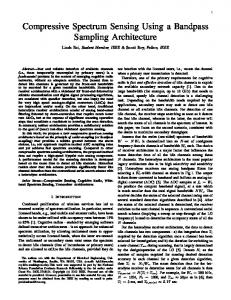
where Tyαm (f ) is determined from (34) using received samples at antenna m. Similar to the BMRC-MSDF detector, the LC-MSDF detector should be robust to both correlated and uncorrelated noise. VI. N UMERICAL R ESULTS In this section, simulation results are presented to provide the insight into the performance of all proposed detectors. We consider flat fading channels for all antennas. Assume that the PU transmits BPSK signals with symbol duration equal to 25 μsec at the carrier frequency of 80 kHz. Unless otherwise stated, we employ the following parameters for all numerical results. The number of antenna at the SU is 2. The sampling rate used is 320 kHz. The number of observed samples is 4000. To estimate the cyclic SDF, we set P = 4 and Ns = 100. The false alarm probability is set to 0.1. Figure 1 shows the performance of the blind channel estimation in spatially correlated noise scenario. Let us define the spatial correlation coefficient as ρ = E{nH i nj }, where ni and nj are column vectors containing noise samples at antenna i and j, respectively. In the simulation, we set ρ = 0 and 0.5. For the cyclic AF, τ = 4. Let us call the cyclic AF when τ = 0 and α = 0 as the conventional AF. We use “Perfect”, “Cyclic”, and “Conv” for perfect estimation, and blind estimation using the cyclic AF and conventional AF, respectively. Only the result of the BMRC-MSDF is shown here for clarity. The result verifies that the blind channel estimation using the cyclic AF provides superior performance than that employing the conventional AF when ρ = 0. When ρ = 0, the cyclic AF and conventional AF have comparable performance. The performance of all detectors in white noise scenario are shown in Figure 2. As expected, pre-combining detectors provide superior results to post-combining detectors since they exploit the channel information. The best detector turns

This full text paper was peer reviewed at the direction of IEEE Communications Society subject matter experts for publication in the IEEE DySPAN 2010 proceedings

TABLE I T HE FALSE ALARM PROBABILITY FOR ALL DETECTORS IN CORRELATED NOISE SCENARIO .

1

Perfect (ρ = 0) Cyclic (ρ = 0) Conv (ρ = 0) Perfect (ρ = 0.5) Cyclic (ρ = 0.5) Conv (ρ = 0.5)

0.9 0.8 0.7

P

d

0.6

(a) Pre-combining detectors BMRC-SCF (Algo. 1) BMRC-SCF (Algo. 2) BMRC-MSDF Pf a

0.067

0.021

0.092

(b) Post-combining detectors

0.5 0.4

Pf a

0.3

LC-SCF (Algo. 3)

LC-SCF (Algo. 4)

LC-MSDF

0.093

0.01

0.064

0.2 0.1

1

0 −20

−15

−10

−5

0.9

0

SNR (dB)

Fig. 1.

0.8

The performance of blind channel estimation based.

0.7

1

0.8

P

d

0.7

0.6 d

BMRC−SCF (Algo. 1) BMRC−SCF (Algo. 2) BMRC−MSDF LC−SCF (Algo. 3) LC−SCF (Algo. 4) LC−MSDF

P

0.9

BMRC−SCF (Algo. 1) BMRC−SCF (Algo. 2) BMRC−MSDF LC−SCF (Algo. 3) LC−SCF (Algo. 4) LC−MSDF

0.5 0.4 0.3

0.6

0.2

0.5

0.1

0.4

0 −20

−15

−10

−5

0

SNR (dB)

0.3

Fig. 3.

0.2

The detection probability for correlated noise scenario.

0.1 0 −20

−15

−10

−5

0

SNR (dB)

Fig. 2.

The detection probability for uncorrelated noise scenario.

out to be the BMRC-MSDF. Even with less computational complexity, it slightly outperforms the BMRC-SCF detector. Among post-combining detectors, it is shown that the LCMSDF provides the best result. This indicates that the proposed modified cyclic SDF can perform well in both detector classes. In Figure 3, the effectiveness of all detectors to temporally correlated noise is investigated. To generate colored noise samples, we pass white noise samples through a temporal correlation filter. The filter used for all antennas is written in a vector form as g1 = [1, 1, 1]. The false alarm probability of pre-combining and post-combining detectors is shown in Table I. All false alarm rates are lower than the pre-determined one, suggesting that all detectors are effective against the effect of noise correlation. It also verifies Lemma 4.2 and Lemma 5.1. For BMRC-SCF detectors, it is observed that Algorithm 1 provides better performance than Algorithm 2 at all SNR

ranges. This is due to the smoothing effect as mentioned in Section IV. As for the LC-SCF, Algorithm 1 performs worse than Algorithm 2 at very low SNR, but starts to achieve better result as SNR increases. It is observed that the performances of detectors employing the modified cyclic SDF are relatively close to those using the cyclic SCF in this case. The effect of the number of antennas on the detection rate is studied in Figure 3 for white noise scenario. For clarity, only the BMRC-MSDF and LC-MSDF detectors are considered in the simulation. The number of antenna, M , is set to 2, 4, and 6. The result shows that as the number of antenna increases, the performance gap between the BMRC-MSDF and LC-MSDF increases. This is because pre-combining detectors achieve higher gain from exploiting more channel knowledge, while post-combining detectors have no channel information to take advantage of. VII. C ONCLUSIONS In this paper, cyclostationarity-based detectors are considered for spectrum sensing in multi-antenna cognitive radio systems. The cyclic SCF and modified cyclic SDF are used as cyclostationary features in signal detection. Pre-combining detectors based on the BMRC, called the BMRC-SCF and

This full text paper was peer reviewed at the direction of IEEE Communications Society subject matter experts for publication in the IEEE DySPAN 2010 proceedings

where (b) is from the following.   |bm am |2   |bm am |2  |bm am |2 = − 2 2 2   m m m

1 0.9

m =m

m

0.8

=

−

2 m m   |am bm |2 = . 2  m

0.7

P

d

0.6

 |bm am |2 m

2

m =m

0.5

R EFERENCES

BMRC−MSDF (M = 6) LC−MSDF (M = 6) BMRC−MSDF (M = 4) LC−MSDF (M = 4) BMRC−MSDF (M = 2) LC−MSDF (M = 2)

0.4 0.3 0.2 0.1 −20

−15

−10

−5

0

SNR (dB)

Fig. 4.

  |bm am |2

The effect of the number of antenna on the detection probability.

BMRC-MSDF detectors, are proposed. To estimate channel coefficients, the eigenvalue-based blind channel estimation exploiting the cyclic AF is considered. For post-combining detectors, linear combiner is incorporated with the considered features to provide the LC-SCF and LC-MSDF detectors. Analysis is given to prove the built-in ability of the cyclic SCF to handle the noise uncertainty and noise correlation. All detectors are shown to be effective in both uncorrelated and correlated noise scenarios. Pre-combining detectors perform better than post-combining ones since the channel knowledge is exploited. It is observed that detectors using the modified cyclic SDF can achieve comparable performance with less computational complexity compared to those using the cyclic SDF.

VIII. A PPENDIX



Defining am = Gm f + α2 and bm = Gm f − magnitude squared of G can be expressed as

α 2



, the

  |am |2 |bm |2 + m m =m am b∗m a∗m bm    2 2 2 2 m |am | |bm | + m m =m |am | |bm |

 |G|2 ≤

m

(a)

≤ 1,

where (a) is from the fact that

  |am bm |2 + |bm am |2

 

∗ ∗

 a b a b  m m m m ≤

2 m m =m

m m =m

(b)

=

  m

m =m

|am |2 |bm |2 ,

[1] J. Mitola, “Cognitive radio: an integrated agent architecture for software defined radio”, PhD Dissertation, KTH, Stockholm, Sweden, Dec. 2000. [2] S. Haykin, “Cognitive radio: brain-empowered wireless communications,” IEEE J. Sel. Areas Commun., vol. 23, no. 2, pp. 201-220, Feb. 2005. [3] Federal Communications Commission, “Notice of proposed rule making and order: Facilitating opportunities for flexible, efficient, and reliable spectrum use employing cognitive radio technologies,” FCC 03-322, Dec. 2003. [4] T. Yucek, and H. Arslan, “A survey of spectrum sensing algorithms for cognitive radio applications,” IEEE Commun. Surveys & Tutorials, vol. 11, no. 1, pp. 116-130, First Quarter, 2009. [5] Y. Zeng, Y.-C. Liang, A. T. Hoang, and R. Zhang “A review on spectrum sensing for cognitive radio: challenges and solutions,” EURASIP Journal on Advances in Signal Processing, to appear. [6] R. Tandra, and A. Sahai, “Fundamental limits on detection in low SNR under noise uncertainty,” WirelessComm, pp. 464-469, June 2005. [7] R. Tandra, and A. Sahai, “SNR walls for signal detection,” IEEE Journal of Selected Topics in Signal Processing, vol. 2, pp. 4-17, Feb. 2008. [8] Y. Zeng, and Y.-C. Liang, “Eigenvalue-based spectrum sensing algorithms for cognitive radio ,” IEEE Trans. Commun., vol. 57, no. 5, pp. 17841793, May 2009. [9] Y. Zeng, Y.-C. Liang, and R. Zhang, “Blindly combined energy detection for spectrum sensing in cognitive radio,” IEEE Signal Process. Letters, vol. 15, pp. 649-652, 2008. [10] W. A. Gardner, Statistical Spectral Analysis: A Nonprobabilistic Theory, Englewood Cliffs, NJ: Prentice-Hall, 1987. [11] E. Teletar, “Capacity of multi-antenna Gaussian channels,” European Transactions on Telecommunications, vol. 10, no. 6, pp. 585-595, Nov./Dec. 1999. [12] G. J. Foschini, and M. J. Gans, ”On the limits of wireless communication in fading environment when using multiple antennas,” Wireless Personal Communication, vol. 6, pp. 311-335, Mar. 1998. [13] X. Chen, W. Xu, Z. He, and X. Tao, “Spectral correlation-based multiantenna spectrum sensing technique,” Proc. IEEE Wireless Commun. and Networking Conf. (WCNC), pp. 735-740, April 2008. [14] R. Mahapatra, and M. Krusheel, “Cyclostationary detection for cognitive radio with multiple receivers,” Proc. IEEE International Symp. Wireless Commun. Systems (ISWCS), pp. 493-497, Oct. 2008. [15] W. A. Gardner, “Measurement of spectral correlation,” IEEE Trans. Acoustics, Speech, and Signal Processing, vol. ASSP-34, no. 5, pp. 11111123, Oct. 1986. [16] A. Papoulis, Probability, Random Variables and Stochastic Processes , McGraw-Hill, 1991. [17] K. Kim, I. A. Akbar, K. K. Bae, J.-S. Um, C. M. Spooner, and J. H. Reed, “Cyclostationary approaches to signal detection and classification in cognitive radio,” Proc. IEEE International Symp. New Frontiers Dynamic Spectrum Access Networks (DySPAN), pp. 212-215, April 2007. [18] A. Fehske, J. Gaeddert, and J. H. Reed, “A new approach to signal classification using spectral correlation and neural networks,” Proc. IEEE International Symp. New Frontiers Dynamic Spectrum Access Networks (DySPAN), pp. 144-150, Nov. 2005. [19] H. Liu, D. Yu, and X. Kong, “A New Approach to Improve Signal Classification in Low SNR Environment in Spectrum Sensing,” IEEE Conf. Cognitive Radio Oriented Wireless Networks and Commun. (CrownCom), pp. 1-5, May 2008.