choices available during the coding and pooling stages: hard assignment vs. ...
typically local image descriptors (SIFT, for example) and they vary in number ....
We present in Section 3 perhaps the simplest approach for adding spatial ...
inferior to LLC [7], NBNN [9], and sparse coding SPM [2]. ..... PAMI 32 (2010)
1271–83.
Spatially Local Coding for Object Recognition Sancho McCann and David G. Lowe Department of Computer Science, University of British Columbia
Abstract. The spatial pyramid and its variants have been among the most popular and successful models for object recognition. In these models, local visual features are coded across elements of a visual vocabulary, and then these codes are pooled into histograms at several spatial granularities. We introduce spatially local coding, an alternative way to include spatial information in the image model. Instead of only coding visual appearance and leaving the spatial coherence to be represented by the pooling stage, we include location as part of the coding step. This is a more flexible spatial representation as compared to the fixed grids used in the spatial pyramid models and we can use a simple, whole-image region during the pooling stage. We demonstrate that combining features with multiple levels of spatial locality performs better than using just a single level. Our model performs better than all previous single-feature methods when tested on the Caltech 101 and 256 object recognition datasets.
1
Introduction
Models based on histograms of visual word frequencies have been quite successful for object recognition, delivering good results on varied datasets. The spatial pyramid was introduced by Lazebnik et al. [1] to allow the representation to account for the spatial distribution of these visual features. In this model, visual features are coded across elements of a visual vocabulary, and these codes are pooled into histograms at several spatial granularities. Many improvements have been made to the original spatial pyramid model. These include replacing nearest neighbor vector quantization with sparse coding [2] or localized soft assignment [3] and replacing average pooling with maxpooling in each spatial bin [4, 5, 3, 2]. Boureau et al. [4] analyzed the various choices available during the coding and pooling stages: hard assignment vs. soft assignment, average pooling vs. max-pooling, and the linear kernel vs. the histogram intersection kernel. It is useful to view these approaches in the context of how each method attends to spatial locality and appearance locality. Prior to spatial pyramids, the bag-of-features method [6] enforced appearance locality in the coding step by its nearest-neighbor vector quantization. Using only a whole-image pooling region, it did not enforce any spatial locality. The spatial pyramid introduced spatial locality using a spatially hierarchical pooling stage. The sparse coding spatial pyramid method [2] takes a different approach to appearance locality that
2
Sancho McCann and David G. Lowe
can select very different bases for patches that are visually similar [7]. Boureau et al. [5] re-instated stricter appearance locality by modifying the pooling stage to enforce to appearance locality. Table 1 presents a taxonomy of these methods based on how they attend to appearance and spatial locality.
Table 1: A taxonomy of histogram-based recognition models focusing on how they attend to appearance and spatial locality. Spatially local coding moves spatial locality into the coding step. Method Bags-of-features [6] Spatial pyramid [1] Sparse coding [2] LLC [7] “Ask-the-locals” sparse coding [5] Spatially local coding (this work)
Appearance locality Coding Coding Sparse coding Local coding Sparse coding + Pooling Coding
Spatial locality Pooling Pooling Pooling Pooling Coding
In contrast to the spatial pyramid approaches, we explore moving the task of enforcing spatial locality into the coding step. We first present more detail about the related spatial pyramid methods. Then we present our method, tuning and implementation details, and finally, experimental results on Caltech 101 and Caltech 256.
2 2.1
Related Methods The Coding/Pooling Pipeline
As our method relates closely to the previous bag-of-features and spatial pyramid approaches, we will explain our method in the context of these other methods. This will facilitate comparisons with these approaches in Section 6. We adopt the coding/pooling framework of Boureau et al. in which all the bag-of-features and spatial pyramid methods can be seen as various choices for a coding and pooling step. Given an image I, we first do feature extraction: Φ(I) : I 7→ {(φ1 , x1 , y1 ), (φ2 , x2 , y2 ), . . . (φnI , xnI , ynI )}. The features φi are typically local image descriptors (SIFT, for example) and they vary in number from image to image (nI ). The pixel location at which feature i is centered is (xi , yi ). After we extract features, we code them using some coding function g((φi , xi , yi )). In previous work, this coding function has included nearest neighbor vector quantization, sparse coding, soft assignment, and localized soft assignment. In bagsof-features and spatial pyramid methods, the coding has been limited to the appearance portion of the descriptor φi , such that g((φi , xi , yi )) = (ˆ g (φi ), xi , yi ). That is, the extracted descriptor’s appearance is converted into a coded version, still associated with the original pixel location.
Spatially Local Coding for Object Recognition
3
We’ll now give some concrete examples of the appearance coding function gˆ for the coding methods just mentioned. In these examples, assume that we have constructed a dictionary D of k appearance elements. This is often referred to as a codebook, and the elements called codewords. For nearest neighbor vector quantization, we use a 1-of-k coding: � gˆ(φi ) = [ui1 , ui2 , . . . , uik ] :
uij =
1 if j = argmina kφi − Da k, 0 otherwise
(1)
For soft assignment, demonstrated by van Gemert et al. [8], a feature is coded across many codebook elements instead of just one:
gˆ(φi ) = [ui1 , ui2 , . . . , uik ] :
exp(−βkφi − Dj k2 ) uij = Pk 2 a=1 exp(−βkφi − Da k )
(2)
where β is a parameter controlling how widely the assignment distributes the weight across all the codewords. A small β gives a broad distribution, while a large β gives a peaked distribution, more closely approximating hard assignment. This is further improved by Liu et al. [3], who use localized soft assignment. Instead of distributing the weight across all codebook elements, they confine the soft assignment to a local neighborhood around the descriptor being coded. Let NN(κ) (φi ) be the set of κ nearest neighbors to φi in D. Then, the localized soft assignment coding is:
gˆ(φi ) = ui = [ui1 , ui2 , . . . , uik ] :
uij = Pk
exp(−βd(φi , Dj )
a=1
� d(φi , Dj ) =
kφi − Dj k2 ∞
exp(−βd(φi , Da ))
(3)
if Dj ∈ NN(κ) (φi ) otherwise
Sparse coding ([2], [4]) codes a descriptor by using the coefficients of a linear combination of the codewords in D, with a sparsity-promoting l1 norm: gˆ(φi ) = ui = argmin kφi − Duk22 + λkuk1
(4)
u∈Rk
Locality constrained linear coding (LLC) is similar, but adds a penalty for using elements of the codebook that have a large Euclidean distance from the descriptor being coded [7]. After choosing one of the above coding functions for gˆ, we obtain the coding for every descriptor extracted from an image: g((φi , xi , yi )) = (ui , xi , yi ). The pooling stage combines these coded features within an image region into a histogram. This histogram hm associated with spatial pooling region Sm is obtained using a pooling function: hm = f ({ui |(xi , yi ) ∈ Sm }).
(5)
4
Sancho McCann and David G. Lowe
The structure of the spatial pooling regions S varies between methods. In the bag-of-features approach of Csurka et al. [6], there is just a single spatial pooling region—one comprising the entire image. In the spatial pyramid, there are several spatial pooling regions—one comprising the entire image and additional regions that split the image into quadrants and even finer subdivisions. Previous work has chosen between two options for the pooling function: average-pooling and max-pooling. Average-pooling produces a histogram that represents the average value of u within a spatial pooling region. Max-pooling instead takes the maximum value of each dimension of u within a spatial pooling region. P {i|(xi ,yi )∈Sm } ui (6) havg m = |{(xi , yi ) ∈ Sm }| hmaxm = [hm1 , hm2 , . . . , hmk ]
where
hmj = max{uij |(xi , yi ) ∈ Sm }
(7)
The final image representation used by the classifier is a concatenation of those histograms hm : H = [h1 h2 . . . hM ] 2.2
(8)
Other Spatial Models
We present in Section 3 perhaps the simplest approach for adding spatial information to the local features, but first, we outline relevant previous work that has attempted to account for the spatial layout of visual features. Boiman et al., in their Naive Bayes nearest neighbor work [9], append a weighted location to the feature vectors, which matches our approach. However, in contrast with the coding/pooling pipeline, they do not quantize features using a codebook. They instead maintain an index of all features extracted from the training data. Zhou et al. [10] use a mixture of Gaussians to model visual appearance, followed by spatially hierarchical pooling of the local features’ membership in each of the mixture’s components. This is essentially a variant of the spatial pyramid model where soft codeword assignment is performed via a Gaussian mixture model, and better results have been achieved by spatial pyramids using localized soft assignment coding and max-pooling [3]. Krapac et al. [11] introduced a compact Fisher vector coding to encode spatial layout of features. They first learn an appearance codebook using k-means or a mixture of Gaussians. Then, for each appearance component, they learn a mixture of Gaussians to represent its spatial distribution. While their representation is more compact, their evaluation shows marginal (if any) improvement over SPM in terms of classification accuracy. Oliveira et al. introduced a method called sparse spatial coding [12]. In their work, they code a descriptor using sparse codebook elements nearby in descriptor
Spatially Local Coding for Object Recognition
5
space. In this sense, it is very close to LLC [7]. In contrast to our work, despite their method’s name, sparse spatial coding is local in descriptor space, not pixel space. As a separate contribution, they introduce a new learning stage called Orthogonal Class Learning that results in better performance than the standard SVM classifier. However, that work is complementary to the work improving the coding/pooling pipeline. Their results using the standard SVM classifier are inferior to LLC [7], NBNN [9], and sparse coding SPM [2].
3
Spatially Local Coding
Our method differs from the previous coding/pooling methods in that we choose a coding function g that directly handles spatial locality, and use a single, wholeimage pooling region during the pooling stage. Instead of choosing g(φi , xi , yi ) = (ˆ g (φi ), xi , yi ), we simultaneously code φi and the location (xi , yi ). In the standard models, φi = [φi1 , φi2 , . . . , φid ]. In spatially local coding, we introduce use a (λ) location-augmented descriptor: φi = [φi1 , φi2 , . . . , φid , λxi , λyi ]. Where λ ∈ R is a location weighting factor giving the importance of the location in feature matching. For example, hard assignment, nearest neighbor vector quantization becomes: � (λ) (λ) 1 if j = argmina k[φi − Da k, g(φi , xi , yi ) = ui : uij = (9) 0 otherwise where we have constructed the codebook D(λ) by k-means clustering over a set of location-augmented descriptors and locations extracted from the training data. All of the coding functions presented in Section 2 can use the locationaugmented descriptors in place of the standard appearance-only descriptors. In summary, spatially local coding uses location-augmented feature vectors, and a single, whole-image spatial pooling region, because the features themselves already carry sufficient spatial information. We have moved the task of maintaining spatial locality into the coding stage. Previously, this has been left for the pooling stage. One advantage of spatially local coding is that we avoid having to commit to artificial grid boundaries to define the spatial pooling regions. Other authors have had to work around this by experimenting with alternate binning geometries to engineer one that performs well for their problem [13], or supervised learning of optimal pooling regions from an over-complete set of rectangular bins [14]. Both of these methods keep the responsibility for spatial locality in the pooling stage. Instead, our λ parameter defines a receptive field associated with each codebook element. 3.1
Multi-level Spatially Local Coding
The λ parameter plays an important role in our model. If we set λ = 0, we revert to the standard bag-of-features representation. If we set λ to be high, we learn
6
Sancho McCann and David G. Lowe
Average class accuracy
features that are very strictly localized. Figure 1 shows that it is possible to determine a somewhat optimal setting for λ (approximately 1.5 for the Caltech 101 dataset). However, the specific λ may depend on the particulars of the dataset. Instead of committing to a single λ, we build several codebooks, each with a different λ, and code image features across all of the codebooks simultaneously. This is similar in spirit to having multiple levels in the spatial pyramid, with each level dividing space into finer and finer regions. Table 2 shows that this combination is beneficial. 0.70 0.65 0.60 0.55 0.50 0.45 0.40 0.35 0.30 0.25 2 10
Caltech 101 (15 training images) 1.50 3.00 0.75 0.00
λ = 0.00 λ = 0.75 λ = 1.50 λ = 3.00
104 103 Codebook dimensions
105
Fig. 1: The performance of single-codebook SLC is dependent on the choice of λ. Regardless of the choice of λ, the optimal codebook dimensionality is similar. Based on this observation, we can choose to use the same dimensionality across all of the codebooks in a multi-λ model.
Table 2: The experimental setting of these results is explained in detail in Section 6. This shows that the combination of multiple codebooks, each with a different λ-weighting, produces higher classification accuracy than any of the codebooks individually. Codebook (8192D) λ = 0.00 λ = 0.75 λ = 1.50 λ = 3.00 4-level (linear kernel)
Caltech 101 (15 training) 52.4 ± 0.4 61.1 ± 0.2 66.5 ± 0.5 64.9 ± 0.3 68.4 ± 0.2
Figure 2 shows the types of features learned by our system. For this visualization, we choose a particular category and determine the per-codeword weights derived from the linear SVM model (the SVM training is described further in Section 6). These are the codewords that most signal the presence of the object
Spatially Local Coding for Object Recognition
7
of interest. We show the distribution of features found in the training images that match the top-weighted codewords. The SVM can choose between unlocalized and highly localized features.
killer-whale
sunflower
dice
car-side
zebra
Fig. 2: Visualization of top-ranked features (hand-picked from among the top ten) for five of the object categories. The top row is the spatial distribution of each codeword and the second row is the average appearance of each codeword (as in Fig. 3). The subsequent rows show where occurrences of the codewords are centered in particular training images. Looking down each column shows that these codewords tend to be associated with particular parts or textures.
4
Optimal Codebook Size and Model Size
In [1], Lazebnik et al. reported their model reached optimal performance for Caltech 101 with approximately 200-400 codewords. We verify that in Fig. 4. We also confirm that localized soft assignment coding [3] achieves superior performance and can effectively make use of more codebook elements. Our model performs even better, but requires more codebook elements (for this figure, we used 4-codebook SLC with λ = 0, 0.75, 1.5, 3.0, localized soft assignment, and max-pooling). These results may seem counter to those reported by Chatfield et al. in [15], who report performance of spatial pyramid methods never decreasing on Caltech 101 as codebook size grew up to 8,000 dimensions. However, those results were shown for a much denser SIFT sampling density than used in our experimental setups. We extract single-scale SIFT every 8 pixels. Chatfield et al. extracted SIFT at 4 scales every 2 pixels, resulting in approximately 64× the descriptors
Sancho McCann and David G. Lowe
car-side
dice
saturn
8
Fig. 3: Each pair of rows is a visualization of the top ten features from an object category. The scatter-plots show the spatial distribution of each codeword, while the grey-scale snippets show their average appearance.
as in our experimental setting. In Section 6, we show some results at higher extraction densities and note that at higher densities, the optimal codebook dimensionality is higher. We hypothesize that Chatfield et al. had not reached that optimal dimensionality for their extremely dense extraction setting. Our results match those by Boureau et al. [4] who reported that on Caltech 101, optimal codebook size is relatively low for hard assignment coding, higher for soft assignment coding, and higher when extraction densities increase. These trends are also observed by van Gemert et al. [8]. Comparing the required codebook size is useful, as it points to a potential increase in the computational cost of the coding phase, but comparing the resulting model size is also useful, as this affects the computational cost of learning and testing. In 3-level spatial pyramid models, the model dimensionality is 21× the size of the codebook. This is due to the 21 spatial pooling regions (1 whole-image region, 2 × 2 regions in the second level, and 4 × 4 regions at the third level). Figure 4 also compares the methods based on their model dimensionality, not just their codebook size. 4-codebook SLC produces better classification accuracy than a state-of-the-art spatial pyramid at comparable model dimensionalities.
5
Efficient Codebook Construction
As highlighted in the previous section, the codebook size used by our model is significantly larger than those used by spatial pyramid methods. Efficient codebook construction becomes important. The standard algorithm for k-means takes O(nkd) per iteration, where n is the number of data points (SIFT features) being clustered into k clusters and d is the data dimensionality. We used two approximations in our implementation of k-means to achieve efficient clustering.
Average class accuracy
Spatially Local Coding for Object Recognition
0.70 0.68 0.66 0.64 0.62 0.60 0.58 0.56 0.54 2 10
9
Caltech 101 (15 training images): Codebook and model dimensionality vs. accuracy
Original SPM (3-levels, intersection kernel) Localized soft assignment (3-levels, intersection kernel) SLC (4-codebooks, linear kernel)
104 103 Codebook dimensionality
105
103
104 Model dimensionality
10
0.70 0.68 0.66 0.64 0.62 0.60 0.58 0.56 50.54
Fig. 4: We compare the performance of the original spatial pyramid model with the localized soft assignment variant and our SLC model. The localized soft assignment performs better than the original and requires larger codebook sizes for optimal performance. Our SLC model achieves even better performance, but requires even more codebook dimensions. When comparing the model dimensionalities (21× the size of the codebook to account for the spatial pyramid bins, or 4× the size of the codebook to account for our 4-codebook SLC), SLC outperforms the others at the equivalent model dimensionalities.
First, we use FLANN (Fast Library for Approximate Nearest Neighbors) [16] to perform approximate assignment of data points to clusters during each iteration of k-means. FLANN automatically selects and tunes its approximate nearest neighbor search algorithm to the particulars of the dataset in order to achieve a specified accuracy with maximum efficiency. This is similar to the approximate k-means described by Philbin et al. in [17], but with more precise control of the approximation error. Figure 5 shows how classification performance and construction time is affected by changing FLANN’s approximation accuracy. Second, we have observed a small improvement in classification accuracy by using the kmeans++ [18] initialization method rather than random initialization. However, this initialization method is expensive, so we use a subsampled kmeans++ initialization that does not significantly affect our results. Instead of performing kmeans++ initialization using all descriptors being clustered, we do kmeans++ initialization using a random 10% of the descriptors. This gives the benefit of an improved initialization at a fraction of the cost. When using subsampled kmeans++ initialization instead of full kmeans++ initialization, construction time (clustering 1,000,000 descriptors into a 4096-dimensional codebook) with 95% accuracy drops from 37 minutes to 20 minutes. At 80% accuracy, the construction time drops from 23 minutes to 12 minutes. Note that exact kmeans using full kmeans++ initialization requires approximately 240 minutes in this
10
Sancho McCann and David G. Lowe 0.510
23 min
Classification accuracy
0.505 0.500
18 min
0.495
16 min
0.490 0.485
37 min 240 min
15 min
0.480 0.4750.0
0.2
0.4 0.6 K-means approximation accuracy
0.8
1.0
Fig. 5: Codebooks produced by approximate k-means give similar classification accuracies as codebooks produced by the exact k-means algorithm. The construction time for several data points is shown. In this experiment, we clustered 1,000,000 features into 4096 codewords to use in a bag-of-features model. Initialization was with kmeans++. The dataset was Caltech 101, using 15 training images per category. (Dataset details are in Section 6.)
setting (see Fig. 5). We use 90% target accuracy and subsampled kmeans++ in all of our following experiments.
6
Experiments
We compare spatially local coding against a variety of state-of-the-art spatial pyramid variants on Caltech 101 [19] and Caltech 256 [20].1 We resize Caltech 101 and Caltech 256 images to fit inside a 300 × 300 pixel square. This is consistent with the published results we compare against. We compared methods using 15 and 30 training images per category for Caltech 101, and using 30 training images per category for Caltech 256, all common points of reference from the literature. We first learn a codebook using a random subsampling of 1,000,000 descriptors from the training set. This is an appearance-only codebook for all of the spatial pyramid methods. For our SLC method, we learn multiple spatially local codebooks, with λ = {0, 0.75, 1.50, 3.00}. Then, we form the spatial pyramid or SLC representations of the training images. For our implementation of the original spatial pyramid, we use nearestneighbor vector quantization and average pooling in three spatial pyramid levels, as in [1]. For our implementation of the localized soft assignment spatial pyramid, we use soft assignment over the ten nearest codebook elements, and max-pooling in three spatial pyramid levels as in [3]. For our SLC model, we also use soft assignment over the ten nearest codebook elements from each λ-level, and maxpooling over a global spatial pooling region. In [3], they showed results motivating 1
Code is available at http://www.cs.ubc.ca/projects/spatially-local-coding for ease of comparison.
Spatially Local Coding for Object Recognition
11
Classification accuracy
a small neighborhood, with ten neighbors being the optimal for Caltech 101. We confirmed that this still holds in our codebooks. We learn for each class a one-vs-all SVM (using the LibSVM library), selecting the regularization parameter via cross-validation. For each run of the experiment, we record the average class accuracy over 101 or 256 classes (ignoring the background class as suggested by [20]). We experimented with both the linear SVM and histogram intersection kernels SVM, but found that the linear SVM outperforms the histogram intersection kernel for our model (see Fig. 6). Thus, in Table 3, the results shown for our SLC model are obtained using a linear SVM.
45.5 45.0 44.5 44.0 43.5 43.0 42.5 42.0 41.5
Caltech 256 (30 training images)
72.0 Caltech 101 (15 training images) 71.5 71.0 70.5 70.0 Linear Intersection 69.5 69.0 8192 16384 32768 65536 8192 16384 32768 65536 SLC codebook dimensionality SLC codebook dimensionality
Fig. 6: Our model yields best results with a linear SVM. Only at low dimensionalities on Caltech 256, where the performance of both SVM types is low, does the intersection kernel outperform the linear SVM. At optimal codebook dimensionalities, our model’s performance using a linear SVM dominates the performance of the histogram intersection kernel.
All of our reported numbers are based on 10 repetitions of the experiment, each time selecting a different training/testing split, building new codebooks, and learning new models. We report the mean and standard error of the mean. The methods we compare against have generally published their results based on single-scale 16x16 SIFT features [21] using the VLFeat implementation [22] extracted every 8 pixels [1, 3, 4, 2]. We perform the majority of our comparisons at this setting as well. We re-implement the original spatial pyramid method [1] and the best performing state-of-the-art variant, localized soft assignment [3] so as to provide a head-to-head comparison based on our extracted features. To report the classification accuracy achieved by our re-implementations, we ran them at various dimensionalities, since their performance is dependent on codebook dimensionality, and we report the highest result we could achieve with the other methods. Despite our results on SLC being obtained at higher codebook dimensionalities, this comparison is fair, since the model dimensionalities are comparable (see Fig. 4), and performance only deteriorates for the other methods as we increase their codebook size. Table 3 shows that spatially local coding achieves better classification accuracy than all previous alternatives using single-scale SIFT features on Caltech 101 and Caltech 256.
12
Sancho McCann and David G. Lowe
Boureau et al. [5] have reported higher accuracy than any of the other previous methods. However, they achieve these results using a denser SIFT sampling (every 4 pixels), and use a feature based on the concatenation of 4 individual SIFT features within a small region which they call macrofeatures. We set these results aside from the rest of the reported numbers to highlight this difference, and run a separate comparison where we also extract SIFT every 4 pixels (however, we don’t construct their macrofeatures). Spatially local coding again achieves a higher classification accuracy. Wang et al. [7] use another slightly different feature set for their experiments on locality constrained linear coding. They extract multiscale features (HOG) every 8 pixels at three different sizes. We again set these reported results aside from the rest and run a separate comparison. While the above comparisons are sufficient to demonstrate SLC’s superior performance as compared to state-of-the-art spatial pyramids, we provide an additional evaluation at an even denser extraction setting, extracting multiscale SIFT every 4 pixels. These experiments show that spatially local coding outperforms all previous spatial pyramid methods for object recognition on Caltech 101 and Caltech 256. We have shown this in the setting of single-scale and multi-scale SIFT features, at two different extraction densities. In addition, we have provided a detailed survey and comparison of the previously published results, making clear how they are comparable with each other or not. To the best of our knowledge, any previous work reporting higher accuracy than ours combines together multiple complimentary feature types.
6.1
Notes on Timing
Codebook construction scales logarithmically with the number of codebook dimensions, because we use approximate matching at each k-means step. SLC’s multiple codebook construction can be multi-threaded, giving elapsed real time for codebook construction that scales logarithmically with the number of codebook dimensions. Vector quantization also scales logarithmically with the number of codebook dimensions and linearly with the number of codebooks. To code 7680 training images (for Caltech 256), 1024D SPM required 2 minutes. SLC using four 16384D codebooks takes 11 minutes. That is 5.5x the compute time, despite the model size being 64x as large. SVM training is the bottleneck regardless of the approach. This time is unaffected by switching from local soft assignment SPM to SLC. Both use soft assignment across a small number of nearest neighbors, giving sparse feature vectors. Gram matrix construction for Caltech 256’s 7680 training images took 55 minutes using local soft assignment SPM with 8192D, and 50 minutes under SLC using four 8192D dictionaries. Doubling the SLC dimensionality to 16384D increased the gram matrix construction time to 65 minutes.
Spatially Local Coding for Object Recognition
13
Table 3: Results on Caltech 101 (using 15 and 30 training examples per class) and 256 (using 30 training examples per class). We compare our SLC method against previously published figures and against re-implementations of the original spatial pyramid and localized soft assignment tested on our feature set. The numbers we report for our re-implementations of previous methods are the best results we could achieve from among a range of codebook dimensionalities. Bold method names show our experiments; the others are from the literature. Cal. 101 (15)
Original SPM [1] Original SPM (ours) Localized soft assignment [3] Localized soft assignment (ours) Sparse Coding SPM [2] Sparse Coding SPM [4] SLC [8192d × 4] SLC [16384d × 4]
56.4 57.8 ± 0.3 66.2 ± 0.4 67.0 ± 0.45 68.4 ± 0.2 68.3 ± 0.3
LLC [7] (HOG) Localized soft assignment [3] (SIFT) SLC [8192d × 4] SLC [16384d × 4] SLC [32768d × 4] SLC [65536d × 4]
65.43 71.4 ± 0.4 72.5 ± 0.3 70.9 ± 0.4 69.6 ± 0.3
Boureau et al. [5] SLC [8192d × 4] SLC [16384d × 4] SLC [32768d × 4] SLC [65536d × 4]
71.0 ± 0.3 71.1 ± 0.3 71.6 ± 0.4 -
SLC [65536d × 4]
72.7 ± 0.4
7
Cal. 101 (30) Single-scale SIFT features extracted every 8 pixels 64.6 ± 0.8 65.2 ± 0.4 74.21 ± 0.81 72.2 ± 0.3 73.2 ± 0.54 71.8 ± 1.0 75.5 ± 0.4 75.7 ± 0.4 Multi-scale features extracted every 8 pixels 73.44 76.48 ± 0.71 78.0 ± 0.4 79.2 ± 0.2 77.2 ± 0.6 77.5 ± 0.4 Single-scale SIFT features extracted every 4 pixels 77.3 ± 0.6 77.6 ± 0.2 78.9 ± 0.2 79.6 ± 0.8 Multi-scale SIFT features extracted every 4 pixels 81.0 ± 0.2
Cal. 256 (30)
30.0 ± 0.4 37.2 ± 0.2 34.02 ± 0.35 38.9 ± 0.3 40.0 ± 0.2
41.19 41.8 ± 0.3 43.4 ± 0.2 44.3 ± 0.1 43.4 ± 0.3
41.7 ± 0.8 41.9 ± 0.2 43.5 ± 0.3 44.6 ± 0.2 45.1 ± 0.2
46.6 ± 0.2
Conclusion
Spatially local coding is a simpler and more flexible way to enforce spatial locality in histogram-based object models than previous approaches. By simultaneously coding appearance and location, we remove the necessity of a complicated pooling stage to adequately model the spatial locations of visual features. We have shown that a combination of location-augmented codebooks gives better classification accuracy than spatial pyramid models. The large codebook dimensionality required by our models potentially poses extra computational cost, but we have shown approximations that speed up the codebook construction process and an evaluation of the effect of those approximations on classification accuracy. We have presented these results alongside a useful survey of previously published results and our re-implementations of previous results. To the best of our knowledge, we have shown the highest classification accuracy achieved on Caltech 101 and Caltech 256 using a single visual feature type.
14
Sancho McCann and David G. Lowe
References 1. Lazebnik, S., Schmid, C., Ponce, J.: Beyond Bags of Features: Spatial Pyramid Matching for Recognizing Natural Scene Categories. CVPR (2006) 2. Yang, J., Yu, K., Gon, Y., Huang, T.: Linear spatial pyramid matching using sparse coding for image classification. In: CVPR. (2009) 3. Liu, L., Wang, L., Liu, X.: In Defense of Soft-assignment Coding. In: ICCV. (2011) 4. Boureau, Y.L., Bach, F., LeCun, Y., Ponce, J.: Learning mid-level features for recognition. In: CVPR. (2010) 5. Boureau, Y.L., Le Roux, N., Bach, F., Ponce, J., LeCun, Y.: Ask the locals: multi-way local pooling for image recognition. In: ICCV. (2011) 6. Csurka, G., Dance, C., Fan, L., Willamowski, J., Bray, C.: Visual categorization with bags of keypoints. In: Workshop on Statistical Learning in Computer Vision, ECCV. (2004) 7. Wang, J., Yang, J., Yu, K., Lv, F., Huang, T., Gong, Y.: Locality-constrained linear coding for image classification. In: CVPR. (2010) 8. van Gemert, J.C., Veenman, C.J., Smeulders, A.W.M., Geusebroek, J.M.: Visual word ambiguity. PAMI 32 (2010) 1271–83 9. Boiman, O., Shechtman, E., Irani, M.: In defense of nearest-neighbor based image classification. In: CVPR. (2008) 10. Zhou, X., Cui, N., Li, Z., Liang, F., Huang, T.S.: Hierarchical Gaussianization for Image Classification. (2009) 11. Krapac, J., Verbeek, J., Jurie, F.: Modeling spatial layout with Fisher vectors for image categorization. In: ICCV. (2011) 12. Oliveira, G.L., Nascimento, E.R., Vieira, A.W., Campos, M.F.: Sparse Spatial Coding: A Novel Approach for Efficient and Accurate Object Recognition. In: ICRA. (2012) 13. Laptev, I., Marszalek, M., Schmid, C.: Learning realistic human actions from movies. In: CVPR. (2008) 14. Jia, Y., Huang, C.: Beyond Spatial Pyramids : Receptive Field Learning for Pooled Image Features. In: NIPS 2011 Workshop on Deep Learning and Unsupervised Feature Learning. (2011) 15. Chatfield, K., Lempitsky, V., Vedaldi, A.: The devil is in the details: an evaluation of recent feature encoding methods. In: BMVC. (2011) 16. Muja, M., Lowe, D.: Fast approximate nearest neighbors with automatic algorithm configuration. In: VISSAPP. (2009) 17. Philbin, J., Chum, O., Isard, M., Sivic, J., Zisserman, A.: Object retrieval with large vocabularies and fast spatial matching. In: CVPR. (2007) 18. Arthur, D., Vassilvitskii, S.: k-means ++ : The Advantages of Careful Seeding. In: Eighteenth Annual ACM-SIAM Symposium on Discrete Algorithms (SODA), New Orleans, Louisiana, Society for Industrial and Applied Mathematics (2007) 1027–1035 19. Fei-Fei, L., Fergus, R., Perona, P.: Learning generative visual models from few training examples: An incremental Bayesian approach tested on 101 object categories. In: Workshop on Generative-Model Based Vision, CVPR. (2004) 20. Griffin, G., Holub, A., Perona, P.: Caltech-256 Object Category Dataset. Technical report, California Institute of Technology (2007) 21. Lowe, D.G.: Distinctive Image Features from Scale-Invariant Keypoints. IJCV 60 (2004) 91–110 22. Vedaldi, A., Fulkerson, B.: VLFeat: An open and portable library of computer vision algorithms (www.vlfeat.org) (2008)