move), one should note that there is a class of applications where ... number of related auxiliary data types, such as pure spatial or temporal types, ..... branches, offices, plants, or stores of a company; coal mines, oil wells, being used for some ... estate (changes of shape only through legal acts), agricultural land use, etc.
Spatio-Temporal Data Types: An Approach to Modeling and Querying Moving Objects in Databases*
Martin Erwig 1 Ralf Hartmut Güting 1 Markus Schneider 1 Michalis Vazirgiannis 1+2
1) Praktische Informatik IV Fernuniversität Hagen D-58084 Hagen GERMANY
2) Computer Science Division Dept. of Electr. and Comp. Engineering National Tech. University of Athens Zographou, Athens, 15773 GREECE
Abstract: Spatio-temporal databases deal with geometries changing over time. In general, geometries cannot only change in discrete steps, but continuously, and we are talking about moving objects. If only the position in space of an object is relevant, then moving point is a basic abstraction; if also the extent is of interest, then the moving region abstraction captures moving as well as growing or shrinking regions. We propose a new line of research where moving points and moving regions are viewed as three-dimensional (2D space + time) or higher-dimensional entities whose structure and behaviour is captured by modeling them as abstract data types. Such types can be integrated as base (attribute) data types into relational, object-oriented, or other DBMS data models; they can be implemented as data blades, cartridges, etc. for extensible DBMSs. We expect these spatio-temporal data types to play a similarly fundamental role for spatio-temporal databases as spatial data types have played for spatial databases. The paper explains the approach and discusses several fundamental issues and questions related to it that need to be clarified before delving into specific designs of spatiotemporal algebras.
December 1997
*
This research was supported partially be the CHOROCHRONOS project, funded by the EU under the Training and Mobility of Researchers Programme, contract no. ERB FMRX-CT96-0056.
–
1
1
–
Introduction
In the past, research in spatial and temporal data models and database systems has mostly been done independently. Spatial database research has focused on supporting the modeling and querying of geometries associated with objects in a database [Gü94]. Temporal databases have focused on extending the knowledge kept in a database about the current state of the real world to include the past, in the two senses of “the past of the real world” (valid time) and “the past states of the database” (transaction time) [TCG+93]. Nevertheless, many people have felt that the two areas are closely related, since both deal with “dimensions” or “spaces” of some kind, and that an integration field of “spatio-temporal databases” should be studied1 and would have important applications. The question is, what the term spatio-temporal database really means. Clearly, when we try an integration of space and time, we are dealing with geometries changing over time. In spatial databases, three fundamental abstractions of spatial objects have been identified: A point describes an object whose location, but not extent, is relevant, e.g. a city on a large scale map. A line (meaning a curve in space, usually represented as a polyline) describes facilities for moving through space or connections in space (roads, rivers, power lines, etc.). A region is the abstraction for an object whose extent is relevant (e.g. a forest or a lake). These terms refer to two-dimensional space, but the same abstractions are valid in three or higher-dimensional spaces. Now, considering points, the usual word for positions or locations changing over time is move. Regions may change their location (i.e. move) as well as their shape (grow or shrink). Hence we conclude that spatio-temporal databases are essentially databases about moving objects. Since lines (curves) are themselves abstractions or projections of movements, it appears that they are not the primary entities whose movements should be considered, and we should focus first on moving points and moving regions. In the approach described in this paper we will consider the fundamental properties of moving points and moving (and evolving) regions and try to support their treatment in data modeling and querying, rather than be driven by particular (existing) applications. On the other hand, if we succeed in providing such basic support, then we may be able to initiate applications that so far have never been thought of. Table 1 shows a list of entities that can move, and questions one might ask about their movements. Although we focus on the general case of geometries that may change in a continuous manner (i.e. move), one should note that there is a class of applications where geometries change only in discrete steps. Examples are boundaries of states, or cadastral applications, where e.g. changes of ownership of a piece of land can only happen through specific legal actions. Our proposed way of modeling is general and includes these cases, but for them also more traditional strategies could be used, and we shall compare the approaches in the paper. Also, if we consider transaction time (or bitemporal) databases, it is clear that changes to geometries happen only in discrete steps through updates to the database. Hence it is clear that the description of moving objects refers first of all to valid time. So we assume that complete descriptions of moving objects are put into the database by the applications, which means we are in the framework of histo1
This is in fact the goal of the EU-TMR-Project CHOROCHRONOS under which this work was done.
–
2
–
rical databases reflecting the current knowledge about the past of the real world. Transaction time databases about moving objects may be feasible, but will not be considered initially. Moving Points
Moving Regions
People: •Movements of a terrorist/spy/criminal Animals •Determine trajectories of birds, whales, … •Which distance do they traverse, at which speed? How often do they stop? •Where are the whales now? •Did their habitats move in the last 20 years? Stars •All the astronomical stuff Cars •Taxis: Which one is closest to a passenger request position? •Trucks: Which routes are used regularly? •Did the trucks with dangerous goods come close to a high risk facility? Planes •Were any two planes close to a collision? •Are two planes heading towards each other (going to crash)? •Did planes cross the air territory of state X? •At what speed does this plane move? What is its top speed? •Did Iraqi planes cross the 39th degree? Ships •Are any ships heading towards shallow areas? •Find “strange” movements of ships indicating illegal dumping of waste. Rockets, missiles, tanks, submarines •All kinds of military analyses
Countries •What was the largest extent ever of the Roman empire? •On which occasions did any two states merge? (Reunification, etc). •Which states split into two or more parts? •How did the Serb-occupied areas in former Yugoslavia develop over time? When was the maximal extent reached? Was Ghorazde ever part of their territory? Forests, Lakes •How fast is the Amazone rain forest shrinking? •Is the dead sea shrinking? What is the minimal and maximal extent of river X during the year? Glaciers •Does the polar ice cap grow? Does it move? •Where must glacier X have been at time Y (backward projection)? Storms •Where is the tornado heading? When will it reach Florida? High/low pressure areas •Where do they go? Where will they be tomorrow? Scalar functions over space, e.g. temperature •Where has the 0-degree boundary been last midnight? People •Movements of the celts etc. Troops, armies •Hannibal going over the alps. Show his trajectory. When did he pass village X? Cancer •Can we find in a series of X-ray images a growing cancer? How fast does it grow? How big was it on June 1, 1995. Why was it not discovered then? Continents •History of continental shift.
Table 1: Moving objects and related queries There is also an interesting class of applications that can be characterized as artifacts involving space and time, such as interactive multimedia documents, virtual reality scenarios, animations, etc. The techniques developed here might be useful to keep such documents in databases and ask queries related to the space and time occurring in these documents. The purpose of this paper is to describe and discuss an approach to modeling moving and evolving spatial objects based on the use of abstract data types. Essentially, we introduce data types for moving points and moving regions together with a set of operations on such entities. One needs also a number of related auxiliary data types, such as pure spatial or temporal types, time-dependent real numbers, and so forth. This collection of types and operations can then be integrated into any DBMS object algebra or query language to obtain a complete data model and query language. The goal of this first paper on the approach is not yet to offer a specific design of such types and operations or a formal definition of their semantics. This needs to be done in further steps. Instead, here the goal is to give an outline of the work that should be done, to justify the approach in the light of possible alternatives, and to discuss a number of basic design choices that need to be made before delving into the specific designs.
–
3
–
There has been a large body of work on spatial and on temporal databases. We discuss the basic approaches taken in these fields within Section 3. Not so many papers have addressed the integration of space and time. We discuss this more specific research in Section 5. The paper is structured as follows: Section 2 explains the basic idea of spatio-temporal data types in a bit more detail. Section 3 is devoted to discussing basic questions regarding the approach as well as some fundamental design choices that need to be made. Section 4 briefly describes the steps to be taken following the approach proposed here. Section 5 discusses related work, and Section 6 offers conclusions.
2
The Basic Idea
Let us assume that a database consists of a set of object classes (of different types or schemas). Each object class has an associated set of objects; each object has a number of attributes with values drawn from certain domains or atomic data types. Of course, there may be additional features, such as object (or oid-) valued attributes, methods, object class hierarchies, etc. But the essential features are the ones mentioned above; these are common to all data models and already given in the relational model. We now consider extensions to the basic model to capture time and space. As far as objects are concerned, an object may be created at some time and destroyed at some later time. So we can associate a validity interval with it. As a simplification, and to be able to work with standard data models, we can even omit this validity interval, and just rely on time-dependent attribute values described next. Besides objects, attributes describing geometries changing over time are of particular interest. Hence we would like to define collections of abstract data types, or in fact many-sorted algebras containing several related types and their operations, for spatial values changing over time. Two basic types are mpoint and mregion. Let us assume that purely spatial data types called point and region are given that describe a point and a region in the 2D-plane2 (a region may consist of several disjoint areas which may have holes) as well as a type time that describes the valid time dimension. Then we can view the types mpoint and mregion as mappings from time into space, that is mpoint: time → point mregion: time → region More generally, we can introduce a type constructor τ which transforms any given atomic data type α into a type τ(α) with semantics τ(α) : time → α and we can denote the types mpoint and mregion also as τ(point) and τ(region), respectively. A value of type mpoint describing a position as a function of time can be represented as a curve in the three-dimensional space (x, y, t) shown in Figure 1. We assume that space as well as time dimen-
2
We restrict attention to movements in 2D space, but the approach can, of course, be used as well to describe timedependent 3D space.
–
4
–
sions are continuous, i.e., isomorphic to the real numbers. (It should be possible to insert a point in time between any two given times and ask for e.g. a position at that time.) t
y
x Figure 1: A moving point A value of type mregion is a set of volumes in the 3D space (x, y, t). Any intersection of that set of volumes with a plane t = t0 yields a region value, describing the moving region at time t0. Of course, it is possible that this intersection is empty, and an empty region is also a proper region value. The algebra with the types mpoint and mregion may have operations such as mpoint × mpoint
→ mreal
mdistance
which computes the distance between the two moving points at all times and hence returns a time changing real number, a type that we call mreal (“moving real”). Another operation could be mpoint × mregion
→ mpoint
visits
which returns the positions of the moving point given as a first argument at the times when it was inside the (possibly) moving region provided as a second argument. Here it becomes clear that a value of type mpoint may also be a partial function, in the extreme case a function where the point is undefined at all times. Operations may also involve pure spatial or pure temporal types and other auxiliary types. For the following examples, let line be a data type describing a curve in 2D space which may consist of several disjoint pieces; it may also be self-intersecting. Let us also have operations mpoint line mreal mreal
→ line → real → real → time
trajectory length minvalue, maxvalue mintime, maxtime
Here trajectory is the projection of a moving point onto the plane, and length returns the total length of a line value. Minvalue and maxvalue give the minimum and maximum values of a moving real. Mintime and maxtime return the times when the value was minimal or maximal (for the moment we ignore the problem that these may not be uniquely defined).
–
5
–
These data types can now be embedded into any DBMS data model as attribute data types, and the operations be used in queries. For example, we can integrate them into the relational model and have a relation planes (airline: string, id: string, flight: mpoint) We can then ask a query “Give me all flights of Lufthansa longer than 5000 kms”: SELECT airline, id FROM planes WHERE airline = "Lufthansa" AND length (trajectory (flight)) > 5000 Whereas this query just uses projection into space, there are also genuine spatio-temporal questions that can not be solved on projections. For example, “Find all pairs of planes that during their flight came closer to each other than 500 meters!”: SELECT p.airline, p.id, q.airline, q.id FROM planes p, planes q WHERE minvalue (mdistance (p.flight, q.flight)) < 0.5 This is in fact an instance of a spatio-temporal join.
3
Some Fundamental Issues and Choices
Given this proposal of an approach to spatio-temporal modeling and querying, several basic questions arise that need to be clarified before proceeding in this direction: • How is this related to the approaches taken in spatial databases and in temporal databases? • Is it not sufficient to simply plug in spatial data types into temporal databases? • We have seen spatio-temporal data types that are mappings from time into spatial data types. Is this realistic? How can we store them? Don’t we need finite, discrete representations? • If we use discrete representations, what do they mean? Are they observations of the moving objects? • If we use discrete representations, how do we get the infinite entities from them that we really want to model? What kind of interpolation should be used? In the following subsections we discuss these questions. 3.1
The Spatial vs. the Temporal Database Approach
The proposed approach is in fact quite similar to what has been done in spatial databases so far. There, a database is viewed as a collection of object classes; objects may or may not have attributes of spatial data types. Research has then tried to identify “good” designs of collections of types and operations, or algebras (e.g. [SV89, SH91, GS95]). As far as the DBMS is concerned, spatial data types are in principle not different from other data types. Of course, they need special support in indexing, join methods, etc., but this might also happen to other data types. So the proposal of spatio-temporal data types directly continues the spatial DB approach.
–
6
–
The obvious question is whether one could not equally well, or perhaps better, extend the approach taken in temporal databases. The following is surely a simplification, but should in essence be true: in temporal databases the emphasis has been on considering databases as containing collections of facts rather than objects. Hence a tuple in a relation is basically a fact. A normal database contains facts that describe what is now believed in the database to be the current state of the real world. To obtain temporal databases, tuples are extended with time stamps that associate either a valid time interval (historical databases) or a transaction time interval (rollback databases), or both (bitemporal databases) [SA85, Sn87]. A valid time interval expresses when this fact was true in the real world; a transaction time interval shows when the fact was believed in the database. Hence we get, for example, relations like the following: employee (name: string, salary: int || from, to, begin, end) It is important to note that time stamps are system-defined and maintained attributes rather than userdefined as in spatial databases. In a temporal database of some flavor (e.g. historical), every relation has these (e.g. valid time) attributes. This makes sense, since time is a universal concept that applies to all facts in a database. Because time is so general that it affects all facts of the database, it definitely makes sense to let the system deal with it as far as possible automatically. Hence the user does not have to specify time attributes when creating a new relation schema, and in querying, a lot of effort has been invested to make sure that these system-maintained attributes behave naturally. For example, performing a join on two tables, the system automatically puts only tuples together that are valid at the same time. Also, if the user is not interested in the time aspects and does not mention them in a query, the behaviour should be consistent with that of a standard database (these issues are known as upward compatibility, snapshot reducibility, support of legacy applications, etc. [BJ96]). Because a user does not declare and see explicit time attributes, there is no big incentive to offer e.g. time intervals with a number of operations in the style of abstract data types that would then be used like other data types in querying (although some work in this direction exists [Lo93]). Rather, special query language extensions are provided to allow the user to refer to and describe relationships between the implicit time attributes. If we try to extend this approach in a straightforward way to integrate space, we could add a systemmaintained spatial attribute (e.g. a region) to each tuple. But what would that mean? To be consistent with the fact-based interpretation, it should mean that this is the region in space where this fact is true. There may be a few applications with facts whose truth varies over space. But the vast majority of facts is independent of space. Hence on the whole, it does not seem the right approach to associate a system-defined spatial attribute with each tuple. We have discussed only the perhaps most popular approach of using tuple time stamps. There is also work in temporal databases proposing attribute time stamps, that is, describe the development of an attribute value by giving a set of (time-interval, value) pairs, or a sequence of (time, value) pairs [CC87, GV85, Ga88]. In fact, at an abstract level these approaches view attribute values as functions from time into some domain, as we do here. Hence this is not so far from our proposal of spatiotemporal data types. Also the time sequences approach [SS87] appears much more closely related than tuple time stamps.
– 3.2
7
–
Why Not Just Use “Temporal Databases With Spatial Data Types”
Here the idea is quite simple: take any temporal data model or DBMS with its system-maintained time attribute(s), and enhance it by offering spatial data types with operations to be used as user-defined attributes, as in spatial databases. For example, we may have a valid-time relation: country (name: string, area: region || from, to) Each tuple describes the extent of a country during a certain period of time. Whenever a country’s boundaries change, this is recorded in another tuple. This is something like the cross product of temporal and spatial databases. Capabilities of spatial and temporal systems are combined without any specific integration effort. This approach is natural and reasonable, and it appears that its technology is already well-understood, as techniques from the two fields can be used. However, it is limited to certain classes of spatio-temporal applications and also has some other drawbacks, as we will see. As far as data modeling is concerned, this kind of model can essentially describe stepwise constant values. To understand its scope, let us first introduce a classification of spatio-temporal applications. 3.2.1
Classes of Applications
We characterize applications with respect to their “shape” in the three-dimensional space (2D space, time). For example, (point, point) means a point in space and a point in time. (1) Events in space and time – (point, point). Examples are archeological discoveries, plane crashes, volcano eruptions, earth quakes (at a large scale where the duration is not relevant). (2) Locations valid for a certain period of time – (point, interval). Examples are: cities built at some time, still existing or destroyed; construction sites (e.g. of buildings, highways); branches, offices, plants, or stores of a company; coal mines, oil wells, being used for some time; or “immovables”, anything that is built at some place and later destroyed. (3) Set of location events – sequence of (point, point). Entities of class (1) when viewed collectively. For example, the volcano eruptions of the last year. (4) Stepwise constant locations – sequence of (point, interval). Examples are: the capital of a country; the headquarter of a company; the accomodations of a traveler during a trip; the trip of an email message (assuming transfer times between nodes are zero). (5) Moving entities – moving point. Examples are people, planes, cars, etc., see Table 1. (6) Region events in space and time – (region, point). E.g, a forest fire at large scale. (7) Regions valid for some period of time – (region, interval). For example, the area closed for a certain time after a traffic accident. (8) Set of region events – sequence of (region, point). For example, the Olympic games viewed collectively, at a large scale. (9) Stepwise constant regions – sequence of (region, interval). For example, countries, real estate (changes of shape only through legal acts), agricultural land use, etc. (10) Moving entities with extent – moving region. For example, forests (growth); forest fires at small scale (i.e. we describe the development); people in history; see Table 1.
– 3.2.2
8
–
Suitability of this Approach
As far as describing the structure of data is concerned, the approach of using “temporal databases with spatial data types” (SDT-TDB for short) can naturally describe application classes (1) through (4) and (6) through (9). But it cannot capture any kind of movement, that is, classes (5) and (10). On the other hand, our proposal of spatio-temporal data types is entirely general and can easily describe all ten classes of applications. If we consider operations on data, then SDT-TDBs have difficulty to support queries that refer to the development of an entity over time, for example, “What was the largest extent of a country ever?” or “Find travelers that move frequently!”. Such questions have to be translated into operations on sets of tuples, and the first step is always to retrieve all tuples describing the entity. Apart from being inefficient, defining operations on sets of tuples and integrating these into a query language as well as into query processing is difficult. Viewing the time-dependent geometry as an entity and an ADT as we propose seems much cleaner and simpler. There is also a problem if the object with the stepwise constant spatial attribute changes frequently with respect to other attribute values. In that case, a fresh version of the tuple needs to be created whenever the other attribute value changes. Traditional temporal database research has assumed that attribute values have small representations. This is not true for spatial entities, which may have quite large descriptions. Hence if we keep many copies of the spatial attribute, just because another attribute changes, then a lot of storage is wasted. One can try to avoid this by vertical decomposition of such relations, but this, of course, has also its drawbacks, as joins are needed to put tuples together again. In summary, this approach is valid and can support some applications, but also has its problems. Spatio-temporal data types support in addition all kinds of movements, and avoid the mentioned problems. So they seem preferable even for those applications that can be treated with SDT-TDBs. 3.3
Continuous vs. Discrete Modeling
What does it mean to develop a data model with spatio-temporal data types? Actually, this is a design of a many-sorted algebra. There are two steps: 1.
Invent a number of types and operations between them that appear to be suitable for querying. So far these are just names, which means one gives a signature. Formally, the signature consists of sorts (names for the types) and operators (names for the operations).
2.
Define semantics for this signature, that is, associate an algebra, by defining carrier sets for the sorts and functions for the operators. So the carrier set for a type t contains the possible values for t, and the functions are mappings between the carrier sets.
For a formal definition of many-sorted signature and algebra see [EM85] or [Gü93]. Now it is important to understand that one can make such designs at two different levels of abstraction, namely as continuous or as discrete models.
– 3.3.1
9
–
Continuous Models Are Beautiful …
Continuous models allow us to make definitions in terms of infinite sets, without worrying whether finite representations of these sets exist. This allows us to view a moving point as a continuous curve in the 3D space, as a mapping from an infinite time domain into an also infinite space domain. All the types that we get by application of the type constructor τ are functions over an infinite domain, hence each value is an infinite set. Please note carefully that by continuous model we do not mean any model to describe a continuous curve. Continuous curves or shapes can certainly be described by discrete models. The crucial point is that the continuous model does not care whether finite representations exist and just talks about the infinite point sets. This continuous view is the conceptual model that we are interested in. The curve described by a plane flying over space is continuous; for any point in time there exists a value. A region may have a smooth boundary, and a moving region be a smooth shape in 3D. In Section 2 we have in fact described the types mentioned under this view. In a continuous model, we have no problem in using types like “moving real”, mreal, and operations like mpoint × mpoint
→ mreal
mdistance
since it is quite clear that at any time some distance between the moving points exists (when both are defined). It is also easy to introduce an operation velocity: → mpoint
mpoint
velocity v This is just the derivative of the time-dependent vector r (t )giving the position of the moving point, ∂ v v r (t ), usually denoted as r˙ (t ) , which is a time-dependent vector again and hence matches that is, ∂t the type mpoint. Defining formally an algebra for a continuous model looks as follows. As mentioned above, we need to define carrier sets for the types (sorts) and functions for the operators. For a type t, we denote its carrier set as A t and for an operator op the function giving its semantics as fop. We consider the following example signature: sorts point, time, real, mpoint, mreal operators mpoint × time → point mpoint × mpoint → mreal
attime mdistance
Here attime is the operation that gives us the position of the moving point at the specified time. We first define the carrier sets: Apoint
:= IR2 ∪ {⊥}
A time
:= IR ∪ {⊥}
A real
:= IR ∪ {⊥}
Ampoint := {f | f: Atime → Apoint is a function} Amreal := {f | f: Atime → Areal is a function}
–
10
–
So a point is an element of the plane over real numbers, or undefined. 3 For the “moving” types one could also provide a single generic definition based on the type constructor τ introduced in Section 2: ∀α ∈ {point, real, …}:
Aτ(α) := {f | f: Atime → Aα is a function}
Functions are defined as follows. Let r, s be values of type mpoint and t a time. fattime (r, t)
:=
r(t)
fmdistance (r, s) := g: Atime → Areal such that
d (r (t ), s(t )) if r (t ) ≠ ⊥ ∧ s(t ) ≠ ⊥ g(t) = otherwise ⊥
where d(p, q) denotes the Euclidean distance between two points in the plane. So continuous models are conceptually simple and their semantics can be defined relatively easily. 3.3.2
… But Only Discrete Models Can Be Implemented
The only trouble with continuous models is that we cannot store and manipulate them in computers. Only finite and in fact reasonably small sets can be stored; data structures and algorithms have to work with discrete representations. From this point of view, continuous models are entirely unrealistic; only discrete models are usable. A discrete model can of course describe an infinite set (i.e. have an infinite set as its semantics). For example, an interval is given by two real numbers [a, b], but the meaning is the infinite set of real numbers in between. A discrete model can also use polynomials or other functions to describe a smooth curve or surface. This means we somehow need discrete models for moving points and moving regions as well as for all other involved types (mreal, region, …). We can view discrete models as approximations, finite descriptions of the infinite shapes we are interested in. In spatial databases there is the same problem of giving discrete representations for in principle continuous shapes; there almost always linear approximations have been used. Hence, a region is described in terms of polygons and a curve in space (e.g. a river) by a polyline. Linear approximations are attractive because they are easy to handle mathematically; most algorithms in computational geometry work on linear shapes such as rectangles, polyhedra, etc. A linear approximation for a moving point is a polyline in 3D space; a linear approximation for a moving region is a set of polyhedra (see Figure 2). Remember that a moving point can be a partial function, hence it may disappear at times, the same is true for the moving region. Defining formally an algebra for a discrete model means the same as for the continuous model: Define carrier sets for the sorts and functions for the operators. We consider a part of the example above: sorts point, time, real, mpoint operators mpoint × time → point 3
attime
We include the value ⊥ (undefined) into all domains to make the functions associated with operators complete. This is more practical than have the system return an error when evaluating a partial function.
–
11
t
– t
y
y
x
x
Figure 2: Discrete representations for moving points and moving regions Type mreal and operator mdistance have been omitted; for good reason, as we will see. Carrier sets can be defined as follows: Apoint
:= Dpoint ∪ {⊥}
where Dpoint = real × real
A time
:= Dtime ∪ {⊥}
where Dtime = real
A real
:= real ∪ {⊥}
Ampoint := { | m ≥ 0, ( ∀1 ≤ i ≤ m : pi ∈ Dpoint , ti ∈ Dtime , bi ∈ bool, ci ∈ bool), ( ∀i, j ∈ {1, …, m}: i < j ⇒ ti < t j ) } A few explanations are needed. Here by “real” and “bool” we mean data types offered by a programming language. We have introduced names for the defined part of a carrier set, e.g. Dpoint. A moving point is represented by a sequence of quadruples. The sequence may be empty; this will mean that the position is undefined at all times. Each quadruple contains a position in space pi and a time ti. It also contains a flag bi which tells whether the point is defined at times between ti and ti+1 (bi = true). This allows for the representation of partial functions (of the conceptual level). Finally, there is a flag ci which states whether between ti and ti+1 a stepwise constant interpretation is to be assumed, i.e., the point stayed in pi, did not move (ci = true), or linear interpolation, i.e., a straight line between pi and pi+1, is to be used (ci = false). This representation has been chosen in order to support all classes of applications for moving points (1) through (5) of Section 3.2.1, e.g. unique events, stepwise constant locations, etc. Note that this particular model does not allow one to represent linear interpolation over a (half) open interval, e.g. use linear interpolation on [ti, ti+1) with points pi and pi+1 and then have a different value p' to be valid at time ti+1. Linear models are more deeply discussed in [ESG97]. The intended meaning of the structure that we have just described needs of course to be formalized. This is exactly the semantics of the operator attime: Let r be a value of type mpoint and t a time value. Let r = for some m ≥ 0.
–
12
–
fattime (r, t) := ⊥ ⊥ pi lin( pi , ti , pi +1 , ti +1 , t ) p i ⊥
if m = 0 if m > 0 ∧ (t < t1 ∨ t > tm ) if m ≥ 1 ∧ (∃i ∈{1, ..., m} : ti = t ) if m ≥ 2 ∧ (∃i ∈{1, ..., m − 1} : (ti < t < ti +1 ) ∧ bi = true ∧ ci = false ) if m ≥ 2 ∧ (∃i ∈{1, ..., m − 1} : (ti < t < ti +1 ) ∧ bi = true ∧ ci = true ) if m ≥ 2 ∧ (∃i ∈{1, ..., m − 1} : (ti < t < ti +1 ) ∧ bi = false )
where lin( p1 , t1 , p2 , t2 , t ) is a function that performs linear interpolation (puts a line through the two points (p1, t1) and (p2, t2) in 3D space and returns the point p on the line at time t). One can observe that definitions for the discrete model are considerably more complex than those for the continuous model. On the other hand, they can be translated into data structures and algorithms which is not the case for the continuous model. Apart from complexity, there are other difficulties with discrete modeling. Suppose we wish to define the type mreal and the operation mdistance. What is a discrete representation of the type mreal ? Since we like linear approximations for the reasons mentioned above, the obvious answer would be to use a sequence of pairs (value, time) and use linear interpolation between the given values, similarly as for the moving point. Then an mreal value would look as shown in Figure 3. (For one-dimensional values depending on time it is more natural to use a horizontal time axis.) v
t Figure 3: Discrete model of a moving real If we now try to define the mdistance operator mpoint × mpoint
→ mreal
mdistance
we have to determine the time-dependent distance between two moving points represented as polylines. To see what that means, imagine that through each vertex of each of the two polylines we put a plane t = ti parallel to the xy-plane. In three dimensions this is hard to draw; so we show it just in the x and t dimensions in Figure 4a. Within each plane t = ti we can easily compute the distance; this will result in one of the vertices for the resulting mreal value. Between two adjacent planes we have to consider the distance between two line segments in 3D space (see Figure 4b). However, this is not a linear but a quadratic function (moving along the time axis, the distance may decrease and then increase again).
–
13
–
t
t
y
x (a)
x (b)
Figure 4: (a) Laying planes through vertices of a moving point; (b) two segments passing in 3D This is annoying, especially since the minimal distance between two moving points can be much smaller than the distance measured in any of the planes t = ti. Hence using just these measurements as vertices for the moving real and then use linear interpolation would lead to quite wrong results. What can be done? One can either stick with linear interpolation and then add as vertices the focal points of the parabolas describing the time-dependent distance between two planes. In this way at least the minimal distance would not be missed. However, then the discrete model would already be inconsistent in itself, as the behaviour of the distance between the two polylines is not correctly represented. An alternative would be to define the discrete model for the moving real in such a way, that it contains parameters for quadratic functions between two vertices. But this immediately raises other questions. Why just quadratic functions motivated by the mdistance operation, perhaps other operations need other functions? Should we allow parameters for polynomials? Up to what degree? Storing these parameters is expensive. And all kinds of operations that we need on moving reals must then be able to deal with these functions. We have discussed this example in some detail to make clear what kind of nasty problems arise in discrete modeling that we simply do not see in continuous modeling. This is certainly not the only example, we will discuss a similar problem below. Nevertheless, ultimately only discrete models are implementable. 3.3.3
Both Levels of Modeling Are Needed
As a conclusion of the discussion in this section, it seems clear that both levels of modeling are indispensable. For the discrete model this is clear anyway, as only discrete models can be implemented. However, if we restrict attention directly to discrete models, there is a danger that a conceptually simple, elegant design of query operations is missed. This is because the representational problems might lead us to prematurely discard some options for modeling. For example, from the discussion above one might conclude that moving reals are a problem and no such type should be introduced. But then, instead of operations minvalue, maxvalue, mintime, maxtime (see Section 2) on moving reals one has to introduce corresponding operations for each time-dependent numeric property of a moving object. Suppose we are interested in distance between two moving points, speed of a moving point, and size and perimeter of a moving region. Then we need operators mindistance, maxdistance, mindistancetime, maxdistancetime, minspeed,
–
14
–
maxspeed, and so forth (16 operations instead of 4+4 with moving reals). Clearly, this leads to a proliferation of operators and to a bad design of a query language. So we feel a good strategy is to start with a design at the continuous level, and then to aim for that target when designing discrete models. 3.4
Discrete Models: Observations vs. Description of Shape
Looking at the sequence of 3D points describing a moving point in a discrete model, one may believe that these are observations of the moving object at a certain position at a specific time. This may or may not be the case. Our view is that it is, first of all, an adequate description of the shape of a continuous curve (i.e., an approximation of that curve). We assume that the application has complete knowledge about the curve, and puts into the database a discrete description of that curve. What is the difference to observations? Observations could mean that there are far too many points in the representation, for example, because a linear movement over an hour happens to have been observed every second. Observations could also be too few so that arbitrarily complex movements have happened between two recorded points; in that case our (linear or other) interpolation between these points could be arbitrarily wrong. Hence we assume that the application, even if it does make observations, employs some preprocessing of observations and also makes sure that enough observations are taken. Note that it is quite possible that the application adds points other than observations to a curve description, as it may know some physical laws governing the movements of this particular class of objects. The difference in view becomes even more striking if we consider moving regions. We require the application to have complete knowledge about the 3D shape of a moving region so that it can enter into the database the polyhedron (or set of polyhedra) as a good approximation. In contrast, observations could only be a sequence of region values. But whereas for moving points it is always possible to make a straight line interpolation between two adjacent positions, there is no way that a database system could, in general, deduce the shape of a region between two arbitrary successive observations. For example, two observations may look as shown in Figure 5. This region has split and one of the resulting parts has developed a hole. t
y
x Figure 5: Two observations of a moving region Hence, it is the job of the application to make enough observations and otherwise have some knowledge how regions of this kind can behave and then apply some preprocessing in order to produce a reasonable polyhedral description. How to get polyhedra from a sequence of observations, and what
–
15
–
rules must hold to guarantee that the sequence of observations is “good enough” may be a research issue in its own right. We assume this is solved when data are put into the database. 3.5
Discrete Models: Linear vs. Nonlinear Functions for Shape Description
In a discrete model one can describe the shape of a continuous curve (e.g. a moving point) by either linear functions (a polyline) or other functions. In Section 3.3.2 we have explained why linear functions are attractive, and we have used linear interpolation in the example model. However, it is also possible to use, for example, higher order polynomials, and this has also certain advantages. Technically, the model of Section 3.3.2 describes a moving point by a sequence of 3D points, and uses linear interpolation between two adjacent points. But this is entirely equivalent to a model which decomposes the time axis into a sequence of time intervals, and describes the curve within each time interval by giving (the parameters of) a linear function. That is, one interval could be described as ([t', t"], a, b, c, d), meaning that the curve within the interval [t', t"] is r(t) = (x(t), y(t)) with x(t) = at + b, y(t) = ct + d. Similarly, one could use in the model (and later store in a data structure) parameters of other functions. Whereas in any case we are using a piece-wise approximation of the curve to be described, an advantage of higher-order polynomials could be that less pieces are needed, and that perhaps the approximation of the curve within each piece (time interval) could be more precise. Also, linear approximations are a bit unnatural for describing movements. Firstly, movements in most cases do not have sudden bends. Second, if we compute the derivative of linear functions for operations like speed (returning an mreal) or velocity (returning an mpoint), then we get stepwise constant results. If we take the derivative of such a result again (acceleration), it is either 0 (within time intervals) or infinite (at interval boundaries). All of this is quite unnatural. An interesting option might be to allow piece-wise description by (up to) cubic polynomials. They have enough parameters (four) so that one can select independently two slopes and two positions at interval boundaries (see Figure 6). This allows one to describe bends in such a way that the first derivative (speed, velocity) is continuous. x x (t ′) = x ′, x˙ (t ′) = a,
x" x'
x (t ′′) = x ′′, x˙ (t ′′) = b t'
t"
t
Figure 6: Fitting a curve at the boundaries of a time interval Remember that it is the application’s task to produce a good description of the curve, hence we assume here that the application would determine the time intervals as well as the parameters within each time interval and then put this into the database.
–
16
–
Whereas such a model would offer a more natural description of movement and speed, it is not clear into which difficulties it might lead in terms of definition of functions for other operations and of algorithms. Note that the curve so described is the “semantics” of the moving point, and all operations have to be formulated in terms of the positions on that curve. For example, we have to compute the mdistance between two moving points on the curves, or compute the part of the curve inside a polyhedron for the visits operation of Section 2. As mentioned before, most algorithms in computational geometry deal with linear shapes.
4
Design Steps
Our approach to spatio-temporal database systems can be realized by the following steps: Step 1: Clarify the basic assumptions and options. This is what has been done in this paper. Step 2: Make a good design of a continuous model. This consists of two parts: Step 2.1: Determine the signature. This means identify a collection of types and operations, that are (i) simple and easy to use to formulate queries, (ii) have great flexibility and “expressive power” (if not in a formal then at least in a practical sense). To achieve this goal, there are two complementary strategies. (1) Study a sufficiently large number of applications and try to formulate queries that are relevant to them. This will initially often generate new operations and sometimes types, but hopefully the process will converge after some experience. (2) Try to study systematically the relationships between the involved types. For example, look at the relationships between moving point and (i) a point in time, (ii) a region in time (= temporal element, set of intervals), (iii) a point in space, (iv) a region in space. Do the same for moving regions. – In any case, make operations as general as possible. For example, for all “moving” types of the form τ(α) we can have operations to give the domain and the range of this mapping. Step 2.2: Define the algebra. Define the semantics of the signature formally by giving carrier sets for the types (sorts) and functions for the operators, as shown in Section 3.3.1. Step 3: Design a discrete model. Try to find discrete representations for the types designed in Step 2. Perhaps additional types and other operations are needed. Define the discrete model formally by giving carrier sets and functions on them, as shown in Section 3.3.2. Step 4: Design data structures for the types and algorithms for the operations of the discrete model. Here the challenge is to find representations that support many operations well enough rather than finding the optimal data structure for a single algorithm. An analogous problem has been solved for spatial data types in the implementation of the ROSE algebra [GRS95]. As an example, consider the design of a data structure for a moving region modeled as a set of polyhedra. A set of polyhedra can be represented by the set of its faces. A face is a polygon with holes in 3D. It can be represented as an outer cycle plus a set of inner cycles (the holes). Each cycle is a simple polygon which can be represented as a list of vertices (3D points). The task of the attime operation on moving regions is to determine the region value at a given time t0. Essentially the intersection of the set of faces with a plane t = t0 needs to be computed. In a first step,
–
17
–
all faces intersecting this plane must be retrieved. Only faces fi whose time interval [ti, t'i] contains t0 intersect this plane. Hence it is useful to augment the data structure for a moving region by an interval index over the faces, e.g. a segment tree (see [PS85]) so that these faces can be found efficiently. In a second step, the intersection of the face with the plane is computed, yielding one or more line segments. In a third step, line segments are put together to recover the region structure (set of faces with holes in 2D). The database system into which these data structures are to be embedded must offer some facility for the handling of attribute values with a representation of widely varying size. These data structures should be kept in a tuple/object representation if they are small, and in a separate page sequence, if they are large. Such techniques have already been used in spatial DBMS for spatial data types (see [Gü94]). For example, the DBMS can offer an extensible array abstraction for the implementation of data types. The structure of polyhedral faces mentioned above can then be mapped into a few arrays of appropriate sizes; persistent pointers between them are given by array indices. Clearly, it is beyond the scope of this paper to go into more detail here, but this sketch should give some idea of the work to be done in Step 4. Step 5: Implement the design of Step 4 as an extension package to an extensible DBMS (a data blade, cartridge, etc.).
5
Related Work
For several years researchers both in the spatial and in the temporal community have recognized the need of a simultaneous treatment and integration of data with spatial and temporal features in databases. A comprehensive bibliography on spatio-temporal databases until 1994 is given in [ASS94]. Many of its articles document the interaction of space and time through application examples. But nevertheless, up to now research on models for spatio-temporal databases is still in its infancy. Most of the research on this topic has focused on the extension of specialized spatial or temporal models to incorporate the other dimension. Most modeling approaches adopt the snapshot view, i.e., represent space-time data as a series of snapshots. Gadia et al. [GCT93] propose time- and spacestamping of thematic attributes as a method to capture their time- and space-varying values. The time dimension describes when an attribute value is valid, and the spatial dimension expresses where it is valid. While each value has always a temporal evolution, it is doubtful whether it always has a spatial aspect, as discussed in Section 3.1. Worboys [Wo94] defines spatio-temporal objects as so-called spatio-bitemporal complexes. Their spatial features are given by simplicial complexes; their temporal features are described by bitemporal elements attached to all components of simplicial complexes. In [CT95] and [PD95] event-based approaches for ST databases are proposed. Events indicate changes of the locations and shapes of spatial objects and trigger the creation of new versions in the database. All these approaches are only capable of modeling discrete or stepwise constant but not continuous temporal evolutions of spatial data. Yeh and Cambray [YC93, YC95] emphasize some aspects also mentioned in our paper. Since spatial data over time can be highly variable, they consider a continuous view of these data as indispensable and a snapshot view as inappropriate. So-called behavioral time sequences are introduced. Each
–
18
–
element of such a sequence contains a geometric value, a date, and a behavioral function, the latter describing the evolution up to the next element of the sequence. Examples of such user or predefined functions are punctual functions, step functions, linear functions, and interpolation functions. A 2D object evolving in the course of time is described by a 3D object. Boundary representation is used to represent a solid as a union of faces. While there are some similar ideas, they have no notion of abstract spatio-temporal data types with operations. An interesting proposal that directly addresses moving objects is given in [SWC+97]. Here a moving object, e.g. a car or plane, is described by a so-called dynamic attribute. A dynamic attribute contains a motion vector and can describe the current status of a moving object (e.g. heading in a certain direction at a certain speed). An update to the database can change this motion vector (e.g. when a plane takes a turn). In this model a query will return different results when posed at different times; queries about the expected future are also possible. This model is geared towards vehicle tracking applications; in contrast to our proposal attributes do not contain the whole history of a moving object. Several papers in the GIS literature study storage schemes for stepwise changing region values [Kä94, Pr89, RYG94, BM78]. The general idea is to use a start version and then record the changes. Some work addresses spatio-temporal modeling within multimedia documents. In [VTS97] the assumption is that objects are rectangles that appear for some time related spatially and/or temporally with other objects. The temporal relationships are represented by a set of operators that apart from the relationship maintain its causality. This model does not cover motion and does not address arbitrary or changing object shapes. In [NNS97] a model for moving objects in a multimedia scene is proposed. Objects are represented in terms of their trajectory, as discrete snapshots. A set of objects comprises a scene represented as a graph. Edges between object nodes are labeled by spatio-temporal relationships. This model focuses on considering whole scenes and also the evolvement of relationships between objects. It also does not address changes in the shape of objects. Computational geometry has also shown interest in time-varying spatial objects. For instance, [AR92, FL91, GMR91] deal with Voronoi diagrams of moving points. The task is to maintain the Voronoi diagram when a set of points is moving continuously over time.
6
Conclusions
We have proposed a new approach to the modeling and implementation of spatio-temporal database systems based on spatio-temporal data types. This approach allows an entirely general treatment of time-changing geometries, whether they change in discrete steps, or continuously. Hence in contrast to most other work it also supports the modeling and querying of moving objects. Spatio-temporal data types can be used to extend any DBMS data model, and they offer a clear implementation strategy as extension packages to extensible DBMSs. We feel that the paper opens up a new direction of research. As a first step, it is of crucial importance to clarify the underlying assumptions and to understand the available design options. Besides proposing the approach as such, this is the main contribution of this paper. It offers a foundation from which one can now go into specific designs of spatio-temporal algebras at the continuous and discrete level, using linear or nonlinear approximations.
–
19
–
Acknowledgments We are grateful to our partners in the CHOROCHRONOS project for asking many of the questions that have been answered in this paper. Thanks for many clarifying discussions especially to Mike Böhlen, Christian Jensen, Nikos Lorentzos, and Timos Sellis.
References [AR92]
Albers, G., and T. Roos, Voronoi Diagrams of Moving Points in Higher Dimensional Spaces. 3rd Scandinavian Workshop on Algorithm Theory (SWAT'92), LNCS 621, pp. 399-409, 1992.
[ASS94]
Al-Taha, K., R.T. Snodgrass, and M.D. Soo, Bibliography on Spatio-Temporal Databases. A C M SIGMOD Record, vol. 22, pp. 59-67, 1994.
[BJ96]
Böhlen, M.H., and C. Jensen, Seamless Integration of Time into SQL. Dept. of Computer Science, Aalborg University, Technical Report R-96-49, Dec. 1996. Basoglu, U., and J. Morrison, The Efficient Hierarchical Data Structure for the U.S. Historical Boundary File. Harward Papers on GIS, vol. 4, Addison-Wesley, 1978.
[BM78] [CC87] [CT95] [EM85] [ESG97] [FL91]
Clifford, J., and A. Croker, The Historical Relational Data Model (HRDM) and Algebra Based on Lifespans. Proc. 3rd Intl. Conf. on Data Engineering (Los Angeles, CA, 1987), 528-537. Claramunt, C., and M. Thériault, Managing Time in GIS: An Event-Oriented Approach. Recent Advances in Temporal Databases, Springer-Verlag, pp. 23-42, 1995. Ehrig, H., and B. Mahr, Fundamentals of Algebraic Specification I. Springer, Berlin, 1985. Erwig, M., M. Schneider, and R.H. Güting, Temporal and Spatio-Temporal Data Models and Their Expressive Power. FernUniversität Hagen, Informatik-Report 225, December 1997. Fu, J.-J., and R.C.T. Lee, Voronoi Diagrams of Moving Points in the Plane. Int. Journal of Computational Geometry and Applications, vol. 1, no. 1, pp. 23-32, 1991.
[Ga88]
Gadia, S.K., A Homogeneous Relational Model and Query Languages for Temporal Databases. ACM Transactions on Database Systems 13 (1988), 418-448.
[Gü93]
Güting, R.H., Second-Order Signature: A Tool for Specifying Data Models, Query Processing, and Optimization. Proc. ACM SIGMOD Conf. (Washington, 1993), 277-286. Güting, R.H., An Introduction to Spatial Database Systems. VLDB Journal 4 (1994), 357-399.
[Gü94] [GCT93]
Gadia, S.K., V. Chopra, and U.S. Tim, An SQL-Like Seamless Query of Spatio-Temporal Data. Int. Workshop on an Infrastructure for Temporal Databases, pp. Q-1 - Q-20, 1993.
[GMR91] Guibas, L., J.S.B. Mitchell and T. Roos, Voronoi Diagrams of Moving Points in the Plane. 17th Workshop on Graph-Theoretic Concepts in Computer Science, LNCS 570, pp. 113-125, 1991. [GRS95]
[GS95] [GV85] [Kä94] [Lo93] [NNS97] [PD95]
Güting, R.H., Th. de Ridder, and M. Schneider, Implementation of the ROSE Algebra: Efficient Algorithms for Realm-Based Spatial Data Types. Proc. of the 4th Intl. Symposium on Large Spatial Databases (Portland, August 1995), 216-239. Güting, R.H., and M. Schneider, Realm-Based Spatial Data Types: The ROSE Algebra. VLDB Journal 4 (1995), 100-143. Gadia, S.K., and J.H. Vaishnav, A Query Language for a Homogeneous Temporal Database. Proc. ACM Conf. on Principles of Database Systems, 1985, 51-56. Kämpke, T., Storing and Retrieving Changes in a Sequence of Polygons. Int. Journal of Geographical Information Systems, vol. 8, no. 6, pp. 493-513, 1994. Lorentzos, N., The Interval-Extended Relational Model and Its Application to Valid-Time Databases. In [TCG+93], 67-91. Nabil, M., A. Ngu, and J Shepherd, Modeling Moving Objects in Multimedia Database. Proc. of the 5th Conf. on Database Systems for Advanced Applications, Melbourne, Australia, 1997. Peuquet, D.J., and N. Duan, An Event-Based Spatiotemporal Data Model (ESTDM) for Temporal Analysis of Geographical Data. Int. Journal of Geographical Information Systems, vol. 9, no. 1, pp. 7-24, 1995.
– [PS85] [Pr89]
20
–
Preparata, F.P., and M.I. Shamos, Computational Geometry: An Introduction. Springer-Verlag, New York, 1985. Price, S., Modelling the Temporal Element in Land Information Systems. Int. Journal of Geographical Information Systems, vol. 3, no. 3, pp. 233-243, 1989.
[RYG94]
Raafat, H., Z. Yang and D. Gauthier, Relational Spatial Topologies for Historical Geographical Information. Int. Journal of Geographical Information Systems, vol. 8, no. 2, pp. 163-173, 1994.
[Sn87]
Snodgrass, R., The Temporal Query Language TQuel. ACM Transactions on Database Systems 12 (1987), 247-298.
[SA85]
Snodgrass, R., and I. Ahn, A Taxonomy of Time in Databases. Proc. ACM SIGMOD Conf. (Austin, Texas, May 1985), 236-246. [SH91] Svensson, P., and Z. Huang, Geo-SAL: A Query Language for Spatial Data Analysis. Proc. 2nd Intl. Symp. on Large Spatial Databases (Zürich, Switzerland, 1991), 119-140. [SS87] Segev, A., and A. Shoshani, Logical Modeling of Temporal Data. Proc. ACM SIGMOD Conf., San Francisco, 1987, 454-466. [SV89] Scholl, M., and A. Voisard, Thematic Map Modeling. Proc. 1st Intl. Symp. on Large Spatial Databases, Santa Barbara, 1989, 167-190. [SWC+97] Sistla, A.P., O. Wolfson, S. Chamberlain, and S. Dao, Modeling and Querying Moving Objects. Proc. IEEE Intl. Conf. on Data Engineering (Birmingham, U.K., 1997), 422-432. [TCG+93] Tansel, A.U., J. Clifford, S. Gadia, S. Jajodia, A. Segev, and R. Snodgrass (eds.), Temporal Databases: Theory, Design, and Implementation. Benjamin/Cummings Publishing Company, 1993. [VTS97] Vazirgiannis, M., Y. Theodoridis and T. Sellis, Spatio-Temporal Composition and Indexing for Large Multimedia Applications. To appear in Multimedia Systems, 1997. [Wo94] [YC93] [YC95]
Worboys, M.F., A Unified Model for Spatial and Temporal Information. The Computer Journal, vol. 37, no. 1, pp. 27-34, 1994. Yeh, T.S., and B. de Cambray, Time as a Geometric Dimension for Modeling the Evolution of Entities: A 3D Approach. 2nd Int. Conf. on Integrating GIS and Environmental Modeling, 1993. Yeh, T.S., and B. de Cambray, Modeling Highly Variable Spatio-Temporal Data. 6th AustraliAsian Database Conf., p. 221-230, 1995.