Spatio-Temporal Multi-Dimensional Relational Framework Trees

Spatio-Temporal Multi-Dimensional Relational Framework Trees Matthew Bodenhamer School of Computer Science University of Oklahoma Norman, OK, USA [email protected]

Daniel Fennelly Samuel Bleckley Department of Psychology School of Art Reed College University of Oklahoma Portland, OR, USA Norman, OK, USA [email protected] [email protected]

Abstract—The real world is composed of sets of objects that move and morph in both space and time. Useful concepts can be defined in terms of the complex interactions between the multi-dimensional attributes of subsets of these objects and of the relationships that exist between them. In this paper, we present Spatiotemporal Multi-dimensional Relational Framework (SMRF) Trees, a new data mining technique that extends the successful Spatiotemporal Relational Probability Tree models. From a set of labeled, multi-object examples of a target concept, our algorithm infers both the set of objects that participate in the concept and the key object and relation attributes that describe the concept. In contrast to other relational model approaches, SMRF trees do not rely on pre-defined relations between objects. Instead, our algorithm infers the relations from the continuous attributes. In addition, our approach explicitly acknowledges the multi-dimensional nature of attributes such as position, orientation and color. Our method performs well in exploratory experiments, demonstrating its viability as a relational learning approach. Keywords-relational learning; continuous multi-dimensional attributes; multiple instance learning; spatial representations

I. M OTIVATION AND BACKGROUND The world is composed of collections of objects, each with a set of associated attributes. Whether it is a robot preparing to perform the next step in a cooking sequence or an agent generating warnings of severe weather, only a specific subset of the observable objects is relevant to making decisions about what steps to take next. In particular, the relevance of an object is determined by its attributes and the relations that it has with other objects. These attributes are often continuous and multi-dimensional, such as Cartesian positions or colors in a red-green-blue (RGB) space. Given a set of training examples, our challenge is to discover the objects that play the crucial roles in the examples as well as the description of the key object attributes and relations. Our work is inspired by the successful Relational Probability Tree (RPT) [1] and the Spatiotemporal Relational Probability Tree (SRPT) [2] models. Both approaches create probability estimation trees, a form of a decision tree with probabilities at the leaves. Splits in the decision trees can ask questions about the observed properties of the objects or their relationships. Given a novel graph, these decision trees estimate the probability that the graph contains a set of objects that corresponds to some target concept. Like

Andrew H. Fagg, Amy McGovern School of Computer Science University of Oklahoma Norman, OK, USA {fagg, amy}@cs.ou.edu

Kubica et al. [3], [4], these approaches build models using pre-specified categorical relations. The Spatiotemporal Multidimensional Relational Framework (SMRF) extends this prior work in two key ways. The first extension is the ability to ask questions based on continuous, multi-dimensional attributes. For example, the color of a pixel can be represented as a RGB tuple. Capturing a concept such as “yellow” requires that the blue variable be low but the green and red variables can take on values almost within their full range so long as they vary together. While RPTs and SRPTs can split on individual continuous variables (e.g., [5], [6], [7]), it is desirable to explicitly acknowledge the fact that multiple dimensions can covary in interesting ways. To address this issue, SMRF trees construct decision surfaces within multi-dimensional metric spaces. The SMRF tree learning algorithm selects the location of the surface as to produce splits with high utility. The second key extension made by the SMRF approach is the ability to define relational categories dynamically. For example, objects may have a position attribute defined within some global coordinate frame. The decision tree splits can be made within a metric space that captures the position of one object relative to another (or set of others). As with the multi-dimensional object attributes, splits on these relational attributes are made using decision surfaces within the metric space. In contrast, RPTs and SRPTs ask relational questions using categorical descriptions of the attributes. II. P ROBLEM OVERVIEW SMRF trees assess the probability that a given collection of objects contains an instance of a particular target concept. We model these collections of objects as graphs with attributed objects and relations. Many relations in our context are implicitly defined as a function of the attributes of the objects. For example, objects may include a position attribute, as defined within some fixed coordinate frame. In addition, the position of one object may be described relative to that of another. A target concept encompasses a subgraph and encodes specific attribute values for a subset of objects and relations.

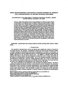
A data set is composed of a set of graphs, Γ. Each graph, Gj ∈ Γ, is assigned a “ground truth” label of positive if it contains the target concept and negative if it does not. The set of positive graphs is denoted G+ and the set of negative graphs is denoted G− . Each graph Gj contains some number of objects. We refer to the ith object of the j th graph as oji . Each object has a set of attributes. The learning problem to be solved is: given some number of positive and negative graphs, construct a model that can assess the probability that a given graph contains the target concept [8]. Each graph is classified as either positive or negative on the basis of whether or not some subset of its objects matches the target concept definition. For instance, a target concept may be “a red object near a green object.” When, for example, blue objects are also present in some of the positive graphs, the learning approach must weigh the set of possible target concepts, and choose the one that best explains the positive graphs. This problem of having to identify the subset of objects and their relationships that define a target concept can be viewed as one of multiple instance learning (MIL) [9], [10], [11], [8]. III. SMRF T REES Figure 1(a) illustrates an example SMRF tree that identifies “yellow” objects. The first node dynamically binds some object from the graph to the variable A. This instantiation action enables SMRF trees to classify graphs based on attributes of particular objects or of relations between sets of objects. The question in the figure has been rendered in English, however the question is actually asked with respect to the color represented as a 3-vector (RGB). Specifically, the color of the object is compared with a decision volume in the RGB space. The answer to the question is “yes” if the object’s color property falls inside this volume, “no” if not, and “error” if the object has no color attribute. The leaf nodes represent a probability function over membership in the target concept. In this example, “yellow” objects are the most likely examples of the target concept. When this tree is used to classify the set of objects shown in Figure 1(c), A is instantiated with each object in turn. Here, objects 1 and 4 fall into the “Yes” leaf and are assigned a probability of 98% of being in the target concept. Such a probability would arise during the training process when a vast majority (but not all) of the examples arriving at this node are labeled as positive examples of the target concept. Objects 2, 3 and 5 are sorted into the “No” leaf. The SMRF tree is capable of asking questions with respect to the properties of multiple objects and relations. A more complicated example tree is given in Figure 1(b). This tree identifies a “yellow object that is near a red object.” As before, A is instantiated with each object in turn. When A = 1 or A = 4, B is instantiated with a second object drawn from the graph. The SMRF tree then asks whether B is “red” by examining another color model. If this is the case, the final

Figure 1. (a) A hand-crafted SMRF tree that identifies yellow objects. Although we describe the decision tree split with a categorical label (“yellow”), the concept is represented as a volume in RGB space. (b) A tree that identifies yellow objects that are near red objects. (c) A set of objects scattered on a plane.

question examines the relative position of A and B. In this example, the position of A is measured within a coordinate frame whose origin is defined by the position of object B. We refer to a specific ordered list of instantiations (e.g., A = 1 and B = 2) as an instantiation sequence. The variables are implicit in the order of the sequence. For example, the set of instantiation sequences that is expanded by the tree in Figure 1(b) for the objects in Figure 1(c) is: • leaf 1: {(2), (3), (5)}, • leaf 3: {(1, 2), (1, 4), (4, 2), (4, 1)}, • leaf 5: {(4, 3)}, and • leaf 6: {(1, 3), (1, 5), (4, 5)} . Formally, for a given graph Gj and edge e in the tree, we refer to ith instantiation sequence as e Iij . The set of all instantiation sequences at edge e and graph Gj is e I j , and the set of all instantiation sequences at edge e for all graphs is e I. It is also convenient to refer to the set of instantiation sequences that arrive at a node in the tree from its parent

edge. For example, we refer to q I as the set that arrives to question node q and k I as the set that arrives at leaf k. Each node in a SMRF tree performs specific operations on the set of instantiation sequences. These operations are described in the following sections. Root Node. The root node, represented by a triangle in Figure 1(a,b), is the point in the tree at which no instantiations have been performed. Hence, this node has no parent edge and a single child edge. For each graph Gj , the root node induces a single instantiation sequence on the child edge. Specifically, 0 I j = {()}. Instantiation Nodes. Instantiation nodes assign a new object to each instantiation sequence. Specifically, for each instantiation sequence arriving from the parent edge, all possible non-duplicate objects from the graph are appended to the sequence: c j

I =

[

[

I∈p I j

o∈(Gj −I)

A PPEND(I, o),

where p I j is the set of instantiation sequences arriving at the parent edge of the instantiation node for graph Gj , c I j is the set of corresponding instantiation sequences at the child edge of the instantiation node, and A PPEND(I, o) adds new object o to the end of the sequence of objects encoded by I. The set of objects (Gj − I) are those in graph Gj that have not been instantiated in I. Note that each instantiation sequence at the parent p Iij gives rise to a set of instantiation sequences. We denote this set of child instantiation sequences with c Iij ⊂ c I j . Question Nodes. Question nodes sort instantiation sequences arriving at the parent edge into one of several child edges as a function of the attributes of the objects contained within the instantiation sequence and their associated relations. It is possible to capture this decision volume in many ways. Here, we represent the question at node q as a probability density function (pdf) defined over I (designated by model Mq ) and a threshold. Specifically, if p(I|Mq ) ≥ Θq , then I is sorted into the Yes child edge. If p(I|Mq ) < Θq , I, is sorted into the No edge. Model Mq defines: 1) a function, called a mapping function, that maps the attributes of the objects contained by I into a metric space 2) a pdf over the metric space, and 3) the parameters of the pdf. Mapping functions can map any combination of attributes from any combination of objects in I into a metric space, providing a wealth of possibilities. For example, a mapping function could capture the position of an object relative to another object, the position of an object relative to a coordinate frame defined by several other objects, or the relative color of two objects. In the case that a mapping function references an attribute that is not defined by some object, the instantiation sequence cannot be properly evaluated. In this case, the instantiation

sequence is sorted into the Error edge. The Error edge is considered a normal edge of the tree. Leaf Nodes. We denote the set of leaves for a given tree with L. We refer to instantiation sequences that arrive at some leaf as complete instantiation sequences. The set of complete instantiation sequences that arrives at leaf k ∈ L is denoted k I, and the set of all complete instantiation sequences is L I. Instantiation sequences sorted into leaf k are assigned a probability P r(k) of encoding the target concept. L(I) denotes a function that maps a complete instantiation sequence I ∈ L I to the leaf to which it is sorted. P r(L(I)) denotes the probability that complete instantiation sequence I encodes the target concept. Graph Evaluation. The SMRF tree assesses the probability that a given graph contains the target concept. A graph Gj is evaluated by first identifying the set of complete instantiations, L I j . The highest probability complete instantiation sequence determines the probability of the entire graph. Specifically: P r(Gj contains the target concept) = max P r(L(I)). I∈L I j

IV. L EARNING A LGORITHM The objective of the SMRF tree learning algorithm is to grow a tree that can accurately predict whether or not a particular graph contains the target concept. For the purposes of generality, we assume that the information that is provided at the time of training does not identify the key objects or their associated properties. The tree learning problem can therefore be seen as an instance of the multiple instance learning problem [9], [10], [11], [8]. Each set of complete instantiation sequences, L I j , is a bag that is labeled as either containing an example of the target concept (a positive bag) or not (a negative bag). The challenge is to identify the target concept that, if found within a bag, results in the bag as being labeled as a positive example. In our context, if the bag is a positive example, then we expect the tree to assign a high probability of being in the target concept to at least one complete instantiation sequence. The remaining instances are assumed to not be examples of the target concept, and thus should be assigned a low probability. If the bag is labeled as being a negative example, then all complete instantiation sequences are considered to be negative examples of the target concept. The challenge in growing the tree is one of improving the sorting of positive complete instantiation sequences from negative ones. However, we do not know a priori which complete instantiation sequences are the positive or negative examples of the target concept. Following Zhang & Goldman (2001) [11], we address this question by introducing a set of hidden variables that represent the probability that each instantiation sequence corresponds to an example of the target concept. Specifically, for each instantiation sequence,

e j Ii ,

there exists a variable, denoted h(e Iij ), that captures this probability. Since negative bags cannot contain the target concept, no instantiation sequences from a negative graph can ever match the target concept. Thus, h(e Iij ) = 0 for all instantiation sequences associated with negative graphs. On the other hand, we assume that a positive bag contains 1 one example P of the target concept. Specifically, for every Gj ∈ G+ , I∈L I j h(I) = 1. The process of learning a SMRF tree from a given set of labeled example graphs is performed incrementally. This process involves two key components. The lowest level component, question optimization (described in Section IV-A) is responsible for the selection of model parameters, hidden variables and leaf probabilities given a specific model and mapping function. The highest level component, tree growth (Section IV-B) is responsible for first selecting the candidate leaf nodes for possible expansion and identifying the particular form of expansion, including selection of the question models and mapping functions. Following the question optimization step for each of these candidates, this high-level component is responsible for deciding whether the tree should be expanded, and if so, which of the candidate expansions to keep. A. Question Optimization Given that the type of question and the mapping function have already been chosen, we employ an iterative algorithm that simultaneously estimates the hidden variable states (the h(I)’s) and the various model parameters (P r(k)’s and the parameters of Mq ). An outline of the algorithm is given in Section IV-C (see OptimizeQuestion). Selecting Question Parameters. Assuming known h(I)’s for a set of instantiation sequences, q I, the goal is to select model parameters for question node q that will sort instantiation sequences with high h from those with low h. We do this by first computing the weighted maximum likelihood parameters for the model pdf, where the sample weights are determined by the associated h’s. Specifically, the weighted model likelihood is defined as follows: ˆ L(q) =

Y

p (I|Mq )h(I) .

(1)

I∈q I

The intuition is that instantiation sequences with higher h values should contribute the most to the selection of the parameters, whereas instantiation sequences with low h values should contribute little to nothing. The next step is to select the model threshold Θq that will determine which instantiation sequences will be sorted into the Yes/No edges of the tree. For the results reported in this paper, we choose a fixed likelihood threshold that corresponds to 4σ. This choice allows a high percentage 1 In the general MIL case, one assumes one or more instances of the target concept in each positive example.

of false negatives to be eliminated, without dramatically increasing the number of false positives. Estimating Leaf Node Probabilities. In typical probability trees, the probability associated with a leaf node can be estimated from a training set by counting. However, the true labels of the instantiation sequences are unknown. Instead, we employ “soft” counting. Formally, this is expressed as: X P r(k) ← h(I)/ k I . (2) I∈k I

Hidden Variable Estimation. Given that the question parameters have been estimated (and consequently the instantiation sequences have been sorted), and that the leaf node probabilities have also been estimated, the algorithm seeks to select a set of h’s that are consistent with the sorting. This is accomplished by maximizing the likelihood (L) of correct sorting: L=

Y

P r (L(I))

h(I)

(1 − P r (L(I)))

(1−h(I))

.

(3)

I∈L I

Solving for the h’s reduces to a linear programming problem in which log L is maximized subject to set of constraints. These constraints are: • for each I: 0 ≤ h(I) ≤ 1, − 0 j • for each Gj ∈ G and each I ∈ I : h(I) = 0, + 0 j • for each Gj ∈ G and each I ∈ I : h(I) = 1, and • for each instantiation sequence X arriving at an instantiation node, p Iij : h(p Iij ) = h(I). I∈c Iij

In the latter constraint, a parent instantiation sequence distributes it’s associated h across its children. As detailed in OptimizeQuestion, the h’s that are local to the question node are first selected to maximize (3) (along with the question node parameters and leaf node probabilities). Then, the h’s throughout the tree are reestimated. This process is repeated until a local maxima is reached. This hierarchical approach allows for a correct model to be learned at the question node, before the other models in the tree are adjusted to account for the new one. B. Tree Growth The tree growth process is responsible for identifying candidate leaf nodes to expand, selecting the type of expansion to perform, evaluating the consequences of the expansions and choosing which candidate to keep. In this section, we describe the key details. The algorithmic components are outlined in Section IV-C. Identifying Candidate Leaves for Expansion. At the beginning of any given iteration in the learning process (represented by a call to G ROW T REE in Section IV-C), the learning algorithm begins by choosing a set of candidate leaves for expansion. The algorithm first evaluates all leaves according to an inexpensive expansion criterion, and then

selects the best m for possible expansion. The expansion criterion is the expected increase in likelihood (Eq. 3) that would result by adding an “optimal” split between the Yes and No branches. Selecting Candidate Expansions. Once a leaf node has been selected for expansion, the details of the expansion must be determined. We first determine the structural form of the expansion, and then select the mapping function that will determine the question that is to be asked. The structural form of the expansion is determined by replacing the leaf node with a new sub-tree. The possible forms of this subtree are: •

• •

a question node (designated tq in algorithm E XPAND L EAF); an instantiation node, followed by a question node (tiq ); two instantiation nodes, followed by a question node (tiiq ).

In all cases, question nodes have child leaf nodes that correspond to the Yes, No and Error branches. The mapping function is sampled from a set of candidate mapping functions (within algorithm F IND B EST M ODEL). This set of mapping functions is determined by 1) the set of objects in the arriving instantiation sequences, 2) the attributes of these objects, and 3) the attributes of the relations between these objects. For example, a mapping function may describe the position of the second object in the instantiation sequence within a coordinate frame that is rooted at the first object and whose orientation is determined by the position of the third object relative to the first. Evaluating the Candidate Expansions. For each candidate expansion, the parameters of the question and leaf nodes, and the instantiation sequence probabilities (the h(I)’s) are selected as described in Section IV-A (algorithm OptimizeQuestion). When the candidate expansion includes an instantiation node, the set of initial h(I) values for the child instantiation sequences is sampled multiple times. For each of these samplings, OptimizeQuestion is performed. We maintain the best performing parameter set (with respect to L) for the candidate expansion. Over the set of candidate expansions, the best performing candidate tree, Tc , is considered as a replacement for the current tree. If this new tree performs significantly better than the current tree according to a likelihood ratio test, then this replacement is kept. Because the sample size is reasonably large, −2 log LLT is approximately χ2 distributed c with degrees of freedom equal to the difference in the number of parameters in the candidate tree and the current tree [12]. The number of parameters in the tree is the number of leaf nodes plus the sum of the number of distribution parameters in each question node. To compensate for the multiple comparisons we employ a Bonferroni correction to obtain a collective cutoff of α = 0.05 [13].

C. Algorithm Pseudocode G ROW T REE(T, Γ) for k ∈ LT compute expansion criterion for each leaf for m-best leaves, i = 1 to m Ti ← E XPAND L EAF(k, T, Γ) return Ti with highest significant LTi (Eq. 3) E XPAND L EAF(k, T, Γ) expansion types ← {tq , tiq , tiiq } for t ∈ expansion types replace leaf k in T by expansion type t, to make Tt let qt be the newly-created question node (LTt , Mqt ) ← F IND B EST M ODEL(Tt , qt ) set Mqt as the model of node qt return Tt with greatest LTt F IND B EST M ODEL(T, q) Lbest ← −∞; qbest ← N one F ← samples of the set of mapping functions for fm ∈ F H ← samples of the set of initial h(I) values for h ∈ H (Lh , qh ) ←O PTIMIZE Q UESTION(T, q, q I, fm , h) LBest ← maxh Lh ; qbest ← qh return (LBest , Mqbest ) O PTIMIZE Q UESTION(T, q,q I, fm , hinit ) h(q Iij ) ← hinit ; Lold ← −∞; Lnew ← LT while (Lnew − Lold ) > ǫ while (Lnew − Lold ) > ǫ ˆ choose params of Mq to maximize L(q) (Eq. 1) estimate leaf node probabilities (Eq. 2) estimate h’s local to q to maximize LT (Eq. 3) Lold ← Lnew ; Lnew ← LT computed with new h’s estimate all h’s to maximize LT (Eq. 3) Lold ← Lnew ; Lnew ← LT computed with new h’s return (Lnew , q) V. E XPERIMENTAL R ESULTS Our experimental goals are to show that the learning algorithm is able to 1) select the appropriate attributes and mapping functions from a range of possibilities, 2) create complex target concepts involving multiple questions, and 3) deal with the presence of “distractor” objects that do not play a role in the true target concept. We employed data sets involving objects with attributes of 2D position and RGB color. We chose the following target concepts for our experiments: • a red object above a green object, • a red object near a green object, and • an object to the left of a lighter-colored object.

Note that each target concept not only involves the creation of categories of individual attributes (greenness, for example) but also of relations between objects (nearness, relative location and relative brightness). We also varied the number of excess objects in each example by adding two and five distractor objects to the graphs. A number of different mapping functions were made available to the learning algorithm. The algorithm could choose to model the absolute location of an object in R2 , the Euclidean distance between two objects in R2 , or the difference vector between two objects in R2 . The pdfs used for these models were Gaussian distributions of 2, 1 and 2 dimensions, respectively. For the color attribute, the algorithm could choose to model either the RGB color of a single object, the Euclidean distance in RGB space between the colors of two objects, or the difference vector in RGB space between the colors of two objects. These pdfs were also Gaussians of 3, 1 and 3 dimensions. For each of the three data sets, 100 positive example graphs and 100 negative example graphs were generated using a set of hand-selected rules. We employed 10-fold cross-validation. For each of the 10 experiments, 90 examples of each type were used for training and the remaining 10 examples of each type were withheld for testing. In all cases, performance is reported in terms of these test sets. Because SMRF trees classify probabilistically, we measure classification performance in terms of the receiver operating characteristic (ROC) curve and the area under the curve (AUC). We performed a total of five separate experiments. The first three experiments correspond to the three target concepts in which no distractor objects were present in any of the examples (all objects in each example played a role in the target concept). The two remaining experiments correspond to the red above green target concept with two and five distractor objects in each example. These distractor objects played no role in the target concept. For the red near green experiment (zero distractors), the resulting trees tend to have structure similar to that shown in Figure 1(b). However, on average, the trees contain 4.4 question nodes, whereas the ideal tree contains only three nodes. Nevertheless, the mean AUC over the ten experiments is 0.92. The learned trees for the red above green experiments also perform well. As an example, the mean ROC curve for the 2 and 5-distractor cases are shown in Figure 2. The standard deviation of the curves is represented as a shaded area around the mean. The mean AUC for these two curves is 0.94 and 0.89, respectively. The results of all five experiments are summarized in Table I. This table shows the mean and standard deviation of the AUCs, the number of question nodes per tree, and the total relative instantiation sequence count (TRISC). The minimum number of question nodes that can represent the light on right target concept is two. The minimum number

(a) Red Above Green: 2 Distractors

(b) Red Above Green: 5 Distractors Figure 2. Mean ROC Curves over ten cross-validated experiments for the 2 and 5-distractor Red above Green experiments.

of question nodes for the remaining concepts is three. TRISC measures how well the SMRF algorithm avoids the combinatorial explosion of considering all orderings of objects in the examples, and is defined as: T RISC = |L I| /

X

|Gj |,

Gj ∈Γ

where smaller values approaching unity are better. The algorithm performs consistently across the nodistractor experiments. The only notable difference is that the light on right experiment requires on average more than one fewer question node, reflecting the fact that this target concept requires one less node in the ideal case. The ideal TRISC of unity of these experiments is due to the fact that with no distractors, there can never be more complete instantiation sequences than objects regardless of the number of

Table I SMRF C LASSIFICATION P ERFORMANCE Target R near G Light on Rt R above G

Distractors 0 0 0 2 5

AUC 0.92 ± .050 0.96 ± .036 0.92 ± .071 0.94 ± .040 0.89 ± .090

Num. 4.4 ± 3.0 ± 4.5 ± 3.1 ± 3.6 ±

Qs 0.9 1.2 0.7 0.3 .91

R EFERENCES TRISC 1.0 ± 0.0 1.0 ± 0.0 1.0 ± 0.0 1.4 ± 0.06 1.7 ± 0.23

Learning algorithm performance on five problems. For each problem, we report the mean and standard deviation over ten cross-validated experiments of the Area Under the Curve (AUC), number of question nodes in the learned tree and the Total Relative Instantiation Sequence Count (TRISC).

instantiation nodes. As the number of distractors increases, the average AUC does not drop substantially. The TRISC metric does show an increase as the number of distractors increases. However, this increase is substantially smaller than the polynomial growth that is expected in the worst case. This indicates that the learned trees tend to sort many of the instantiation sequences into shallow branches. VI. D ISCUSSION AND C ONCLUSION The SMRF tree learning algorithm must simultaneously identify the objects contained within the training set graphs that participate in the target concept, along with the set of object and relational attributes that explain the target concept. The algorithm performs well for the synthetic tasks reported in this paper. Given the preliminary status of the SMRF tree algorithm implementation, we feel that these results indicate that this learning approach has a great deal of promise. We are currently pursuing experiments in which a robot must learn to distinguish the goal configuration of a stacked set of objects from other presented configurations. This capability will serve as the basis for the robot to learn how to complete a task given the current configuration of a set of objects. Much work still remains to be done to realize a full implementation of the SMRF tree approach. Future components will focus on incorporating temporal attributes and relations into the learning algorithm. In addition, we plan to add the ability for SMRF trees to make predictions about the unobserved attributes of an object or its relations. This step will, for example, allow a SMRF tree to predict the future location of an object with respect to other objects in the graph. We plan to demonstrate the utility of this learning approach in variety of domains, including the learning of robotic manipulation sequences from demonstration by a human teacher, and the prediction of the likely touch-down region of tornadoes. ACKNOWLEDGMENT This material is based upon work supported by the National Science Foundation under Grant Nos. IIS/REU/0755462 and IIS/CAREER/0746816.

[1] J. Neville, D. Jensen, L. Friedland, and M. Hay, “Learning relational probability trees,” in Proceedings of the Ninth ACM SIGKDD International Conference on Knowledge Discovery and Data Mining, 2003, pp. 625–630. [2] A. McGovern, N. Hiers, M. Collier, D. J. Gagne II, and R. A. Brown, “Spatiotemporal relational probability trees,” in Proceedings of the 2008 IEEE International Conference on Data Mining, Pisa, Italy, December 2008, pp. 935–940. [3] J. Kubica, A. Moore, and J. Schneider, “Tractable group detection on large link data sets,” in The Third IEEE International Conference on Data Mining, X. Wu, A. Tuzhilin, and J. Shavlik, Eds. IEEE Computer Society, 2003, pp. 573–576. [4] J. Kubica, A. Moore, D. Cohn, and J. Schneider, “Finding underlying connections: A fast graph-based method for link analysis and collaboration queries,” in Proceedings of the International Conference on Machine Learning, 2003, pp. 392–399. [5] D. Jensen and L. Getoor, “IJCAI 2003 workshop on learning statistical models from relational data,” 2003, http://kdl.cs.umass.edu/srl2003/. [6] N. Friedman, L. Getoor, D. Koller, and A. Pfeffer, “Learning probabilistic relational models,” in Proceedings of the International Joint Conference on Artificial Intelligence, 1999, pp. 1300–1309. [7] L. Getoor, N. Friedman, D. Koller, and B. Taskar, “Learning probabilistic models of link structure,” Journal of Machine Learning Research, vol. 3, pp. 679–707, 2002. [8] A. McGovern and D. Jensen, “Identifying predictive structures in relational data using multiple instance learning,” in Proceedings of the 20th International Conference on Machine Learning, 2003, pp. 528–535. [9] T. G. Dietterich, R. H. Lathrop, and T. Lozano-Perez, “Solving the multiple-instance problem with axis-parallel rectangles,” Artificial Intelligence, vol. 89, no. 1-2, pp. 31–71, 1997. [10] O. Maron and T. Lozano-P´erez, “A framework for multipleinstance learning,” in Advances in Neural Information Processing Systems 10, M. I. Jordan, M. J. Kearns, and S. A. Solla, Eds. Cambridge, Massachusetts: MIT Press, 1998, pp. 570–576. [11] Q. Zhang and S. Goldman, “EM-DD: An improved multipleinstance learning technique,” in Proceedings of Neural Information Processing Systems, vol. 14. MIT Press, 2001, pp. 1073–1080. [12] J. P. Huelsenbeck and K. A. Crandall, “Phylogeny estimation and hypothesis testing using maximum likelihood,” Annual Review of Ecology and Systematics, vol. 28, pp. 437–466, 1997. [13] D. Jensen and P. Cohen, “Multiple comparisons in induction algorithms,” Machine Learning, vol. 38, no. 3, pp. 309–338, 2000.