Spatiotemporal Relational Probability Trees: An Introduction Amy McGovern University of Oklahoma
[email protected] Matthew Collier University of Oklahoma
[email protected]
Nathan C. Hiers Atmospheric Technology Services Company
[email protected]
David J. Gagne II University of Oklahoma
[email protected]
Rodger A. Brown NOAA/National Severe Storms Lab
[email protected]
Abstract We introduce spatiotemporal relational probability trees (SRPTs), probability estimation trees for relational data that can vary in both space and time. The SRPT algorithm addresses the exponential increase in search complexity through sampling. We validate the SRPT using a simulated data set and we empirically demonstrate the SRPT algorithm on two real-world data sets.
1
Introduction
The real world is composed of objects, such as people, places, and things, and relationships between the objects, such as events. Statistical relational learning, inductive logic programming, and relational knowledge discovery methods focus on learning in exactly this domain and have proven successful in many real-world examples (e.g., [3, 4, 10, 13]). However, these approaches either ignore the temporal aspect of the data or tailor an approach specific to the data set. The main contribution of this paper is a principled approach to learning in spatially and temporally varying relational data that directly addresses the difficulties inherent in both the conceptualization of the data and in learning the model. To our knowledge, [19] is the only other approach that directly models the temporal nature of relations (but not the objects or attributes) by employing a weighted graph scheme similar to [6]. This work is motivated by two real-world severe weather domains where we believe that spatiotemporal knowledge discovery methods can have a significant impact. On the smaller spatial and temporal scale, phenomena such as tornadoes, severe thunderstorms, hail, and flash floods annually cause significant loss of life, property, and societal disruption [16]. On the regional scale, drought, has one of the highest costs of any natural event in terms of socioeconomic
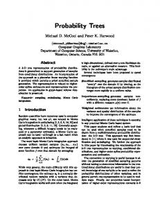
(a) 140 minutes
(b) 150 minutes
Figure 1. (a and b) The red area shows the region of strong updraft, the blue region shows the strong downdraft, and the green region shows the area of strong vertical vorticity.
loss [12]. Clearly, mitigating the effects of both types of severe weather would be beneficial. Figure 1 (a and b) show examples of the three dimensional meteorological fields that we use in our simulated supercell thunderstorms. The regions of strong updraft (air moving upward), downdraft (air moving toward the surface), and vertical vorticity (a measure of instantaneous rotation around a vertical axis) for a single storm are shown ten minutes apart. Although defining the exact dynamics of the regions is difficult, it is clear that the storm has evolved significantly in both space and time. For example, the storm has developed two distinct regions of vertical vorticity reaching to the ground and the downdraft has also grown and begun to wrap around the updraft. Our long term goal is to enable domain scientists to better understand the evolution of severe weather by creating human readable models that can mine large spatiotemporal data sets. In this paper, we specifically focus on classification tasks motivated by severe thunderstorms and tornadoes and we are currently examining the application to drought.
The Spatiotemporal Relational Probability Tree (SRPT) is a probability estimation tree that learns with spatiotemporal relational data. For example, a SRPT can predict new class labels based on questions such as “Has a downdraft lasted for at least 5 minutes?” or “Did a region of strong tilting of horizontal vorticity appear before the downdraft doubled in intensity?” While the SRPT was inspired by the the relational probability tree (RPT) [14], the SRPT represents both the data and the decision tree distinctions in a very different manner.
2
Spatiotemporal Relational Data
An efficient representation for spatially and temporally varying data has been the subject of research in the field of geographic information science [7]. We use a combination of the span approach [5] and the attributed graph [13]. In our approach, a graph, G, is represented by G = (V, E, A(V ), A(E), T (V ), T (E)). Objects, such as updrafts or downdrafts, are represented as vertices (V) in the graph. Relations between these objects, such as Contains(updraft, downdraft), are represented by edges (E) between the objects. For a given relation r(o1 , o2 ), o1 , o2 ∈ V and r ∈ E. The key difference from standard static attributed graphs is that objects and relations can be either static or dynamic. If they are dynamic, they only exist for a period of time defined inside each object or relation (T (V ) and T (E) respectively). Attributes are associated with objects, A(V ), such as updraft.volume, or relations, A(E), such as Nearby.distance. Temporally varying attributes are represented as streams [15]. Objects and relations can also have static attributes and we assume that all objects and relations have a static type attribute.
3
Grow-SRPT(data, pvalue, # samples) 1. Root ← FindBestDistinction(data, pvalue, # samples) 2. (yes, no) ← partition data using Root’s distinction 3. For dataSubset in (yes, no) 4. node ← GrowSRPT(dataSubset, pvalue, # samples) 5. add node as a child of Root 6. Return Root FindBestDistinction(data, pvalue, # samples) 1. Loop # samples times 2. distinction ← obtain randomly sampled distinction 3. (chi, p) ← get χ2 and p-value for distinction 4. Return distinction with best χ2 such that p < pvalue. If no such distinction exists, return Leaf. Table 1. Pseudocode for learning an SRPT ple from the data itself to fill in the missing values. For example, if we randomly chose an attribute distinction, we would randomly pick an object type (e.g. updraft), an attribute (e.g. maximum strength), a split type (e.g. ≥), and a value (e.g. 35 m/s). This would yield a distinction that splits the data by asking “Is there an updraft whose maximum updraft speed reaches at least 35 m/s?” The primary difference between an SRPT and other decision trees and specifically from RPTs is the set of distinctions that the SRPT can use. Classical decision trees primarily split the data based on questions such as “is attribute x ≥ y?” We expand the possible set of distinctions to include questions based on temporal and spatial variations. The current set of distinctions for the SRPT is given in Table 2. We are currently working on expanding the set of possible distinctions with a particular focus on spatial and spatiotemporal distinctions (e.g. [24]).
SRPT Algorithm 4
An SRPT is a probability estimation tree, which is a decision tree with class probabilities at the leaf nodes. The SRPT learning algorithm follows the standard decision tree algorithms with one exception, detailed below. Table 1 gives pseudocode for learning an SRPT given training data. The exception is that we uniformly sample distinctions instead of examining all possible distinctions. This occurs in FindBestDistinction. Relational spaces already have a large search space and adding spatiotemporal features only compounds the problem. Srinivasan [21] demonstrated that we can find a distinction in the top p% of all distinctions with confidence of α by choosing a number of samples n (1−α) where n ≥ ln ln (1−p) . Critically, the number of samples does not depend on the size of the search space. We empirically examine the effect of sampling on the algorithm. To generate a randomly sampled distinction, we first randomly select a distinction type (listed below) and then sam-
Data sets
We examine the behavior of the SRPT algorithm in three data sets. The first is a synthetic domain where we know the correct answers and can explore the parameter space. The remaining domains are real-world problems. Shapes world: The first domain is a simulated world full of three dimensional shapes with temporal extent and temporally varying characteristics. There are three possible objects: balls, pyramids, and cubes. Each object has two attributes: a static attribute of color (red, green, blue) and a temporally varying attribute of volume. Each shape is randomly placed in at least one relationship with another shape (Nearby or OnTopOf). The relationships also have a distance attribute that varies temporally. Each graph contained between five and ten objects. We varied the volumes temporally either randomly, in an increasing manner, or a decreasing manner. A positive graph was defined as one
# 1 2 3
Distinction Exists Temporal Exists Attribute Value
Type Basic Basic Basic
4
Temporal Gradient
Basic
5 6 7
Count Structural Temporal Ordering
Conjugate Conjugate Conjugate
Description Does a object or relationship of type t appear in the graph? Is there is an object or relationship of a particular type that lasts at least t steps? During an object or relation of type t’s existence, was the (mean, median, maximum, minimum, or any) value of attribute a greater than or equal to value v? Is the partial derivative with respect to time of an attribute value a on an object or relation of type t greater than or equal to v? Is the number of matching items of basic distinction b at least v? Does the match from basic distinction b relate (type t) to an object (type p)? Do the matching items from basic distinction a occur in a temporal relationship with the matching items from basic distinction b? The seven types of temporal ordering are: before, meets, overlaps, equals, starts, finishes, and during [2].
Table 2. Types of distinctions the SRPT can choose from in building the trees. with at least three red balls whose volume is greater than 5 at some point. We generated 30 separate training and test set splits, each with 250 graphs and a 50/50 class distribution. Reality: The Reality Mining group at MIT1 collected data from the cell phones of nearly 100 people at MIT. Each cell phone recorded when it was in the vicinity of another cell phone, in use, near a tower, or near a bluetooth device. Based on the results in [20], we reduced the data to people, phone, and device objects and aggregated the temporal resolution to two weeks. The four class labels are student, faculty/staff, Sloan associate, and unknown. Simulated supercell thunderstorms: We apply the SRPT to 163 simulated four dimensional supercell thunderstorms each generated by varying appropriate environmental parameters [17]. We used the Advanced Regional Prediction System (ARPS), which is a three-dimensional, nonhydrostatic model that is one of the top systems for simulating thunderstorm data [23]. The model is run for three hours with history files saved every 30 seconds. Each storm simulation produces 20 GB of data and we have 6 TB of data which requires any method that we develop to work efficiently with large data sets. Simulated data provides us with a high resolution dynamically consistent field of meteorological quantities. Simulations have been used successfully to study severe weather including tornadoes (for example, see [8, 1]). By applying our data to a full meteorological field of variables, we expect to identify the critical interactions of meteorological quantities as they evolve in a severe storm. Each simulation can produce multiple severe storms which we identify and track individually using a modified form of the Storm Cell Identification and Tracking algorithm [9]. We focus on regions with strong updrafts as this is the key dynamic feature of a supercell. For each storm, we identify 16 different types of objects and 4 possible types of relationships among these objects (described in 1 http://reality.media.mit.edu/
Table 3). Each object and relationship has temporally varying attributes associated with it. The objects and attributes are drawn from the high level features that meteorologists currently use to study storms (e.g., [11, 18]). Because the 0.5 km horizontal resolution of our simulations is too coarse to detect a rotation on the scale of a tornado (and scaling the resolution appropriately requires exponentially more computational power and storage space), we label each storm as to whether it generated a strong lowaltitude rotation (“positive”), was ambigious (“maybe”), or clearly had no strong low-altitude rotations (“negative”). Positive storms were labeled (1) by finding pressure perturbations less than −1000 Pa (2) with at least 500 Pa drop within 5 minutes (3) that occur in the lowest 2 km of the atmosphere, (4) that overlap, contains, or equals a region with strong vertical vorticity. Maybe storms are ambiguous and may contain any three of these criteria but not all four. At most two criteria may be true for a negative storm. This yielded 24 positive storms, 99 maybe storms, and 1393 negative storms for a total of 1516 storms. Prior to learning an SRPT, we also removed all the pressure, positive vertical vorticity, and negative vertical vorticity objects because they were used to label the data.
5
Empirical Evidence
We are not aware of other algorithms designed to work on spatiotemporal relational data, making direct comparison to other approaches difficult. The RPTs are the closest algorithm but they are not able to handle temporal data unless the temporal streams are treated as set-valued attributes and the objects and relations are all treated as static objects. We chose to compare versions of the SRPT with various key components removed. For all experiments, we ran four different versions of the SRPT. The first used only the basic distinctions (numbers 1-4 above). The second used all the non-temporal distinctions (numbers 1, 3, 5, and 6). The
Objects
Object Attributes Relationships Relation Attributes
Updraft, Cyclonic Downdraft, Anticyclonic Downdraft, Positive/Negative Baroclinic Term, Pressure, Hail, Rain, Mesocylone, Mesoanticyclone, Positive/Negative Tilting Term, Positive/Negative Vertical Vorticity, Positive/Negative Stretching Term Max/Min, Mean, Median, Standard Deviation, Volume, Base, Ceiling, Thickness, Horizontal area, Buoyancy max/min/median/standard deviation/range, Percent Forward Contains, Equals, Overlaps, Nearby Percent Overlap
Table 3. Objects, relationships, and attributes extracted from the thunderstorm simulations. Shapes world increasing temporal attributes
Storms Reality
1
0.7
0.2
0.9 0.8
0.15
basic All but temporal ordering No temporal All
0.6
0.5 0.1
0.4 TSS
0.6 TSS
TSS
0.7
0.5
0.3 0.05
0.4
0.2 0.3
basic All but temporal ordering No temporal All
0.2 0.1 0 10
1
10
2
10 Number of samples
3
10
0
basic All but temporal ordering No temporal All
0.1
4
10
−0.05 1 10
2
3
10
10 Number of samples
(a) Shapes world
(b) Reality
4
10
0 0 10
1
10
2
10
3
10
4
10
Number of samples
(c) Severe Storms
Figure 2. Average TSS in each of the three domains as a function of sample size. third uses all distinctions except temporal ordering (numbers 1-6) and the last used all seven types of distinctions. Given the nature of our temporal data, we expect the best performance from the full SRPT algorithm and the worst from the subset with no temporal distinctions. Although the shapes world is a binary classification task, the remaining two tasks are multi-class. Rather than use the area under the curve which is designed for binary tasks, we use the true skill statistic (TSS) [22]. This statistic is very similar to the area under the curve except that it varies from -1 to 1 with 0 being the performance of a random classifier. A TSS value of 1 is perfect.2
5.1
Shapes World: sensitivity testing
To assess the effect of sampling on the algorithm, we compared the average TSS of the SRPT as a function of the number of samples for each of the four sets of distinctions. Figure 2a shows the results of this comparison for the temporally increasing attributes. Due to space limitations, we do not show the results for the decreasing and random shape worlds but they are very similar. We averaged the TSS over 30 runs for each of the three test sets and we varied the sample size from 2 to 9209 by varying p from 0.9 to 0.0005 with a α of 0.99. At all sample values, the SRPT with all distinctions was statistically indistinguishable from 2 http://www.bom.gov.au/bmrc/wefor/staff/eee/verif/verif
web page.html
the SRPT without the temporal ordering distinctions and, at the higher sample values, both are better than the basic and non-temporal subsets of distinctions (p < 0.01). It is not surprising that temporal ordering is not useful in this task since it is not used in creating the simulated data. Likewise, it is not surprising that the non-temporal distinctions and the basic distinctions are unable to fully express the correct tree for any number of samples as the full answer requires counting. We also examined the effect of varying the statistical significance threshold with the expectation that higher p-values would create larger trees with lower predictive power. For this experiment, we varied both the p-value, the number of samples, and the set of distinctions available to the tree. The results were surprising in two ways. First, the tree size hypothesis, as measured by the number of leaves, was validated with larger p-values yielding significantly larger trees across all levels of sampling but only for the SRPT with the basic and the non-temporal distinctions. For the cases with all distinctions and with all but the temporal ordering, the size of the tree increased as a function of p-value only for small numbers of samples. With more samples, these trees were able to identify the critical conjunctive concepts necessary to describe the data and the trees were compact, regardless of p-value. Second, the quality of the trees, as measured by TSS, did not change appreciably as a function of tree size. The most likely reason for this is found in our tree growing algorithm. At each level of the tree, the dis-
2
20
21 10 3
41
7
1
32 24
erm gt
m str
etc
hin
m
ter tilt
ing
ter
ic lin
roc
ba
dra
cy clo
ne 2
so
ft
5
me
ft
wn do
dra
n
up
rai
il ha
13
1
exists
13
1
temporal exists
7
10
1
8
partial derivative
48
7
count conjunctive
attribute
structural conjunctive 5
8
54 14
5 8
9
8
78 62
3
72 27
temporal ordering Total
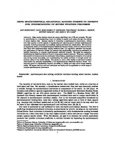
Figure 3. Frequency of object type and distinction type for all nodes in the trees across 30 runs of cross validation in the thunderstorm data.
tinction with the highest χ2 value was chosen so long as its p-value fell below the user’s specified threshold. Although higher p-values allow deeper trees to be created by overfitting to the noise in the data, at the higher levels of the trees, the same distinctions are likely to be found regardless of the user’s statistical significance threshold.
5.2
Reality
Figure 2b shows the average TSS as a function of sample size for the reality data. At the highest number of samples, the SRPT with all distinctions and with all but the temporal ordering distinctions is able to achieve an average TSS of 0.2. These numbers are averaged across 30 runs of 10 fold cross validation. The basic and non-temporal versions of the SRPT are never able to achieve a TSS greater than random. In most cases, particularly with the non-temporal version of the SRPT, the tree is unable to identify any significant distinctions and thus predicts the default label. Although an average TSS of 0.2 is not exceptionally high, it is clearly identifying useful structure in the domain.
5.3
Strong low-altitude rotations
As with the shapes world, we examine the performance of the SRPT algorithm using the three subsets of possible distinctions and with all distinctions as a function of sample size. Figure 2c shows the average TSS across 30 runs. As expected, performance improves as the number of samples
increases. Given the high performance at the highest levels of sampling, the trees themselves become the key result. The distribution of object types and distinctions identified throughout 30 runs of 2-fold cross validation is shown in Figure 3. The term mesocyclone indicates the presence of a rotating updraft. The baroclinic term, tilting term, and stretching term are terms in a theoretical equation that leads to vertical vorticity or local rotation about a vertical axis. Initially horizontal vorticity (local rotation about a horizontal axis) is present near the ground owing to the increase of wind speed with height in the lowest kilometer. Once the tilting term tilts horizontal vorticity into the vertical, the stretching term acts to concentrate the vorticity – increasing the strength of the mesocyclone. Though the process is not well understood, the intensification of low-altitude rotation appears to be associated with the formation of a localized downdraft on the back side of the rotating updraft (see Figure 1). All of the processes that play important roles in the initiation and intensification of rotation [11, 18], and especially low-altitude rotation, are prominently portrayed in Figure 3. Another distinction of severe thunderstorms is the presence of hail and that also is found to be an important object type in the tree.
6
Discussion
We have introduced a novel algorithm for identifying salient structure in spatiotemporal relational data and validated it on three disparate data sets. The performance of the SRPT with the thunderstorm data provides evidence towards the usefulness of the algorithm for complex realworld spatiotemporal data sets. The success with three data sets, each of which is very different from the others, indicates that the SRPT is versatile and will likely be useful for a wide variety of spatiotemporal relational data sets. The SRPT currently focuses its distinctions on the temporal nature of the data rather than the spatial nature of the data. The spatial distinctions arise from the spatial relationships define in the data. For example, the thunderstorm data defines the relative location of three dimensional regions using nearby, overlaps, equals, and contains. The SRPT can identify the critical relations and temporal variations of the attributes on each relation but it cannot currently identify spatial or spatiotemporal variations such as the increase in positive tilting as a function of altitude (and possibly time) or an updraft that starts nearby a downdraft but transitions to overlapping. In current work, we are expanding the set of distinctions to include additional spatial and spatiotemporal variations such as these. The work presented here is a first step along a path of more complex spatiotemporal relational models. Within the SRPT, we are working on expanding the types of possible distinctions based on the needs presented by both drought
and severe thunderstorm data. We are also exploring the effects of spatial and temporal autocorrelation on the models learned in these domains. Our thunderstorm simulations are limited by current computing power. We are preparing to study higher resolution data but this requires exponential increases in both computing power and storage space. We also plan to apply our techniques to assimilated data sets generated from actual storm observations as such data sets become available. Research Reproducibility The SRPT code and shapes world data is available at http://idea.cs.ou.edu/. The ARPS simulations are available by request (6TB of data). Acknowledgments This material is based upon work supported by the National Science Foundation under Grant No. NSF/IIS/0746816, NSF/CISE/REU 0453545 a seed grant from the University of Oklahoma’s College of Engineering, the Oklahoma Space Grant, and NASA Grant number NNG05GN42H.
[11]
[12]
[13]
[14]
[15]
References [16] [1] E. Adlerman and K. K. Droegemeier. The dependence of numerically simulated cyclic mesocyclogenesis upon environmental vertical wind shear. Monthly Weather Review, 133:3595–3623, 2005. [2] J. F. Allen. Time and time again: The many ways to represent time. International Journal of Intelligent Systems, 6(4):341–355, 1991. [3] S. Dzeroski and N. Lavrac, editors. Relational Data Mining. Springer, Berlin, 2001. [4] L. Getoor, N. Friedman, D. Koller, and B. Taskar. Learning probabilistic models of link structure. Journal of Machine Learning Research, 3:679–707, 2002. [5] P. Grenon and B. Smith. Snap and span: Towards dynamic spatial ontology. Spatial Cognition and Computation, 4(1):69–104, 2004. [6] S. Hill, D. Agarwal, R. Bell, and C. Volinsky. Building an effective representation for dynamic networks. Journal of Computational and Graphical Statistics, 15(3):584–608, 2006. [7] K. S. Hornsby and M. Yuan, editors. Understanding Dynamics of Geographic Domains. CRC Press, 2008. [8] M. Hu, M. Xue, K. Brewster, and J. Gao. Prediction of Fort Worth tornadic thunderstorms using 3DVAR and cloud analysis with WSR-88D Level-II data. In 11th Conference on Aviation, Range, Aerospace and 22nd Conference on Severe Local Storms, pages Electronically published, Paper J1.2, 2004. [9] J. T. Johnson, P. L. MacKeen, A. Witt, E. D. Mitchell, G. J. Stumpf, M. D. Eilts, and K. W. Thomas. The storm cell identification and tracking algorithm: An enhanced WSR88D algorithm. Weather and Forecasting, 13(2):263–276, 1998. [10] J. Kubica, A. Moore, and J. Schneider. Tractable group detection on large link data sets. In X. Wu, A. Tuzhilin, and
[17]
[18]
[19]
[20]
[21]
[22] [23]
[24]
J. Shavlik, editors, The Third IEEE International Conference on Data Mining, pages 573–576. IEEE Computer Society, 2003. L. R. Lemon and C. A. Doswell, III. Severe thunderstorm evolution and mesocyclone structure as related to tornadogenesis. Monthly Weather Review, 107:1184–1197, 1979. N. Lott and T. Ross. Tracking and evaluating U.S. billion dollar weather disasters. In Preprints of the 86th Annual Meeting of the American Meteorological Society, Atlanta, GA, 2006. A. McGovern, L. Friedland, M. Hay, B. Gallagher, A. Fast, J. Neville, and D. Jensen. Exploiting relational structure to understand publication patterns in high-energy physics. SIGKDD Explorations, 5(2):165–172, 2004. Winning entry to the open task for KDD Cup 2003. J. Neville, D. Jensen, L. Friedland, and M. Hay. Learning relational probability trees. In Proceedings of the Ninth ACM SIGKDD International Conference on Knowledge Discovery and Data Mining, pages 625–630, 2003. T. Oates and P. R. Cohen. Searching for structure in multiple streams of data. In Proceedings of the Thirteenth International Conference on Machine Learning, pages 346–354. Morgan Kaufmann, 1996. R. Pielke and R. Carbone. Weather impacts, forecasts, and policy. Bulletin of the American Meteorological Society, 83:393–403, 2002. D. H. Rosendahl. Identifying precursors to strong lowlevel rotation within numerically simulated supercell thunderstorms: A data mining approach. Master’s thesis, University of Oklahoma, 2008. R. Rotunno. Supercell thunderstorm modeling and theory. In The Tornado: Its Structure, Dynamics, Prediction, and Hazards, number 79 in Geophysical Monograph. American Geophysical Union, 1993. U. Sharan and J. Neville. Exploiting time-varying relationships in statistical relational models. In Proceedings of the 1st SNA-KDD Workshop, 13th ACM SIGKDD Conference on Knowledge Discovery and Data Mining, 2007. U. Sharan and J. Neville. Temporal-relational classifiers for prediction in evolving domains. In Proceedings of the IEEE International Conference on Data Mining, 2008. A. Srinivasan. A study of two probabilistic methods for searching large spaces with ILP. Data Mining and Knowledge Discovery, 3(1):95–123, 1999. D. S. Wilks. Statistical Methods in the Atmospheric Sciences. Academic Press, 2006. M. Xue, D. Wang, J. Gao, K. Brewster, and K. K. Droegemeier. The Advanced Regional Prediction System (ARPS), storm-scale numerical weather prediction and data assimilation. Meteorology and Atmospheric Physics, 82:139–170, 2003. M. Yuan and J. McIntosh. A typology of spatiotemporal information queries. In K. Shaw, R. Ladner, and M. Abdelgeurfi, editors, Mining Spatiotemporal Information Systems, pages 63–82. Kluwer Academic Publishers, 2002.