the success rate of correct unwrapping. Here, the mathematical framework for 3D spatio-temporal phase unwrapping using integer-least squares is presented.
SPATIO-TEMPORAL PHASE UNWRAPPING USING INTEGER LEAST-SQUARES ����
Freek J. van Leijen
����
, Ramon F. Hanssen
����
, Petar S. Marinkovic
�� �
, Bert M. Kampes
(1) Delft Institute of Earth Observation and Space Systems (DEOS), Delft University of Technology, Kluyverweg 1, 2629 HS Delft, The Netherlands (2) German Aerospace Center (DLR)–Oberpfaffenhofen, Remote Sensing Technology Institute, M¨unchner Strasse 20, 82234 Wessling, Germany
ABSTRACT State-of-the-art phase unwrapping techniques for interferometric time series do not fully benefit from the spatio-temporal correlations between the phase observations. Incorporation of these correlations in the unwrapping process may increase the success rate of correct unwrapping. Here, the mathematical framework for 3D spatio-temporal phase unwrapping using integer-least squares is presented. The technique is based on the 1D (temporal unwrapping) + 2D (spatial unwrapping) approach, currently applied in most Persistent Scatterer Interferometry (PSI) algorithms. The stochastic structures as well as the functional models are shown. 1 INTRODUCTION With the growth of the data archives, interferometric radar applications for deformation monitoring shifted from single interferogram to time series analysis. Examples of the latter are the Persistent Scatterer technique (PSI) [1, 2] and the optimal subsets approaches, e.g., [3, 4, 5]. Within the PSI technique the deformation of isolated point scatterers with stable phase behavior is estimated using a single master stack. On the other hand, the optimal subsets approaches use multi-looked interferograms with favorable baseline characteristics, grouped in subsets, to extract the deformation signal. Regardless the technique chosen, correct phase unwrapping remains the crucial step for a reliable analysis. So far, two main strategies for the unwrapping of the time series can be distinguished: 1) � 2D unwrapping using conventional techniques, e.g., [3, 4], and 2) 1D+2D unwrapping, e.g., [2, 5]. Obviously, unwrapping in multiple steps is suboptimal, as spatial and temporal correlations are not optimally taken into account. Here, the mathematical framework for an integrated 3D phase unwrapping algorithm is presented, based on the 1D+2D approach, which is discussed first. 2 1D+2D UNWRAPPING Within the 1D+2D approach, the time series of individual resolution cells are first independently unwrapped in time, followed by a spatial unwrapping step. To reduce the effect of atmospheric distortions in the temporal unwrapping step, often the differential phases between two nearby resolution cells are analyzed. These differential phases are denoted as double differences (DD), differences in time and space. The original interferometric phases are regarded as single differences (SD). 2.1 Temporal unwrapping Various temporal phase unwrapping techniques are proposed, each with their own optimization criterion and stochastic characteristics. Examples are the ambiguity function [6, 1], integer bootstrapping, and integer least-squares [7, 8]. The ambiguity function searches a discrete solution space for maximal temporal coherence, assuming a predefined functional model under the null-hypothesis (e.g. linear deformation). Because no stochastic properties of the phases are considered, the ambiguity function is a deterministic estimator. Using the integer bootstrapping technique, some of the correlation between the observations is taken into account. This implies that the stochastic model, describing the stochastic properties of the observations, needs to be known. An advantage of bootstrapping is that additional deformation parameters can easily be added. However, with the extra parameters the strength of the mathematical model is further reduced. The same holds for the integer least-squares (ILS) technique. However, here the full stochastic model is considered. For Gaussian distributed data, ILS is shown to be equivalent to the Maximum Likelihood estimator [9]. Because of this property and the large flexibility in deformation models that can be considered, the integer least-squares technique is applied here. The basic concept of the integer least-squares technique is to acknowledge the fact that some parameters, in this case the
ambiguities, are integer valued. The ILS problem can be denoted by the extended Gauss-Markov model as
�������� �� ������������ � �������
(1)
and the least-squares estimations are obtained solving the minimization problem
��"�#�!$�% �'&( ��&)�*� %,-/+ . �0�21�34�5�61879�:�;1=?� is the expectation operator, ���>=?� the dispersion, � the vector of phase observations, and � are design where � � � � is the covariance matrix. The matrices for the integer and real valued parameter vectors and respectively, and minimization problem Eq. (2) is solved in a three step procedure. First, the float solution is computed by neglecting � � the integer property of the ambiguities. Hence, a standard least-squares adjustment is applied to obtain the estimates @ , @ and A the accompanying variance matrix �CB � B $B = B D � $B " " B � " $E (3) Then, the ambiguities are resolved in a least-squares sense. To reduce the computation time, the ambiguities are ’decorrelated’ using the LAMBDA method (Least-squares AMBiguity Decorrelation Adjustment method)[7, 10]. The decorrelating transformation reads (4)
F @ ��G�H I� @ �
��J B ��G HK�C" B G�=
The integer ambiguities are obtained by solving the minimization problem
��J�MO�LN;P F @ & F>Q H *� JRTB S P F @ & FUQ = � Back-transformation yields the fixed ambiguities V .
(5)
�@
Once the ambiguities are estimated, the float solution of the parameters of interest is updated using the fixed ambiguities. The fixed solution reads
X�@ &'�*$B " B � "RYB S ��@ & � V Q � = �ZV � �*$B &(�*$B " B ��"RYB P S � " B $B \�*$B " B �*"RYB S � � " [ �^] F &)� Q F &(� Q H/_ �*V � P P J�MON P
��@ W " � �*$[ �
where
(6)
" [ �*"RYB S � " B $B � F>Q =
(7) (8)
� �`� Q _ � PV
Hence, the variance of the fixed solution is not only dependent on the variance of the float solution, but also on the chance of success in the ambiguity resolution. This chance of success is denoted by the success rate . Because of their discrete nature, the fixed ambiguities have a probability mass function (PMF) and the fixed solution a multi-modal probability density function. Unfortunately, the success rate for the integer least-squares estimator can not be computed in closed form. Therefore, simulations based on the mathematical model are required to estimate the success rate.
�V
�9� a A � d ga fb a � aTa;c b D e
Stochastic model for PSI The covariance matrix for the double difference phase observations are derived from the original Single Look Complex (SLC) observations by error propagation. The SLC observations are denoted as
jagc�i kml �n� oC���qpsr:tu \�qv5wyx;rX \�qz|{~}?r� (9) � indicate the points, is the number of SLCs (the master image is denoted by a zero), � z|{~}?r is the covariance where � v5wyx;r describes the variability of the atmosphere and � psr5t represents matrix due to residual (non-modeled) deformation, ha�ib
� ���
agcf
�����
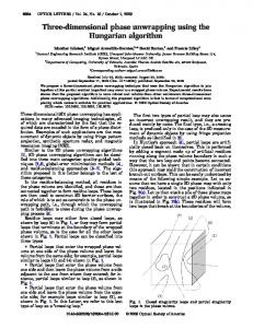
the noise due to loss of coherence and, e.g., thermal noise. Examples of the structure are shown in Fig. 1A-D. The covariance matrices are derived using a covariance function, where the one for deformation is a function of time and distance and the atmospheric function is only dependent on distance. The power law behavior of atmospheric turbulence [11, 12] is used to construct the function based on the Mat´ern class of covariance functions [13]. The covariance matrix of the interferograms (SD) is obtained by
A
� b �2 a �n�
�� 4� o ����`d? d l cD +X i
&� mk k � i
(10)
where is the interferogram matrix, the identity matrix, a vector of ones, and is the Kronecker product. The structure is shown in Fig. 1E. Finally, the covariance matrix of the double differences is derived using the connection matrix ���� (11)
�\�
�n� � �
�
� dmd &
k i k = See Fig. 1F for the resulting covariance matrix, which is used in the integer least-squares estimation.
A)
� z�{~}?r
B)
� v5wyx;r
C)
��v5wyx;r
� psr5t
l
�
D)
� o
�
E)
� z|{~}?r �9psr:t
F)
� � � o
Figure 1: Structures of covariance matrices for a single arc. A) Non-modeled deformation (function of time and distance), B) Atmosphere (function of distance), C) Coherence and e.g., thermal noise , D) SLC phase , E) interferometric phase (single difference), and F) phase per arc (double difference).
�
� �
Functional model for PSI The functional model for the DD time series (arc) has the form
�
�� � � bf c S ���� � �� � &���� �� � � �� ... �� ��� � � � � bf c i �� � � �� �� �� � � �� S �� �� .. � �� .. �. ��.� �
�
..
.
����� �����
..
.
�����
���� � � f S . �� . � &���� �� � � fb c S ��� � f .i � �� .. � � � � � . f i c b ..
� �.
=Q
� S fSQ P�.�
��� �
..
..
� S :f i Q P� �
.
��� �
�
..
.
� � fSQ P .� ..
� � fi P�� �
���� ��
�� � � b c � �� Q �� � S # b c � �� .. �
� . � � #bc �
(12)
�
where is the differential height, are the differential deformation parameters, the height-to-phase factors, describes denotes a pseudo-observable needed to solve for the rank deficiency of a deformation model as function of time � and the model. Note that variances for the pseudo-observables are added to the stochastic model, see Eq. (11).
P
2.2 Spatial unwrapping Once all arcs are individually unwrapped in time, they are spatially unwrapped to obtain observations with respect to one reference point. To enable the detection of errors in the temporal unwrapping (the success rate of correct integer resolution may not necessarily be equal to one, depending on the strength of the functional model), the arcs are constructed such that they form a redundant network. A redundant network can be obtained by Delaunay triangulation, but other options are possible as well. Using hypothesis tests [14] in a similar way as for a conventional levelling network, unwrapping errors can be detected and removed. Two types of errors can be distinguished: A) completely wrong estimates for an arc, that is, the search for the optimal solution resulted in a local minimum, or B) only one or a few ambiguities of an arc are wrong, e.g., due to a wrong deformation model, a large arc length or strong atmospheric effects in certain images. Type A errors are more likely to occur when the number of available images is limited. Type A errors should be removed, type B errors should, if possible, be corrected to keep the network as strong as possible. The testing of the temporal unwrapping results can be based on a) the estimated model parameters [8] and b) the estimated ambiguities. Testing on the estimated parameters Having a redundant network, it is clear that the estimated parameters, e.g., height differences, should form closed loops. This feature is used for the testing. It can be based on one or more parameters simultaneously Although this procedure is straightforward, there are a couple of drawbacks. First, arcs with type B errors cannot be distinguished from type A errors and will be removed from the network. Second, arcs with a different number of deformation parameters will result in closing errors, which also leads to rejections. As a solution for the latter an admissible closing error can be set, although this value is hard to determine and will result in the acceptance of type B errors. The assumption of a success rate of one then no longer holds. To circumvent these problems, the testing can be based on the ambiguities.
Testing on the ambiguities Testing on the ambiguities is possible on the condition that the constructed double difference phase observations are not re-wrapped. This can be seen as follows. Assume an interferogram in which 3 points are selected (see Fig. 2). Each point has an unwrapped interferometric phase , composed by an unknown ambiguity and an observed wrapped phase .
�
�S S
��� � � ��� + + PSfrag replacements ����� PSfrag replacements
��� �
�
Figure 2: Triangle of interferometric phases, composed by an an unknown ambiguity and an observed wrapped phase .
� Figure 3: The effect of not re-wrapping double difference phase observations for a single arc.
Constructing the double differences results in
S Q � � &(� S Q & S Q �� *� S � S � Q � P �� �u+ &(� Q P ��+ & Q �� *� �X+ � �+ � �+ � (13) �+ Q � P � S &(���+ Q P S & �+ Q �� *���+ S ��+� S � ��+ S � P P P � 1 � �?� & � ; � �
� � �� � where are the unwrapped DD phases. Note that S . By definition, these unwrapped phases form a �
�� closed loop. As the are not re-wrapped, their sum is+ also zero. Consequently, the ambiguities form a closed loop � as well, which can be used in the testing. Wrapping of the DD phases will result in phase residues, and the closure of
S
�
� P ��+�X P� S
Q& �S �+ Q & P � S Q & P �� �X+ P
the ambiguities no longer holds. Hence, re-wrapping of phases results in a loss of information for this application. This in contradiction to branch-cut unwrapping methods, where the phase residues are the prime source of information. The consequence of not re-wrapping the DD phases is illustrated in Fig. 3 for a single time series. Testing based on the ambiguities has the advantage that type B unwrapping errors can be detected and corrected, thereby preserving the strength of the network as much as possible. Moreover, the number of deformation parameters per arc does not influence the testing. Hence, the drawbacks of testing based on the parameters are accounted for. After the testing procedure, the success rate of correct ambiguity resolution is assumed to be one. This results in a variance matrix of the fixed ambiguities Eq. (8) equal to zero, which causes that the last term of Eq. (7) vanishes. Hence, normal statistics and error propagation can be applied, enabling for example the integration of PSI results with other geodetic measurements. 3 3D UNWRAPPING Although the 1D+2D unwrapping approach may lead to satisfying results, this is not guaranteed. When too many arcs are rejected in the spatial unwrapping step, the redundancy vanishes and the reliability of the solution decreases. An integrated 3D approach circumvents these problems. Instead of temporal unwrapping of single arcs, within the 3D unwrapping algorithm multiple arcs are unwrapped simultaneously, benefiting from the mutual correlations. The closure of the ambiguities in case of not re-wrapped DD is used again in the estimation process. An example is derived for the small network shown in Fig. 4. Stochastic model The stochastic model for the 3D situation is derived in a similar manner as for the 1D case. The covariance matrix of the
PSfrag replacements
� Figure 4: Example of network for 3D phase unwrapping. interferograms is
�
� b ����
c � a �n�
9� 4� o l ��\� d �� d
� � � i ��
and the covariance matrix for the double differences becomes
�\�
�n� � �
�
l
�
� � � & � � � &�� � � � &�� � �& � � � � & � �
�� � & � � �
&� k k � i
(14)
���� � �� �� �� � � �� � ��� = � �� i � �
(15)
� �
Because of the correlations between the DD phase observations, the result of Eq. (15) is singular. An extra regularization parameter, which results in an extra term on the main diagonal of , solves this problem. Figure 5 shows the structures of the covariance matrices involved.
� � �*z|{~}?r (function Figure 5: Structures of covariance matrices for a network of multiple arcs. A) Non-modeled deformation � v y w ; x r ��psr5t , D) SLC of time and distance), B) Atmosphere (function of distance), C) Coherence and e.g., thermal noise � o �
� � phase , E) interferometric phase (single difference), and F) double difference phase . A)
� z�{~}?r
B)
� v5wyx;r
C)
� psr5t
D)
� o
E)
Functional model The functional model for the integrated 3D phase unwrapping is
� � � �� �
� ��
� � �
�
� &����T � � � � i � �� � � � �
�
�
� Q� A� � P � � � = D
F)
(16)
The matrix � is the connection matrix without the first column, which accounts for the required reference point in the network (see Eq. (12) for the analogy with the single arc case). Practical implementation The more arcs are added to the network, the larger the 3D unwrapping problem becomes. Obviously, computational restrictions limit the maximum network size. To overcome this problem, a hierarchic unwrapping sequence can be applied. First, a global network is unwrapped with a limited number of points. Once unwrapped, these points are used to constrain
the unwrapping of other points, and so on. An alternative is a region growing algorithm, again using constrains. The functional model with constraints on the ambiguities is
�� � � � � �� �
��� � �
� ��
�
� &����T �� �� � � i � �� � � � �
� � � � �
�
� Q ��� A � P � � � = � � D �
(17)
Preliminary tests on simulated data show the effectiveness of this approach. However, computation time of ILS is a limiting factor. Strong improvements in this perspective are obtained by using integer bootstrapping, although part of the correlations are hereby neglected. The next step will be the full implementation of the algorithm and tests on real data. 4 CONCLUSIONS Three-dimensional phase unwrapping using integer least-squares fully benefits from the mutual correlations between the phase observations in time and space. The technique is based on the 1D+2D unwrapping approach currently used in most PSI algorithms. Innovative here is the testing the spatial network based on the estimated ambiguities. This not only enables the detection of unwrapping errors, but also the isolation and correction of single erroneous ambiguities. The same constraints on the ambiguities are used in the 3D approach. Although tests on simulated data are satisfying, applications on real data have to show the reliability of the technique. REFERENCES [1] Alessandro Ferretti, Claudio Prati, and Fabio Rocca. Nonlinear subsidence rate estimation using permanent scatterers in differential SAR interferometry. IEEE Transactions on Geoscience and Remote Sensing, 38(5):2202–2212, September 2000. [2] Alessandro Ferretti, Claudio Prati, and Fabio Rocca. Permanent scatterers in SAR interferometry. IEEE Transactions on Geoscience and Remote Sensing, 39(1):8–20, January 2001. [3] Stefania Usai. A New Approach for Long Term Monitoring of Deformations by Differential SAR Interferometry. PhD thesis, Delft University of Technology, 2001. [4] Paolo Berardino, Gianfranco Fornaro, Riccardo Lanari, and Eugenio Sansosti. A new algorithm for surface deformation monitoring based on small baseline differential SAR interferograms. IEEE Transactions on Geoscience and Remote Sensing, 40(11):2375–2383, 2002. [5] Oscar Mora, Jordi J Mallorqui, and Antoni Broquetas. Linear and nonlinear terrain deformation maps from a reduced set of interferometric SAR images. IEEE Transactions on Geoscience and Remote Sensing, 41(10):2243–2253, 2003. [6] C C Counselman and S A Gourevitch. Miniature interferometer terminals for earth surveying: ambiguity and multipath with the Global Positioning System. IEEE Transactions on Geoscience and Remote Sensing, 19(4):244– 252, 1981. [7] P J G Teunissen. Least-squares estimation of the integer GPS ambiguities. In Invited Lecture, Section IV Theory and Methodology, IAG General Meeting, Beijing, China, august 1993, 1993. Also in: Delft Geodetic Computing Centre, LGR Series, No. 6, 1994. [8] B M Kampes. Displacement Parameter Estimation using Permanent Scatterer Interferometry. PhD thesis, Delft University of Technology, Delft, the Netherlands, September 2005. [9] P J G Teunissen. The probability distribution of the GPS baseline for a class of integer ambiguity estimators. Journal of Geodesy, 73:275–284, 1999. [10] http://enterprise.lr.tudelft.nl/mgp. [11] A N Kolmogorov. Dissipation of energy in locally isotropic turbulence. Doklady Akad. Nauk SSSR, 32(16), 1941. German translation in “Sammelband zur Statistischen Theorie der Turbulenz”, Akademie Verlag, Berlin, 1958, p77. [12] Ramon F Hanssen. Radar Interferometry: Data Interpretation and Error Analysis. Kluwer Academic Publishers, Dordrecht, 2001. [13] Ramon F Hanssen, Alessandro Ferretti, Rossen Grebenitcharsky, Frank Kleyer, Ayman Elawar, and Marco Bianchi. Atmospheric phase screen (APS) estimation and modeling for radar interferometry. In Fourth International Workshop on ERS/Envisat SAR Interferometry, ‘FRINGE05’, Frascati, Italy, 28 Nov-2 Dec 2005, page 6 pp., 2005. [14] P J G Teunissen. Testing theory; an introduction. Delft University Press, Delft, 1 edition, 2000.