where V x and V y are the x and y components of velocity, and the a0s are the ... is reduced to determining a set of motion models that can best describe the .... Often a set of hypotheses will contain models with similar parameter values.
M.I.T. Media Laboratory Vision and Modeling Group, Technical Report No. 262, February 1994. Appears in Proceedings of the SPIE: Image and Video Processing II, vol. 2182, San Jose, February 1994.
Spatio-Temporal Segmentation of Video Data John Y. A. Wangy and Edward H. Adelsonz yDepartment of Electical Engineering and Computer Science zDepartment of Brain and Cognitive Sciences The MIT Media Laboratory, Massachusetts Institute of Technology, Cambridge, MA 02139
ABSTRACT Image segmentation provides a powerful semantic description of video imagery essential in image understanding and efficient manipulation of image data. In particular, segmentation based on image motion defines regions undergoing similar motion allowing image coding system to more efficiently represent video sequences. This paper describes a general iterative framework for segmentation of video data . The objective of our spatiotemporal segmentation is to produce a layered image representation of the video for image coding applications whereby video data is simply described as a set of moving layers.
1
INTRODUCTION
Segmentation is highly dependent on the model and criteria for grouping pixels into regions. In motion segmentation, pixels are grouped together based on their similarity in motion. For any given application, the segmentation algorithm needs to find a balance between model complexity and analysis stability. An insufficient model will inevitably result in over segmentation. Complicated models will introduce more complexity and require more computation and constraints for stability. In image coding, the objective of segmentation is to exploit the spatial and temporal coherences in the video data by adequately identifying the coherent motion regions with simple motion models. Block-based video coders avoid the segmentation problem altogether by artificially imposing a regular array of blocks and applying motion coherence within these blocks. This model requires very small overhead in coding, but it does not accurately describe an image and does not fully exploit the coherences in the video data. Region-based approaches,9,7,10 which exploit the coherence of object motion by grouping similar motion regions into a single description, have shown improved performances over block-based coders. In the layered representation coding,14,15 video data is decomposed into a set of overlapping layers. Each layer consists of: an intensity map describing the intensity profile of a coherent motion region over many frames; an alpha map describing its relationship with other layers; and a parametric motion map describing the motion of the region. The layered representation has potentials for achieving greater compression because each layer exploits both the spatial and temporal coherences of video data. In addition, the representation is similar to those used in computer graphics and so it provides a convenient way to manipulate video data. Our goal in spatiotemporal segmentation is to identify the spatial and temporal coherences in video data and derive the layered representation for the image sequence. We describe a general framework for segmentation that identifies the spatiotemporal coherences of video data. In this framework, coherent motion regions are identified iteratively by generating hypotheses of motion then classifying each location of the image to one of the hypotheses. An implementation of the segmentation algorithm based on the affine motion model is discussed in detail.
1
2
MOTION SEGMENTATION
A simple model for segmentation may consist of grouping pixels that have similar velocity. In scenes where objects are undergoing simple translation, this model may provide a sufficient description. However, this model when applied on general image sequences will result in a highly fragmented description. For example, when an object is rotating, each point on the object exhibits a different velocity resulting a segmentation map that consists of many small regions. The problem lies in the image model used in the segmentation. This model, although it requires a small encoding overhead, is insufficient for describing typical image sequences. The ideal scene segmentation, however, requires 3-D object and shape estimation which remains difficult and computationally intensive. A model less complicated than the 3-D model must be employed. A reasonable solution can be found by extending the simple translation motion model to allow for linear change in motion over spatial dimensions. This affine motion model consists of only six parameters and can describe motions commonly encountered in video sequences. These include: translation, rotation, zoom, shear, and any linear combination of these. Affine motion is defined by the equations:
Vx (x; y) Vy (x; y)
= =
ax0 + axx x + axy y ay0 + ayx x + ayy y
(1) (2)
where V x and V y are the x and y components of velocity, and the a0 s are the parameters of the transformation. We use the affine motion model in our decomposition of video data into the layered representation. Image segmentation based on the affine motion model result in identifying piecewise linear motion regions. Affine motions have been shown to provide adequate description of object motion while being easily computable.2,4,6 It can be shown that motion of 3-D planar surfaces under orthographic projection induce affine motions, thus, affine motion regions have a physical interpretation.
2.1
Multiple motion estimation
In many multiple motion estimation techniques, a recursive algorithm is used is to detect multiple motions and corresponding regions between two frames. These algorithms assume that a single dominant motion can be estimated at each iteration, thus, justifying the use of a global motion estimator that can determine only one motion for the entire image. Upon determining the dominant motion, the first image is motion compensated by “warping” and compared with the second image. The corresponding motion region consists of the locations where the errors are small. Recursively, this procedure is applied to the remaining portions of the image to identify the different motion regions. However, when a scene consists of many moving objects, estimation of a dominant global motion will inevitably incorporate motion from multiple objects producing an intermediate motion estimate that will not have any reasonable corresponding motion region. Our approach to multiple motion estimation avoids the dependency on a dominant motion by allowing for multiple motion models to compete for region support at each iteration. In our motion segmentation framework, we initially estimate the optic flow, which is a dense motion field describing the motion at each pixel. The optic flow allows for local estimation of motion thereby reducing the problem of estimating a single motion with data from multiple motion regions. Given the dense motion data, the problem of segmentation is reduced to determining a set of motion models that can best describe the observed motion. Our spatiotemporal segmentation is not simply a representation where data is partitioned into a set of non-overlapping connected regions. Rather, similar motion regions are grouped together and represented by a single layer. Thus, even when a single coherent motion surface is separated by an occluding foreground surface, these disconnected regions are represented by a single global motion model.
2
image sequence
optic flow estimator
model estimator
model merger
region classifier
region generator
region filter
region splitter
final segmentation
Figure 1: Block diagram of the motion segmentation algorithm.
2.2
Temporal coherence
Motion estimation provides the necessary information for locating corresponding regions in different frames. The new positions for each region can be predicted given the previously estimated motion for that region. Motion models are estimated within each of these predicted regions and an updated set of motion hypotheses derived for the image. Alternatively, the motion models estimated from the previous segmentation can be used by the region classifier to directly determine the corresponding coherent motion regions. Thus, segmentation based on motion conveniently provides a way to track coherent motion regions. In addition, when the analysis is initialized with the segmentation results from previous frame, computation is reduced and robustness of estimation is increased.
3
IMPLEMENTATION
A block diagram of our segmentation algorithm is shown in figure 1. The general segmentation framework is a iterative algorithm that consists of generating multiple model hypotheses and applying in a hypothesis testing framework to classify the underlying motion data. Additional constraints on connectivity and size of regions are introduced to provide for robustness to noise in the motion data. Our implementation of the multiple motion estimation algorithm is related to the robust techniques presented by Darrell. 4
Our segmentation algorithm begins by either accepting a pre-defined set of motion hypotheses or by generating a set of hypotheses from the given motion data. When a set of motion models that correspond to the observed motion is given, the coherent regions can be easily identified by the region classifier. The region classifier employs a classification algorithm that allows multiple models to compete for support. Similarly, when the coherent motion regions are known, motion models for each region are estimated and a segmentation is derived based on these models. The task of segmentation remains difficult when both the motion models and the coherent motion regions are not known. In this case, our framework uses a nonsupervised learning approach to determine the motion models. A sampled model set is derived by calculating the motion model parameters over an initial set of regions. Region assignment follows producing a new set of regions for model estimation. Iteratively, models and regions are updated. Processing continues until a few number of points are re-assigned.
3
3.1
Optic flow estimation
The local motion estimator consists of a multi-scale coarse-to-fine algorithm based on a gradient approach.1,8,11 For two consecutive frames, the motion at each point in the image can be described by the optic flow equation:
It (x ? Vx (x; y); y ? Vy (x; y)) = It+1 (x; y) (3) where at time t + 1, each point (x; y) in the image It+1 has a corresponding point in the previous image It at location (x ? Vx (x; y ) ; y ? Vy (x; y )). Vx and Vy are the x and y displacements, respectively. However, this model is under constrained having two unknowns,Vx and Vy , and only one equation. We solve this by estimating the linear least-squares solution for motion within a local region, R, with the following minimization: min
X
Vx ; V y R
It(x ? Vx (x; y); y ? Vy (x; y)) ? It+1 (x; y)]2
(4)
[
where upon linearizing and minimizing with respect to Vx and Vy , we obtain the following system of equations:
� P 2 P Ix
Ix Iy
�� P P Ix2 Iy
Iy
Vx Vy
�
� � P ? I I x t P =
?Iy It
(5 )
In these equations, Ix , Iy , and It are the partial derivatives of the image intensity at position (x; y) with respect to x, y, and t, respectively. The summation is taken over a small neighborhood around the point (x; y). We use a 5x5 pixel gaussian summation window resulting in a weighted linear least squares solution of equation 4. The least squares solution implicitly enforces spatial smoothness on the motion estimates. Our multi-scale implementation allows for estimation of large motions. When analyzing scenes exhibiting transparent phenomena, the motion estimation technique described by Shizawa and Mase12 may be suitable. Other more sophisticated motion estimation techniques3,5 that deal with motion boundaries can be used. However, in most natural scenes, this simple optic flow model provides a good starting point for our segmentation algorithm.
3.2
Motion hypotheses generation
The segmentation of the motion data begins by deriving a set of motion hypotheses for region classification. If a set of motion models are known, then region assignment can follow directly to identify the corresponding regions. Typically when processing the first pair of frames in the sequence, the motion models are not known, therefore it is necessary to use some algorithm to generate these hypotheses. One approach is to generate a set of models that can describe all possible motion that might be encountered. In our framework, we do not use such an initial hypothesis set because this would lead to an overwhelmingly large set and make region classification both computationally expensive and unstable. Instead, we determine a set of motion hypotheses that is likely to be observed in the image by sampling the motion data. To sample the data, the region generator initially divides the image into an array of non-overlapping regions. The model estimator calculates the model parameters within each of these regions. As a result, one motion hypothesis is generated for each region. Given the motion data, the affine parameters are estimated by a standard linear regression technique. The regression is applied separately on each velocity component because the x affine parameters depend only on the x component of velocity and the y parameters depend only on the y component of velocity. A simple way to represent the motion hypotheses is to form a six dimensional vector in the affine parameter space. If we let Ti = [ax0 i axxi axy i ay0 i ayx i ayy i ] be the ith hypothesis vector in the six dimensional affine parameter space with xi T = [ax0 i axxi axy i ] and yi T = [ay0 i ayxi ayy i] corresponding to the x and y components , and �T = [1 x y] be the regressor, then the affine motion field equations 6 and 7 can be simply written as: (6 ) Vx (x; y) = �T xi
a
a
4
a
a
Vy (x; y) = �T ay
a
i
and a linear least squares solution for the affine motion parameters i within a given region, Ri , is as follows:
X
X
Ri
Ri
ay ax ] = [ � �T ]?1
[
i
i
� Vy (x; y) Vx (x; y)])
( [
(7)
(8)
The analysis regions should be large enough to allow for stable model estimation, especially when motion data is corrupted by noise. However, when using large initial regions, model estimation may incorporate data from multiple motion regions. We find, by experiment, that regions of dimensions 20 x 20 pixels result in good performance.
3.3
Model clustering
Often a set of hypotheses will contain models with similar parameter values. These similar hypotheses result from regions exhibiting similar motion. The model merger combines these similar hypotheses to produce a single representative hypothesis thereby reducing computation in the region assignment stage. In addition, pixels exhibiting similar motion will be assigned to the same motion hypothesis, thus, producing a more stable representation of coherent motion regions. The model merger employs a k-means clustering algorithm 13 in the affine parameter space. The clustering strives at describing the set of motion hypotheses with a small number of likely hypotheses. In the algorithm, a set of cluster centers are initially selected from the set of hypothesis vectors, all of which are separated at least by a prescribed distance, D0 , in the parameter space. A scaled distance, Dm ( 1 ; 2 ), is used in the parameter clustering in order to scale the distance of the different components. The scale factor is chosen so that a unit distance along any component in the parameter space corresponds to roughly a unit displacement at the boundaries of the image. Thus, we assume a unit displacement along any component in parameter space is equally perceptible in the image space.
a a
Dm (a1 ; a2) = [(a1 ? a2 )T M (a1 ? a2 )] M = diag(1 dim2 dim2 1 dim2 dim2 ) 1 2
where dim is the dimensions of the image.
(9) (10)
Iteratively, the hypotheses are assigned to the nearest center and the centroid of each cluster used as the new set of centers. Two centers that are less than D0 distance from each other are merged. We find that a value of 0 :5 < D0 < 1:0 provides a good measure. In the model clustering, outliers are rejected from the analysis. These are identified by their large residual error �i2 , which can be calculated as follows:
�i2 = N1
X
i x;y
V(x; y) ? Va (x; y))2
(
i
(11)
where N is the number of pixels in the analysis region. Hypotheses with large residuals do not provide a good description of motion within the analysis region, and thus should be eliminated to provide better clustering performance. In addition, number of members within a cluster indicates the likelihood of observing that motion model in the image.
3.4
Region assignment by hypothesis testing
The task of the region classifier is to determine the coherent motion regions corresponding to the motion hypotheses. Each location is classified based on its motion as belonging to one of the motion hypotheses or none at all. We construct the following cost/distortion function, G(i(x; y)):
G(i(x; y)) =
X
x;y
V(x; y) ? Va (x; y)]2
[
i
5
(12)
velocity
p2 x x
p1
x
position
(a) Motion field
(b) K-means parameter clustering
Figure 2: (a) The motion field is locally approximated by models of the form y = p1 x + p2 . (b) Parameter space representation of the local models. K-means clustering in the parameter space produces a set of clusters where membership indicates the likelihood of observing a motion described by the center of the cluster.
V
where i(x; y) indicates the model assignment at location (x; y), (x; y) is the estimated local motion field, and is the affine motion field corresponding to the ith affine motion hypothesis.
Va (x; y) i
From equation 12, we see that G(i(x; y)) reaches a minimum value of 0 only when the affine parameters exactly describe the motion within the region. However, this is often not the case when dealing with noisy motion data. Our segmentation strives at minimizing the total cost given the motion hypotheses. This is achieved by minimizing the cost at each location as follows: i0 (x; y) = arg min [ (x; y) ? i (x; y)]2 (13) where i0 (x; y) is the minimum costs assignment.
V
Va
Any given location with a motion that cannot be easily described by any of the motion hypotheses remains unclassified. The unclassified regions are collected and new regions created by the region generator to produce new hypotheses for further iterations. Hypothesis generation, model estimation, and model clustering is illustrated by a 1-D example in figure 2. A set of points indicating the motion data is shown in figure 2(a). These points lie generally on two lines. A model of the form, y = p1 x + p2, is estimated for each pair of neighboring points and are shown as lines connecting the points. When these models are plotted in parameter space, clusters are formed where the parameter values correspond to the parameters of the generating lines. Motion models are obtained from the centers of these clusters. Region assignment is illustrated in figure 3. Three hypotheses are used and the resulting assignment indicated by the numbers. Note that by using global models, disconnected regions that have similar motion are represented by a single model.
3.5
Complexity
In the iterative algorithm, before motion models are estimated from the segmentation, two disconnected regions that are supported by the same model are split and treated separately. This is particularly important when the motion data is greatly corrupted by noise. Under those circumstances a given hypotheses may support points where motion does not correspond to coherent motion regions. As illustrated in figure 3, hypothesis H 2 supports spurious points that may arise from motion estimation such as motion smoothing. We avoid supporting these regions by following the region splitter with the region filter. The filter module eliminates regions that are smaller than some prescribed size.
6
velocity
1 1 1 1
1
1
1
H1 1
1
1
3
1
H2 3
3 3
2
2 3
3
1
2
3
3
1
H3 position
Figure 3: Region assignment with three hypotheses, H 1, H 2, and H 3. Models are of the form y assigned to the model that best describes the pixel motion.
=
p 1 x + p2 .
Points are
In the region splitting process some non-connected regions that do belong to the same motion model may be split into multiple regions. Consequently, model merging will produce a single model that will support these similar motion regions because model estimation in each of these regions will produce similar parameter values. The analysis maintains temporal coherence and stability of the segmentation by using the current motion models to classify the regions for next pair of frames. Since motion changes slowly from frame to frame, the motions and corresponding regions will be similar, therefore segmentation analysis will require fewer iterations for convergence. After the motion segmentation on the entire sequence is completed, affine motion regions will be identified along with the correspondences regions. Typically, motion segmentation analysis on the subsequent frames requires only two iterations for stability. Thus, most of the computational complexity is in the initial segmentation, which is required only once per sequence.
3.6
Segmentation refinement
In the region classification, there may still remain a set of unclassified points. These usually arise from motion estimation obtained with the optic flow model. At motion boundaries, the simple optic flow model described in equation 3 fails because many points will have no correspondences between a pair of images. Consequently, the least squares motion estimates described by equation 4 is inaccurate near the motion boundaries. However in many cases, an intensity-based classification algorithm can assign these regions. In this classification, a small region of the first image is “warped” according to the estimated motion models and compared with the second image. The center of the region is assigned to the model that produces the lowest mean squared error distortion for that region. This is describe by the following equation: min
i
X
x;y
It (x ? Vx;i (x; y); y ? Vy;i (x; y)) ? It+1 (x; y)]2
[
(14)
where Vx;i (x; y) and Vy;i (x; y) are the x and y motion fields, respectively, of the i motion model. When every point in the image is processed in this manner, we obtain a segmentation that minimizes the overall image distortions while using only a few motion models. Wherever the optic flow is indicative of the actual image motion, the classification will be identical.
7
4
EXPERIMENTAL RESULT
We present segmentation results on 30 frames of the MPEG flower garden sequence. The image dimensions are 180 x 120 pixels. Figure 4(a) shows frame 1 of the original sequence. Results of the optic flow estimator is shown in figure 4(b). Note that optic flow results are not indicative of image motion at the tree and background motion boundaries. Figure 5 shows a sample of the segmentation output after different number of iterations. In this example, we used an initial segmentation map consisting of an array of 20 x 20 pixel blocks shown in figure 5(a). Initial model estimation produced 54 motion hypotheses of which ten model with the smallest residual error, �i2 as described in equation 11, were selected as likely motion hypotheses. Figure 5(b) shows the results of the region classifier after the first assignment. The different regions are depicted by the different gray levels. Regions that cannot be explained by any model within a tolerance of 1 pixel motion are unassigned. These are depicted by the darkest gray level. Note that after the first iteration, motion regions that roughly correspond to planar surfaces in the scene have been found. After the fifth iteration, figure 5(d), many of the smaller regions have merged. After the tenth iteration, figure 5(e), the two flowerbed regions that were split by region splitter have remained distinct. These are later merged into a single motion region as shown in the results after fifteen iterations, figure 5(f). Figure 6 shows a sample of segmentation for different frames of the sequences. The motion models estimated for the previous frame were used as initial motion hypotheses for the current segmentation analysis. Only two iterations were performed for each subsequent frame. Note that temporal stability is maintained and each of the coherent motion regions are tracked over time. The segmentation based on minimum motion distortion of equation 13 are similar to segmentation based on minimum intensity distortion of equation 14. Differences can be seen near object boundaries, especially near the boundaries of the tree and the background where a large motion discontinuity exists. Figure 8(a) demonstrates a convenient way to represent video data. In this image, intensity data corresponding to a location x, y, and z are plotted in three dimensional coordinates resulting in a spatiotemporal rectangular volume. This volume is cut in the x and y directions to reveal the data within the volume. Note that moving objects, such as the tree, paint out oriented features in this volume. In figure 8(b), we show the spatio-temporal segmentation of the video data. In this figure the volume is partitioned into sub-volumes depicted by the different gray levels. Given this spatial and temporal segmentation, we produce the intensity maps of the layered representation for each of the motion regions, three of which are shown in figure 9. These images are obtained by collecting data over time to derive a single image for each coherent motion region. Note that regions occluded by the tree in the flowerbed and house regions are recovered in the temporal processing. Thus, the video data is spatially and temporally partitioned into coherent regions as in figure 8(b), and furthermore coherent motion regions are decomposed into layers and efficiently represented. Any frame of the original sequence can be synthesized from the layer images in figure 9. One frame of the synthesized images is shown in figure 10(a). In addition to providing compression video data, the layers also provide a flexible representation for image manipulation. Figure 10(b) shows one image synthesized without the tree layer. The background image is recovered correctly. Layer analysis also facilitate data manipulation in other applications involving frame rate conversion and data format conversion. Images can be generated at any frame rate because the layer motion describes the image of the layer at any instant in time, and these layers can be composited according to their occlusion relationships. Likewise, video in either line interlaced or progressively scanned format can be represented by layers and subsequently used to synthesize data in either format.
8
5
CONCLUSIONS
We present a general framework for spatiotemporal segmentation of video data. This framework is based on a nonsupervised learning algorithm that iteratively generates hypotheses of motion and applies them in a classification algorithm that allows for competition among different motion hypotheses. The classification produces multiple distinct motion regions at each iteration. We introduce additional constraints in the algorithm to produce a stable segmentation. Temporal segmentation is achieved by tracking the motion regions from frame to frame. We demonstrate this algorithm with an implementation that uses the affine motion model to segment the motion data. The segmentation information provides the necessary information to derive the layered representation whereby the video data is reduce to a few layers, each exploiting the spatial and temporal coherences of the data. This compact representation facilitates manipulation of video data. We show examples of image coding, video editing and background recovery on a real video sequence.
6
ACKNOWLEDGMENTS
This research was supported in part by contracts with Television of Tomorrow Program, SECOM Co., and Goldstar Co.
7
REFERENCES
[1] J. Bergen, P. Anandan, K. Hana, and R. Hingorini al. Hierarchial model-based motion estimation. In Proc. Second European Conf. on Comput. Vision, pages 237–252, 1992. [2] J. Bergen, P. Burt, R. Hingorini, and S. Peleg. Computing two motions from three frames. In Proc. Third Int’l Conf. Comput. Vision, pages 27–32, Osaka, Japan, December 1990. [3] M. J. Black and P. Anandan. Robust dynamic motion estimation over time. In Proc. IEEE Conf. Comput. Vision Pattern Recog., pages 296–302, Maui, Hawaii, June 1991. [4] T. Darrell and A. Pentland. Robust estimation of a multi-layered motion representation. In Proceedings IEEE Workshop on Visual Motion, pages 173–178, Princeton, New Jersey, October 1991. [5] R. Depommier and E. Dubois. Motion estimation with detection of occlusion areas. In IEEE ICASSP, volume 3, pages 269–273, San Francisco, California, April 1992. [6] M. Irani and S. Peleg. Image sequence enhancement using multiple motions analysis. In Proc. IEEE Conf. Comput. Vision Pattern Recog., pages 216–221, Champaign, Illinois, June 1992. [7] S. Liu and M. Hayes. Segmentation-based coding of motion difference and motion field images for low bit-rate video compression. In IEEE ICASSP, volume 3, pages 525–528, San Francisco, California, April 1992. [8] B. Lucas and T. Kanade. An iterative image registration technique with an application to stereo vision. In Image Understanding Workshop, pages 121–130, 1981. [9] H. G. Mussman, M. Hotter, and J. Ostermann. Object-oriented analysis-synthesis coding of moving images. Signal Processing: Image Communication 1, pages 117–138, 1989. [10] H. Nicolas and C. Labit. Region-based motion estimation using deterministic relaxation schemes for image sequence coding. In IEEE ICASSP, volume 3, pages 265–268, San Francisco, California, April 1992. [11] L. H. Quam. Hierarchial warp stereo. In Proc. DARPA Image Understing Workshop, pages 149–155, New Orleans, Lousiana, 1984. Springer-Verlag Berlin Heidelberg.
9
[12] M. Shizawa and K. Mase. A unified computational theory for motion transparency and motion boundaries based on eigenenergy analysis. In Proc. IEEE Conf. Comput. Vision Pattern Recog., pages 289–295, Maui, Hawaii, June 1991. [13] C. W. Therrien. Decision estimation and classification. John Wiley and Sons, New York, 1989. [14] J. Y. A. Wang and E. H. Adelson. Layered representation for image sequence coding. In IEEE ICASSP, volume 5, pages 221–224, Minneapolis, Minnesota, April 1993. [15] J. Y. A. Wang and E. H. Adelson. Layered representation for motion analysis. In Proc. IEEE Conf. Comput. Vision Pattern Recog., pages 361–366, New York, June 1993.
(a) Frame 1
(b) Estimated motion
Figure 4: Frame 1 of MPEG flower garden sequence and estimated optic flow between Frame 1 and 2.
(a) Initial, N
(d) N
=
=
5
0
(b) N
(e) N
=
=
1
(c) N
10
(f) N
=
=
2
15
Figure 5: Results of initial segmentation after different iterations, N . Initial segmentation consists of 54 square regions each 20x20 pixels. Ten different gray levels are used to represent different segments. Segmentation map is the same after 15 iterations.
10
(a) T
=
0
(b) T
=
15
(c) T
=
29
Figure 6: Results of segmentation based on minimum motion distortion at different times, T .
(a) T
=
0
(b) T
=
15
(c) T
=
29
Figure 7: Results of segmentation based on minimum intensity distortion at different times, T .
(a) Video data
(b) Data segmentation
Figure 8: (a) Spatio-temporal volume representation of video data. (b) Spatio-temporal segmentation of video data.
11
Figure 9: Layered representation of the video data is shown with the three primary intensity maps corresponding to the tree, flowerbed, and house along with their depth ordering.
(a)
(b)
Figure 10: (a) Frame 1 reconstructed from the layered representation. (b) Frame 1 reconstructed from layers without the tree. A sequence of each of these can be synthesize from the layer representation.
12