Albert Sinusas. +. , and Pengcheng ... Email: {albert.sinusas}@yale.edu. Abstract ..... [17] F.G. Meyer, R.T. Constable, A.J. Sinusas, and J.S. Dun- can. Tracking ...
Spatiotemporal Active Region Model for Simultaneous Segmentation and Motion Estimation of the Whole Heart Alexandra Wong∗ , Huafeng Liu∗ , Albert Sinusas+ , and Pengcheng Shi∗ ∗ Biomedical Research Laboratory, Department of Electrical and Electronic Engineering Hong Kong University of Science and Technology, Clear Water Bay, Hong Kong Email: {alex, eeliuhf, eeship}@ust.hk + Section of Cardiology, Departments of Diagnostic Radiology and Internal Medicine Yale University School of Medicine, New Haven, CT 06520, U.S.A. Email: {albert.sinusas}@yale.edu
Abstract Accurate and robust measurements of the moving/deforming geometry and kinematics of the heart from cine tomographic medical image sequences are of great technical challenges and significant clinical values. Traditionally, the boundary or volumetric segmentation and motion estimation problems are treated as two sequential steps, even though the order of the processes can be different. In this paper, we present an integrated, active region model based analysis scheme for the joint recovery of these two ill-posed problems at the same time. The framework performs simultaneous multiframe boundary segmentation and volumetric motion/deformation estimation of the entire myocardium, including the endocardial, epicardial, and mid-wall tissues of the left and right ventricles. The spatiotemporal active region model is built upon an elastic solid that evolves to reach the equilibrium between the internal elastic stress and the external data-driven and model-constrained forces. The main novelty of the technique is that the external driving forces are individually constructed for each nodal point through the integration of the data-driven edginess measures, the prior spatial distributions of the myocardial tissues, the temporal coherence of the image-derived salient features, the imaging/image-derived Eulerian velocity information, and the cyclic motion model of the myocardial behavior. The finite element method provides the representation and computation platform for our effort, and iterative procedures are used to solve the governing equations. We demonstrate the robustness and accuracy of the strategy with very promising application results from canine magnetic resonance phase contrast image sequence. The results are further validated against histo-chemical staining of the post mortem myocardial tissues, the current gold standard.
1
Introduction
Ischemic cardiomyopathy remains the leading fatal disease in the world, with a still low 50-60% five-year survival rate
[13]. The abnormalities of the ventricular morphology and wall kinematics during the cardiac cycle reveal critical information for the diagnosis and treatment of coronary heart diseases, as well as supplies general insights into the physiological functioning of the heart. Thus, noninvasive cine medical imaging techniques such as magnetic resonance imaging (MRI) and echocardiography are of significant clinical values to provide shape and motion information of the myocardium. However, reliable and automated detection and characterization of the myocardial tissue elements from image sequences have been so far proven technically difficult. From computer vision and medical image analysis point of view, we are presented with very challenging problems of nonrigid shape and motion recovery of the heart from periodic image sequences. In the past decade, there are abundant image analysis efforts devoted to the boundary segmentation and motion tracking of the left ventricle (LV) [6], while the right ventricle (RV) and the whole heart is studied in a much lesser degree until recently [9, 20]. In the segmentation efforts, the endocardial and epicardial boundaries are delineated using a variety of strategies, notably the physicallymotivated deformable models [4, 11, 16], the geometric level set methods [14, 23, 29], and the statistical active appearance models [7, 18]. Works on cardiac motion analysis include those exploit the frame-to-frame landmark correspondences between distinct image-derived boundary [10, 15] and midwall [1, 25] features, and those incorporate explicit multiframe and cyclic constraints such as the Kalman filtering to enhance spatiotemporal motion coherence [12, 15, 17, 27]. Most of the existing efforts, including those aforementioned, do not attempt to tackle the segmentation and motion problems in a joint or simultaneous fashion, but rather as two sequential processes. Since these two problems are not independent from each other, however, it has been shown in other applications that more consistent and probably more appropriate results can be achieved by treating the spatial boundary finding and the spatiotemporal motion tracking problems as a coherent and unified process [2, 24]. This way, the information provided by the image sequences can be used in a more complete manner, and the analysis results are poten-
tially more robust by reducing the possibility of error propagation from one step to another. Following this spirit, several variational formulations have been recently proposed to integrate segmentation and registration through active contours [33], to combine optical flow and shape regularization for motion-aided segmentation [5], and to assemble various data- and model- driven constraints for a unified spatiotemporal curve evolution framework that performs simultaneous boundary shape and motion recovery [30] and LV region analysis [31]. In this paper, we present a unified volumetric shape and motion recovery paradigm for the analysis of the entire region of the object. Specifically for the cardiac images, we are interested in the analysis domain of both the left and the right ventricles (LV and RV), including the endocardial, epicardial, and mid-wall myocardium. This way, the estimation results would give complete descriptions of the cardiac geometry and kinematics, essential for clinical assessment of the cardiac state of health. Our variational strategy is based on a physically motivated active region model (ARM) whose each node spatiotemporally evolves under the influences of the node-dependent imaging data, the temporal consistency models of the tissue geometry and kinematics, and the statistical priors of the myocardium spatial distributions. With roots in the classic active contour models for image segmentation in terms of the internal and external constraints [4, 11], the most unique feature of the ARM is that the external driving forces at each ARM node are individually constructed, incorporating many of the motion correspondence and temporal modeling criteria, in addition to the spatial segmentation requirements. We formulate the approach as an energy minimization problem for each image frame, which is then solved with finite element representation and iterative procedures. Experiments are conducted with canine MRI phase contrast image sequence with robust and physiologically sensible results, as confirmed by histo-chemical staining of the post-mortem myocardial tissues.
2 2.1
Methodology Active Region Model
The active region model behaves as an elastic object under the influence of the data and prior model constraints, and it has three integral components: 1) a topological and geometric representation of the object; 2) a material constitutive law which defines the intrinsic dynamic behavior of the object; and 3) the external driving forces which move and deform the object towards equilibrium. In our two-dimensional cardiac application, the mid-ventricle heart slice is represented by a triangular meshed linear solid continuum, bounded by two endocardial (LV and RV) and one epicardial (overall) boundaries (Figure 1). Imaging data and model constraints, including both segmentation cues such as edginess and motion features such as salient point correspondence, are integrated to form the driving force at each ARM node.
Figure 1: Triangular mesh representation of an midventricular slice. The unified segmentation and motion analysis framework is posed as an energy minimization problem: � ˆ U = arg min (Einternal (U ) + Eexternal (U )) dΩ (1) U
Ω
where: • U is the displacement field defined over the region of interest Ω; • the external energy Eexternal consists of both segmentation cues and motion tracking terms needed to deform the current object configuration towards the new equilibrium state; • the internal energy function Einternal imposes regularity constraints on the solution, and is solely defined by the deformation of the object and its intrinsic material properties. Using the Galerkin’s principles within the finite element analysis, energy functional is formulated in terms of the nodal displacements U , and the resulting set of differential governing equations is expressed in matrix form as: KU = F
(2)
where K is the assembled global stiffness matrix describing the material elasticity of the elements, and F is the external driving force which tries to deform the ARM to adhere to the image data and the prior information. This equation can be interpreted as that the ARM model spatiotemporally evolves towards equilibrium state, under the internal spatial constraints of K which provides the relationship between ARM nodes, and the space-time dependent external forces
velocity vector field
TTC tissue staining
Figure 3: Vector plots of the phase contrast velocity images (left), and the TTC-stained post mortem left ventricular myocardium with infarcted zone highlighted (right). myocardium is modeled as a linear isotropic elastic material, which provides a reasonable framework to aid the recovery of shape and motion and has been used in our earlier efforts [22, 28]. Under two dimensional Cartesian coordinate system, this is defined in terms of the linear isotropic constitutive law: [σ] = [D] [ε]
(5)
where [σ] is the stress vector and [D] is the stress-strain, or the so-called material, matrix. Assuming the displacement Figure 2: Matching magnetic resonance phase contrast im- along the x− and y−axis to be u(x, y) and v(x, y) respecage sequence: magnitude (left), x-velocity (middle), and y- tively, the infinitesimal strain tensor [ε] is defined as: velocity (right) for frames #1, #5, #9, and #13 out of sixteen ∂u � � ∂/∂x 0 ∂x frames throughout the cardiac cycle. u ∂v 0 ∂/∂y = [ε] = ∂y v ∂v ∂u ∂/∂y ∂/∂x ∂y + ∂x F . By taking finite differences in time domain similar to the = B�u (6) strategy in [4], with time step τ , we integrate equation (2) through time using an explicit Euler time-integration proce- and under plane strain situations, the material matrix [D] is: dure. Specifically, the Lagrangian evolution of the ARM can 1−ν ν 0 be presented as: E ν 1−ν 0 (7) [D] = (1 + ν)(1 − 2ν) 1−2ν t t−1 t−1 0 0 + τF ) (3) (I + τ K)U = (U 2 and therefore, U t = (I + τ K)−1 (U t−1 + τ F t−1 )
(4)
where I is an identity matrix, U t and U t−1 are the displacement at iteration steps t and t−1 respectively, and F t−1 is the external force vector at step t − 1. The evolution is stopped when the external force F diminishes and/or when the displacement difference between iterations, �U t − U t−1 �, is below certain threshold.
2.2
Continuum Mechanics Models: Intrinsic Material Constraints
We have adopted the physically more meaningful mechanical models, which are defined in terms of strain energy functions that describe the states of the materials, as our intrinsic constraints on the ARM [30, 31]. In our current work, the
Here, E is the Young’s modulus that is the measure of the stiffness of the material, and the Poisson’s ratio ν is the measure of the material compressibility. While this simple material model has been adequate for the 2D cases reported here, for three-dimensional cases, more realistic materials such as the transversely isotropic/anisotropic models [8] should be used, along with the myofiber structure information available from mathematical models [21] or diffusion tensor MR imaging (DTMRI) [26]. With the use of the finite element representation and analysis, an isoparametric formulation defined in a natural coordinate system is used, in which the interpolations of the element coordinates and the element displacements use the same basis functions. In general, the displacement field ue within the tri-nodal element e is related to its nodal values Ue by the interpolating functions Ne such that the ue is expressed as [3]: ue = Ne Ue
(8)
We can then calculate the corresponding element strain tensor as expressed in equation (6): [ε]e = Be� ue = Be� Ne Ue = Be Ue
(9)
where matrix Be = Be� Ne is the local element straindisplacement matrix. The global stiffness matrix K can then be assembled from the local element stiffness Ke : edginess shape temporal � � � K= Ke = BeT [D]Be dΩe (10) Figure 4: Force components for the yellow node, computed for one phase contrast image: edginess, shape coherence, Ωe and temporal filtering/prediction. Darker regions are potenwhere Ωe is the domain of an arbitrary element e. tially better matches for the node.
2.3
Image-Driven and Prior Model-Derived conditions at different parts of the heart at different time Measures: External Force Fields
The external driving force term F of the system governing equation (2) incorporates both imaging data information and prior modeling constraints needed for the simultaneous recovery of the heart shape and motion. In our current implementation and experiments, given the position vector x, F has four primary components: 1) the data-driven edginess measures Fedginess (x) of myocardial boundaries, 2) the statistical prior distributions of the myocardial tissue locations Fprior (x), 3) the temporal shape coherence measures on the image-derived salient features Fshape (x), and 4) the motion constraints on the myocardial behavior Ftemporal (x), including the prior cyclic heart dynamics and the data-derived Eulerican velocity information. The proper construction of these node-dependent forces is the most fundamental contribution of our algorithm. Please note that since in our formulation the force F diminishes when the ARM reaches equilibrium, smaller value of the force actually means more likely resulting positions. For ARM nodes which are on the endocardial/epicardial boundaries (and on the mid-wall tag lines if we are using MR tagging images [31]), the force field has contributions from all four components: Fline (x)
frames. While currently these coefficients are empirically selected through try-and-error, efforts are underway to adopt optimal estimation strategies for these parameters [27]. Figure 4 shows examples of the edginess, the shape coherence, and the temporal filtering/prediction force components for an arbitrary boundary point in the phase contrast image sequence. 2.3.1
To achieve geometry recovery, the resulting ARM boundary nodes (and some internal nodes for MRI tagging data) should locate at likely LV boundary (tagging line) locations. Earlier works have shown that it is difficult to achieve good segmentation results solely from gradient information since portions of the heart boundary may have confusing gradient information caused by partial volume effect and interference from neighboring organs [29]. Further, as suggested by [32], the diffusion of the gradient magnitude field generates more robust gradient vector flow (GVF) with low GVF magnitude near the object boundary. Hence, we construct our edginess measure to enforce high gradient values and low GVF values:
= Fedginess (x) [α(x)Fprior (x) + β(x)Ftemporal (x) + γ(x)Fshape (x)](11)
Here, the algorithm favors locations which are likely edge points while maintains the balance between the prior positional information, the temporal filtering/prediction results, and the salient shape coherence measures between frames. For all non-boundary (or non-tag) ARM nodes, there are no constraints on them being edge points or preserving shape coherence between image frames. Hence, the force term is simplified to Fother (x) = α(x)Fprior (x) + β(x)Ftemporal (x)
(12)
All these four types of force components, Fedginess (x), Fprior (x), Ftemporal (x), and Fshape (x), are normalized to the range of [0, 1], and the weighting constants α(x), β(x), and γ(x) are selected to reflect the varying data and model
Boundary Edginess Measures
Fedginess (x) =
|GV F (x)| 1 + |Grad(x)|
(13)
where |Grad| is image gradient magnitude and |GV F | is the GVF magnitude. 2.3.2
Prior Spatial Distributions of Tissue Elements
In order to achieve more robust estimation results against imaging noises and defects, constraining spatial ranges are imposed on the positions of the tissue elements. While currently these constraints are only enforced on the starting ARM boundary (and tag-line) nodes at each image frame, there is little difference if we are considering the other nodes in the same fashion. The spatial prior ranges of the ARM nodes are constructed as 2D Gaussian distributions N (x(k − 1), σ), where σ is the variances, and the mean x(k − 1) is the ARM nodal point at the starting position of
Figure 5: Segmented mesh representations of the left and Figure 6: Estimated frame-to-frame displacement fields: beright ventricles: frames #2, #4, #6, #8, #10, #12, #14, and tween frames #1-2, #3-4, #5-6, #7-8, #9-10, #11-12, #13-14, and #15-16. #16. the current image frame (the result of the last image frame). properties as these nodes at the previous image frame (the Hence, the derived prior force component becomes: starting ARM nodal positions for the current image frame). Hence, we define the shape force term as Fprior (x) = 1 − N (x(k − 1), σ) (14) (15) Fshape (x) = |κ((x + δx)(k + 1)) − κ((x(k))| Obviously, we are in favor of the situation where the node does not move away from its starting position. While this has where κ((x + δx)(k + 1)) and κ((x(k)) are the iso-intensity produced reasonable results in our experiments, other types curvatures at image frames k + 1 and k respectively, and δx of biases can be used as long as they are meaningful to the indicates that the search is conducted at a local window near specific cases. the original boundary (tag) point x. 2.3.3
Shape Coherence Measures
2.3.4
Earlier efforts have demonstrated and validated the effectiveness of tracking LV boundary motion using geometrical shape cues [10, 15]. Following this strategy, we propose to use the shape coherence of the myocardial salient landmarks, such as the boundary nodes (and the tag-tag/tag-boundary crossings), between image frames as an additional guideline for the construction of the force field. Base on the theorem of implicit iso-intensity curve representation [19], we can directly compute the differential curvature values of these nodes from the images: κ(x) =
Iyy (x)Ix2 (x) − 2Ixy (x)Ix (x)Iy (x) + Ixx (x)Iy2 (x) (Ix2 (x) + Iy2 (x))
3/2
where Ix and Iy are the first derivatives of the image intensity, and Ixx , Iyy and Ixy are the second derivatives. The basic idea is then to use the minimum bending energy criterion to guide the ARM boundary (and tag) nodes moving towards final pixel positions which have as close shape
Temporal Filtering and Prediction: Eulerian Kinematics Data and Cyclic Motion Model
As on most other cardiac applications, we assume the motion of the heart is periodic. The trajectory of each ARM node can be expanded into sine functions [17]. Due to the limited available temporal resolution, sixteen frames for the cardiac cycle from our data, the first two terms of the expansion are retained and a continuous model of the trajectory of any mesh node is thus given by ¯ + A sin(2πωt + ϕ) x(t) = x
(16)
where t is the continuous time index, x is the ARM node ¯ is the mean position over the cardiac period, and position, x A is the amplitude of the motion. The frequency of the oscillator is 2πω = 2π/T where T is the period of the cardiac cycle, known from the imaging data. The geometric interpretation of this model is that the trajectory of the node is approximated by a closed ellipse, and this system model is only valid over a short time interval on a piecewise sense.
The past positions of a given ARM node x up to the current image frame k and the available imaging/imagederived Eulerian motion information provide an estimation of the node x at frame k + 1. Typical Eulerian kinematic data include the optical flow field calculated from image frames k and k + 1, the instantaneous velocity provided by MR phase contrast images, the partial velocity information from Doppler echocardiography, etc. A standard Kalman filter/predictor can be used to estimate the state variables (position, displacement, and velocity) at frame k + 1 through: zˆ(k + 1 | k) = C zˆ(k | k) with
λ C = 1 − cos(ω�t) ω sin(ω�t)
µ cos(ω�t) −ω sin(ω�t)
(17) 0 1 ω sin(ω�t) cos(ω�t)
˙ is the state vector, zˆ(k + 1 | k) is the where z = [¯ x, x, x] Kalman filter estimated state for image frame k + 1, zˆ(k | k) ¯ needs to be upis the estimated state vectors up to frame k, x dated during each estimation, λ = (n − 1)/n and µ = 1/n are constants, and n is the number of image frames over the heart cycle. In our experiments reported here, the velocity term in Equation 17 adopts the available Eulerian motion fields from the MR phase contrast velocity images. For the phase velocity data, vector form regularization on the vector field is often needed to alleviate the impact of the noises. ˆ is The temporally predicted possible node position x used to constructed a rotated 2D Gaussian distribution x)) as shown in Figure 4, where σi and σj N (ˆ x, σi , σj , θ(ˆ are the variances in the rotated major directions, and θ is ˆ (k) with rethe angle of the line formed by x(k − 1) and x spect to the x−axis, with k and k − 1 indicating image frame numbers. A temporal filtering/prediction force is then constructed as: x, σi , σj , θ(ˆ x)) Ftemporal (x) = 1 − N (ˆ
3
(18)
Experiments
A set of canine MR phase contrast image sequence has been used in our experiment. During the animal experiment, a proximal segment of the left anterior descending (LAD) coronary artery of an adult mongrel dog is dissected free to enable the production of a controlled, graded coronary stenosis. Sixteen sets of imaging frames of a mid-ventricle short axis slice are collected over the cardiac cycle, and examples of the matching magnitude, x− and y− velocity images and the associated vector field are shown in Figures 2 and 3 respectively. The histological staining of the post mortem myocardial tissues is shown in Figure 3, with the infarct region highlighted. It provides the clinical gold standard for the assessment of the image analysis results. Visually robust and sensible volumetric segmentation results from the phase contrast data are shown in Figure 5 for
Figure 7: Estimated radial strain maps with respect to enddiastole: frames #2, #4, #6, #8, #10, #12, #14, and #16.
selected frames. Compared to our other results which are acquired using boundary analysis alone [30], this active region model based approach has produced similar endocardial and much better epicardial boundary delineation. The detected boundary contours have consistent spatial and temporal characteristics, which is much desired for image sequence segmentation and for motion analysis. Further, the recovered motion measures from the image sequence are presented for frame-to-frame displacement vector fields in Figure 6, and for cardiac-specific radial strain map (Figure 7, indicator for myocardial contraction), circumferential strain map (Figure 8, indicator for myocardial twisting), and shear strain map (Figure 9), all with respective to the end-diastolic image frame. From the displacement vectors, it can be observed that during the contraction phase of the cardiac cycle (i.e. frames #1 to #8), there is little contracting motion at the infarct zone (lower right part) until frame #6. At the beginning stage of the cardiac expansion phase (frames #9 to #10), however, the infarcted tissues continue their contracting motion while the normal tissues start to expand. The expansion at the infarct zone does not occur until frame #14. From the strain maps, changes of deformation parameters (signs and magnitude) can be detected. It is quite obvious that the infarct region has vastly different characteristics from the normal zones: little deformation in the radial and circumferential directions, and opposite changes in the shear strain maps. These signs of dyskinesias (impairment of voluntary movements resulting in fragmented or jerky motions) and motion reductions at the lower-right part of the LV become clear indications of the myocardial injury, and they agree with the histo-chemical result very well.
Figure 8: Estimated circumferential strain maps with respect Figure 9: Estimated radial-circumferential shear strain maps to end-diastole: frames #2, #4, #6, #8, #10, #12, #14, and with respect to end-diastole: frames #2, #4, #6, #8, #10, #12, #16. #14, and #16.
4
Conclusion
In this paper, we have presented an integrated framework for segmenting myocardial boundaries and tracking motion of the whole heart simultaneously from cardiac image sequences. Our approach adopts continuum mechanics models with constrained node-dependent external forces integrated from the internal physical model, the image data, the statistical priors, and the temporal motion model. The model mesh could be deformed throughout the cardiac cycle, resulting in accurate and robust segmentation and motion results at the same time. Analysis and experiment results with MR phase contrast indicate great promise for the method. Our future work will concentrated on the application of this model to simultaneous cardiac image segmentation, kinematics recovery, and material parameters estimation. Three-dimensional implementation is also under investigation. This work is supported by the Hong Kong Research Grant Council under CERG-HKUST6031/01E.
References [1] A.A. Amini, Y.S. Chen, R.W. Curwen, V. Mani, and J. Sun. Coupled B-Snake grids and constrained thinplate splines for analysis of 2-D tissue deformations from tagged MRI. IEEE Transactions on Medical Imaging, 17(3):344–356, June 1998. [2] A. Azarbayejani and A.P. Pentland. Recursive estimation of motion, structure and focal length. IEEE Trans-
actions on Pattern Analysis and Machine Intelligence, 17:562–575, 1995. [3] K. Bathe and E. Wilson. Numerical Methods in Finite Element Analysis. Prentice-Hall, New Jersey, 1976. [4] L.D. Cohen and I. Cohen. Finite-element methods for active contour models and ballons for 2-D and 3-D images. IEEE Transactions on Pattern Analysis and Machine Intelligence, 15:1131–1147, 1993. [5] D. Cremers. A variational framework for image segmentation combining motion estimation and shape regularization. In Proceedings Computer Vision and Pattern Recognition, Vol. I, pages 53–58, 2003. [6] A.J. Frangi, W.J. Niessen, and M.A. Viergever. Threedimensional modeling for functional analysis of cardiac images: A review. IEEE Transactions on Medical Imaging, 20(1):2–25, 2001. [7] A.J. Frangi, D. Rueckert, J.A. Schnabel, and W.J. Niessen. Automatic construction of multiple-object three-dimensional statistical shape models: application to cardiac modeling. IEEE Transactions on Medical Imaging, 21(9):1151–1166, 2002. [8] L. Glass, P. Hunter, and A. McCulloch. Theory of Heart. Springer-Verlag, New York, 1991. [9] I. Haber, D.N. Metaxas, and L. Axel. Using tagged MRI to reconstruct a 3D heartbeat. Computing in Science and Engineering, 2(5):18–30, 2000.
[10] C. Kambhamettu and D.B. Goldgof. Curvature-based [22] X. Papademetris, A.J. Sinusas, D.P. Dione, R.T. Conapproach to point correspondence recovery in conforstable, and J.S. Duncan. Estimation of 3-D left venmal nonrigid motion. CVGIP: Image Understanding, tricular deformation from medical images using biome60(1):26–43, July 1994. chanical models. IEEE Transactions on Medical Imaging, 21(7):786–799, 2002. [11] M. Kass, A. Witkin, and D. Terzopoulus. Snakes: Active contour models. International Journal of Com- [23] N. Paragios. A variational approach for the segmentation of the left ventricle in cardiac image analysis. puter Vision, 1:312–331, 1988. International Journal of Computer Vision, 50(3):345– 362, 2002. [12] W.S. Kerwin and J.L. Prince. The kriging update model and recursive space-time function estimation. IEEE [24] N. Paragios and R. Deriche. Geodesic active contours Transactions on Signal Processing, 47(11):2942–2952, and level sets for the detection and tracking of moving 1999. objects. IEEE Transactions on Pattern Analysis and Machine Intelligence, 22(3):266–280, 2000. [13] M.J. Lipton, J. Bogaert, L.M. Boxt, and R.C. Reba. Imaging of ischemic heart disease. European Radiol- [25] J. Park, D.N. Metaxas, and L. Axel. Analysis of ogy, 12:1061–1080, 2002. left ventricular wall motion based on volumetric deformable models and MRI-SPAMM. Medical Image [14] R. Malladi, J. A. Sethian, and B. C. Vemuri. Shape Analysis, 1:53–71, 1996. modeling with front porpagation: a level set approach. IEEE Transactions on Pattern Analysis and Machine [26] D.F. Scollan, A. Holmes, R. Winslow, and J. Forder. Histological validation of myocardial microstrucIntelligence, 17(2):158–175, February 1995. ture obtained from diffusion tensor magnetic reso[15] J.C. McEachen, A. Nehorai, and J.S. Duncan. Multinance imaging. American Journal of Physiology, frame temporal estimation of cardiac nonrigid motion. 275(6):H2308–H2318, 1998. IEEE Transactions on Image Processing, 9:651–665, [27] P. Shi and H. Liu. Stochastic finite element framework 2000. for cardiac kinematics function and material property analysis. In Medical Image Computing and Computer [16] T. McInerney and D. Terzopolous. Deformable models Assisted Intervention, pages 634–641, 2002. in medical image analysis: a survey. Medical Image Analysis, 1(2):91–108, 1996. [28] P. Shi, A. Sinusas, R. T. Constable, and J. Duncan. Vol[17] F.G. Meyer, R.T. Constable, A.J. Sinusas, and J.S. Duncan. Tracking myocardial deformation using spatially constrained velocities. IEEE Transactions on Medical Imaging, 15(4):453–465, 1996.
umetric deformation analysis using mechanics-based data fusion: Applications in cardiac motion recovery. International Journal of Computer Vision, 35(1):87– 107, 1999.
[29] A.L.N. Wong, H. Liu, and P. Shi. Segmentation of my[18] S.C. Mitchell, B.P.F. Lelieveldt, R.J. van der Geest, ocardium using velocity field constrained front propaH.G. Bosch, J.H.C. Reiver, and M. Sonka. Multistage gation. In Proceedings of the IEEE Workshop on Aphybrid active appearance model matching: segmentaplications of Computer Vision, pages 84–89, 2002. tion of left and right ventricles in cardiac MR images. IEEE Transactions on Medical Imaging, 20(5):415– [30] A.L.N. Wong and P. Shi. Spatiotemporal curve evolution for simultaneous shape and motion recovery. In 423, 2001. Asian Conference on Computer Vision, 2004, submit[19] O. Monga, N. Ayache, and P. Sander. From voxel to ted. curvature. In Proceedings of IEEE Conference on Com[31] A.L.N. Wong, P. Shi, H. Liu, and A. Sinusas. Joint puter Vision and Pattern Recognition, pages 644–649, analysis of heart geometry and kinematics with spa1991. tiotemporal active region model. In IEEE International Conference of Engineering in Medicine and Biology [20] A. Montillo, D. Metaxas, , and L. Axel. Automated Society, page in press, 2003. segmentation of the left and right ventricles in 4D cardiac SPAMM images. In Medical Image Computing [32] C. Xu and L. Prince. Snakes, shapes, and gradient and Computer Assisted Intervention, pages 620–633, vector flow. IEEE Transactions on Image Processing, 2002. 7(3):359–369, 1998. [21] P.M. Nielsen, I.J. LeGrice, B.H. Smaill, and P.J. [33] A. Yezzi, L. Zollei, and T. Kapur. A variational Hunter. Mathematical model of geometry and fibrous framework for integrating segmentation and registrastructure of the heart. American Journal of Physiology, ton through active contour. Medical Image Analysis, 260(4):H1365–H1378, 1991. 7:171–185, 2003.