decades, the state-of-the-art speaker recognition systems still have several limi- ... effect of using short utterances for CSS and PLDA i-vector speaker recognition.
Speaker Verification using I-vector Features Ahilan Kanagasundaram BSc Eng (Hons, 1st Class)
PhD Thesis Submitted in Fulfilment of the Requirements for the Degree of
Doctor of Philosophy
Queensland University of Technology Speech and Audio Research Laboratory Science and Engineering Faculty October 2014
Keywords
Speaker Verification, Gaussian Mixture Modelling, I-vectors, Cosine Similarity Scoring, Probabilistic Linear Discriminant Analysis, Channel Compensation, Linear Discriminant Analysis, Source-normalised LDA, Weighted LDA, Utterance Variation.
Abstract
Speaker recognition is a non-invasive and convenient technology that has the potential to be applied to several applications, including access control, transaction authentication over a telephone connection and forensic suspect identification by voice. Compared to many other biometrics, speaker recognition is a non-obtrusive technology and does not require special purpose acquisition hardware other than a microphone. Even though speaker recognition research has been ongoing for more than four decades, the state-of-the-art speaker recognition systems still have several limitations. This thesis has investigated three major challenges, which need to be addressed for the wide spread deployment of speaker recognition technology: (1) combating the train/ test (or enrolment/verification) mismatch, which is invariably present due to differences in acoustic conditions, (2) reducing the large amount of development data that is required to collected to enable the design the state-of-the-art speaker recognition systems, and (3) reducing the duration of speech required to train and verify speaker models. In order to address the enrolment and verification mismatch issue, several novel advanced channel compensation approaches, including weighted linear discriminant analysis (WLDA) and source-normalized LDA (SN-WLDA), were proposed to improve the performance of state-of-the-art cosine-similarity scoring (CSS)
ii and probabilistic linear discriminant analysis (PLDA) i-vector speaker recognition systems. To address the significant amount of speech required for development of robust speaker recognition systems, especially in the presence of large intersession variability, the effect of limited development data on PLDA speaker recognition design was investigated. As a result, a weighed median Fisher discriminator (WMFD) projection prior to PLDA modelling and linear-weighted PLDA parameters estimation approach were proposed and found to improve speaker verification performance in conditions where limited development data was available. To address the shortcomings of reduction in training and/or testing data, the effect of using short utterances for CSS and PLDA i-vector speaker recognition systems were studied. It was found that while long utterance i-vectors vary predominantly with speaker and session variations, short utterance i-vectors also had another significant source of variation based largely on the linguistic content of the utterances. Based upon this observation, novel short utterance variance normalisation (SUVN) and short utterance variance (SUV) modelling approaches were respectively proposed to improve performance of CSS i-vector and PLDA speaker verification systems in short utterance evaluation conditions.
Contents
Abstract
i
List of Tables
xi
List of Figures
xv
Acronyms & Abbreviations
xxi
Certification of Thesis
xxiii
Acknowledgments
xxiv
Chapter 1 Introduction
1
1.1
Motivation and overview . . . . . . . . . . . . . . . . . . . . . . .
1
1.2
Scope of PhD . . . . . . . . . . . . . . . . . . . . . . . . . . . . .
3
1.3
Thesis structure . . . . . . . . . . . . . . . . . . . . . . . . . . . .
3
iv
CONTENTS 1.4
Original contributions . . . . . . . . . . . . . . . . . . . . . . . .
5
1.5
Publications . . . . . . . . . . . . . . . . . . . . . . . . . . . . . .
9
Chapter 2 An Overview of Speaker Verification Technology
13
2.1
Introduction . . . . . . . . . . . . . . . . . . . . . . . . . . . . . .
13
2.2
Overview of speaker verification . . . . . . . . . . . . . . . . . . .
15
2.3
Speech acquisition and front-end processing . . . . . . . . . . . .
16
2.4
GMM-based speaker verification . . . . . . . . . . . . . . . . . . .
18
2.4.1
Brief overview of Gaussian mixture modelling . . . . . . .
18
2.4.2
Universal background model (UBM) training . . . . . . . .
20
2.4.3
Speaker enrolment through MAP adaptation . . . . . . . .
21
2.4.4
GMM-UBM speaker verification . . . . . . . . . . . . . . .
22
2.5
GMM super-vectors . . . . . . . . . . . . . . . . . . . . . . . . . .
24
2.6
SVM-based speaker verification . . . . . . . . . . . . . . . . . . .
24
2.6.1
SVM classification . . . . . . . . . . . . . . . . . . . . . .
25
2.6.2
Linearly separable training . . . . . . . . . . . . . . . . . .
26
2.6.3
Non-linearly separable training . . . . . . . . . . . . . . .
27
Combating training and testing mismatch . . . . . . . . . . . . .
28
2.7
CONTENTS
v
2.7.1
Feature-domain approaches . . . . . . . . . . . . . . . . .
29
2.7.2
Model-domain approach (JFA)
. . . . . . . . . . . . . . .
30
2.7.3
Model-domain approach (JFA-SVM) . . . . . . . . . . . .
37
2.8
Score normalization approaches . . . . . . . . . . . . . . . . . . .
38
2.9
Review of short utterance speaker verification . . . . . . . . . . .
41
2.10 Chapter summary . . . . . . . . . . . . . . . . . . . . . . . . . . .
43
Chapter 3 Speaker Verification using I-vector Features
45
3.1
Introduction . . . . . . . . . . . . . . . . . . . . . . . . . . . . . .
45
3.2
I-vector feature extraction . . . . . . . . . . . . . . . . . . . . . .
46
3.3
SVM/ CSS based i-vector speaker verification system . . . . . . .
48
3.3.1
SVM and CSS classification techniques . . . . . . . . . . .
48
3.3.2
Standard channel compensation approaches . . . . . . . .
49
3.3.3
I-vector score normalization . . . . . . . . . . . . . . . . .
54
PLDA speaker verification . . . . . . . . . . . . . . . . . . . . . .
55
3.4.1
GPLDA . . . . . . . . . . . . . . . . . . . . . . . . . . . .
57
3.4.2
HTPLDA . . . . . . . . . . . . . . . . . . . . . . . . . . .
60
3.4.3
Length-normalized GPLDA . . . . . . . . . . . . . . . . .
67
3.4
vi
CONTENTS 3.4.4 3.5
PLDA scoring . . . . . . . . . . . . . . . . . . . . . . . . .
68
Chapter summary . . . . . . . . . . . . . . . . . . . . . . . . . . .
69
Chapter 4 Speaker Verification Framework
71
4.1
Introduction . . . . . . . . . . . . . . . . . . . . . . . . . . . . . .
71
4.2
An overview of speaker verification databases . . . . . . . . . . .
72
4.3
Performance measures . . . . . . . . . . . . . . . . . . . . . . . .
74
4.4
CSS i-vector speaker verification system . . . . . . . . . . . . . .
75
4.4.1
Experimental protocol . . . . . . . . . . . . . . . . . . . .
75
4.4.2
CSS i-vector speaker verification system framework . . . .
76
PLDA speaker verification system . . . . . . . . . . . . . . . . . .
78
4.5.1
Experimental protocol . . . . . . . . . . . . . . . . . . . .
78
4.5.2
PLDA speaker verification system framework . . . . . . . .
79
4.6
Score-level fusion . . . . . . . . . . . . . . . . . . . . . . . . . . .
80
4.7
Extraction of short utterances . . . . . . . . . . . . . . . . . . . .
81
4.8
Chapter summary . . . . . . . . . . . . . . . . . . . . . . . . . . .
81
4.5
Chapter 5 I-vector Speaker Verification using Advanced Channel Compensation Techniques
83
CONTENTS
vii
5.1
Introduction . . . . . . . . . . . . . . . . . . . . . . . . . . . . . .
83
5.2
Channel compensation techniques . . . . . . . . . . . . . . . . . .
84
5.2.1
WMMC . . . . . . . . . . . . . . . . . . . . . . . . . . . .
85
5.2.2
WLDA . . . . . . . . . . . . . . . . . . . . . . . . . . . . .
86
5.2.3
SN-WLDA . . . . . . . . . . . . . . . . . . . . . . . . . . .
89
5.2.4
Real data scatter plot examination . . . . . . . . . . . . .
93
5.2.5
Sequential channel compensation . . . . . . . . . . . . . .
96
Advanced channel compensation speaker verification . . . . . . . .
96
5.3.1
Unweighted channel compensation techniques . . . . . . .
97
5.3.2
Training weighted channel compensation techniques . . . .
98
5.3.3
Comparing all techniques . . . . . . . . . . . . . . . . . . . 103
5.3.4
Score-level fusion channel compensation analysis . . . . . . 106
5.3
5.4
Chapter summary . . . . . . . . . . . . . . . . . . . . . . . . . . . 108
Chapter 6 PLDA Speaker Verification and Channel Compensation Approaches
111
6.1
Introduction . . . . . . . . . . . . . . . . . . . . . . . . . . . . . . 111
6.2
Channel compensated i-vector GPLDA . . . . . . . . . . . . . . . 113
6.3
Channel compensated i-vector GPLDA . . . . . . . . . . . . . . . 115
viii 6.4
6.5
6.6
CONTENTS GPLDA with limited session data . . . . . . . . . . . . . . . . . . 116 6.4.1
LDA projected GPLDA with limited session data . . . . . 117
6.4.2
WLDA/ WMFD projected GPLDA with session data . . . 117
6.4.3
Overall performance comparison . . . . . . . . . . . . . . . 120
Analysis of GPLDA in limited microphone data conditions . . . . 121 6.5.1
I-vector feature domain investigations . . . . . . . . . . . . 122
6.5.2
PLDA model domain investigations . . . . . . . . . . . . . 124
Chapter summary . . . . . . . . . . . . . . . . . . . . . . . . . . . 127
Chapter 7 Short Utterance I-vector Speaker Verification
129
7.1
Introduction . . . . . . . . . . . . . . . . . . . . . . . . . . . . . . 129
7.2
CSS i-vector system on short utterances . . . . . . . . . . . . . . 130
7.3
7.2.1
Source- and utterance-normalised LDA (SUN-LDA) . . . . 131
7.2.2
CSS i-vector system results and discussion . . . . . . . . . 133
PLDA system on short utterances . . . . . . . . . . . . . . . . . . 139 7.3.1
7.4
PLDA system results and discussion . . . . . . . . . . . . 140
Chapter summary . . . . . . . . . . . . . . . . . . . . . . . . . . . 146
Chapter 8 Short Utterance Variance Modelling and Compensation
CONTENTS
ix
Techniques 8.1
Introduction . . . . . . . . . . . . . . . . . . . . . . . . . . . . . . 149 8.1.1
8.2
8.4
Short utterance variation . . . . . . . . . . . . . . . . . . . 151
Short utterance variance normalization . . . . . . . . . . . . . . . 153 8.2.1
8.3
149
Results and discussion . . . . . . . . . . . . . . . . . . . . 157
Modelling the short utterance variance using GPLDA . . . . . . . 162 8.3.1
Modelling the SUV on LDA projection . . . . . . . . . . . 163
8.3.2
Results and discussion . . . . . . . . . . . . . . . . . . . . 165
Chapter summary . . . . . . . . . . . . . . . . . . . . . . . . . . . 167
Chapter 9 Conclusions and Future Directions
169
9.1
Introduction . . . . . . . . . . . . . . . . . . . . . . . . . . . . . . 169
9.2
Conclusions . . . . . . . . . . . . . . . . . . . . . . . . . . . . . . 170 9.2.1
Compensating the training and testing mismatch in CSS i-vector speaker verification . . . . . . . . . . . . . . . . . 170
9.2.2
Compensating the channel variability using channel compensation and PLDA approach . . . . . . . . . . . . . . . 172
9.2.3
Extensive analysis of CSS i-vector and PLDA speaker verification systems on short utterances . . . . . . . . . . . . 173
x
CONTENTS 9.2.4
Short Utterance Variance Modelling and Compensation Techniques . . . . . . . . . . . . . . . . . . . . . . . . . . . 175
9.3
Future work . . . . . . . . . . . . . . . . . . . . . . . . . . . . . . 176 9.3.1
Improving speaker recognition performance using weighted intra-speaker variance . . . . . . . . . . . . . . . . . . . . 176
9.3.2
Improving speaker recognition performance in the presence of channel noise . . . . . . . . . . . . . . . . . . . . . . . . 177
Bibliography
179
List of Tables
5.1
Comparison of i-vector approach performance with/ without standard channel compensation techniques on the common set of the 2008 NIST SRE short2-short3 conditions. . . . . . . . . . . . . .
5.2
97
Comparison of WCCN[WMMC] and WCCN[WLDA] systems against the WCCN[LDA] system on the common set of the 2008 NIST SRE short2-short3 and 2010 NIST SRE core-core conditions. 103
5.3
Comparison of WCCN[SN-WMMC] and WCCN[SN-WLDA] systems against the WCCN[SN-LDA] system on the common set of the 2008 NIST SRE short2-short3 and 2010 NIST SRE core-core conditions. . . . . . . . . . . . . . . . . . . . . . . . . . . . . . . . 104
5.4
Comparison of score-level fusion systems on the common set of the NIST 2008 SRE short2-short3 and NIST 2010 SRE core-core interview-telephone conditions. . . . . . . . . . . . . . . . . . . . 107
xii
LIST OF TABLES 6.1
Comparison of SN-WLDA projected length-normalized GPLDA system
against
the
standard
length-normalized
GPLDA,
WCCN[LDA] and WCCN[SN-LDA] projected length-normalized GPLDA systems on the common set of the 2008 NIST SRE short2-short3 and 2010 NIST SRE core-core conditions. . . . . . . 115 6.2
Comparison of LDA projected length-normalized GPLDA systems on common condition of NIST 2008 short2-short3 evaluation condition, when GPLDA is modeled using limited session variability data. . . . . . . . . . . . . . . . . . . . . . . . . . . . . . . . . . . 117
6.3
Comparison of WLDA and WMFD projected length-normalized GPLDA
systems
against
standard
LDA
projected
length-
normalized GPLDA systems on common condition of NIST 2008 short2-short3 evaluation condition,
where GPLDA is
modelled using the limited session data. . . . . . . . . . . . . . . . 120 6.4
Performance comparison of pooled and concatenated totalvariability approach-based LDA-projected GPLDA systems on NIST 08 short2-short3 and NIST 10 core-core conditions. . . . . . 123
6.5
Performance comparison of pooled and linear-weighted-based GPLDA modelling approaches on NIST 08 short2-short3 and NIST 10 core-core conditions. . . . . . . . . . . . . . . . . . . . . . . . . 126
7.1
Performance comparison of baseline systems on NIST 2008 short2short3 truncated 10sec - 10sec evaluation conditions. . . . . . . . . 133
LIST OF TABLES 7.2
xiii
Performance comparison of WCCN[LDA] based i-vector systems on NIST 2008 short2 - short3 truncated 10 sec-10 sec evaluation conditions with full-, matched- and mixed-length utterance based WCCN training.
7.3
. . . . . . . . . . . . . . . . . . . . . . . . . . . 137
Performance comparison of SUN-LDA approach-based i-vector systems on truncated 10sec-10sec evaluation conditions.
7.4
. . . . . . . 138
Comparison of GPLDA and HTPLDA systems with and without S-Norm on the common set of the 2008 NIST SRE standard conditions. (a) GPLDA (b) HTPLDA. . . . . . . . . . . . . . . . . . 141
7.5
Performance comparison of GPLDA and HTPLDA systems with full and matched length score normalization data (a) GPLDA (b) HTPLDA. . . . . . . . . . . . . . . . . . . . . . . . . . . . . . . . 143
7.6
Performance comparison of GPLDA systems with full and matched length PLDA modelling data, HTPLDA systems with full and mixed length PLDA modelling data (a) GPLDA (b) HTPLDA. . . 144
8.1
Performance comparison of baseline systems on NIST 2008 truncated 10 sec-10 sec evaluation conditions. The best performing systems by both EER and DCF are highlighted across each column. 158
8.2
Comparison of the SUVN[LDA] and SUVN[SNLDA] systems against the WCCN[LDA] and WCCN[SN-LDA] systems on the common set of the 2008 NIST SRE truncated 10 sec-10 sec and 2010 NIST SRE truncated 10 sec-10 sec conditions. The best performing systems by both EER and DCF are highlighted down each column. . . . . . . . . . . . . . . . . . . . . . . . . . . . . . . . . 160
xiv 8.3
LIST OF TABLES Comparison of SUV, SUV[LDA], SUV[SN-LDA] modelling using GPLDA approach against WCCN[LDA] projected GPLDA system on the common set of the 2008 NIST SRE truncated 10 sec-10 sec and 2010 NIST SRE truncated 10 sec-10 sec conditions. The best performing systems by both EER and DCF are highlighted down each column. . . . . . . . . . . . . . . . . . . . . . . . . . . . . . . 166
List of Figures
2.1
A block diagram of a text independent speaker verification system
15
2.2
A block diagram of a front-end processing . . . . . . . . . . . . .
16
2.3
A block diagram of extracting the MFCC features . . . . . . . . .
18
2.4
A block diagram of GMM-based speaker verification system . . .
22
2.5
A block diagram of extracting GMM super-vectors . . . . . . . . .
24
2.6
SVM-based speaker verification system . . . . . . . . . . . . . . .
25
2.7
An example of a two-dimensional SVM trained using (a) linearlyseparable data and (b) non-linearly-separable data (From [70]) . .
26
2.8
M can be written as sum of speaker factors (s) and channel factors(c) 31
2.9
A block diagram of JFA-based speaker verification system . . . .
38
3.1
Graphical representation of GPLDA model. From [51] . . . . . . .
57
3.2
Graphical representation of HPLDA model. From [51] . . . . . . .
61
xvi 3.3
LIST OF FIGURES Histogram of original and length-normalized values of the nth ivector feature, where n was randomly selected. . . . . . . . . . . .
68
4.1
A block diagram of an i-vector based speaker verification system. .
77
4.2
A block diagram of length-normalized GPLDA-based speaker verification system. . . . . . . . . . . . . . . . . . . . . . . . . . . . .
5.1
An example of vectors used to calculate standard and weighted between-class scatter matrices from a typical training dataset. . . .
5.2
79
91
Distribution of first two dimensions of female i-vectors features into (a) original space, or space projected using (b) WCCN, (c) LDA and (d) SN-LDA. . . . . . . . . . . . . . . . . . . . . . . .
5.3
94
Distribution of first two dimensions of female i-vectors features into space projected using (a) WMMC (W =0.25), (b) SN-WMMC (W =0.25), (c) WLDA (Euc (n=3)) and (d) SNWLDA (Euc (n=3)). . . . . . . . . . . . . . . . . . . . . . . . . .
5.4
95
Comparison of EER values of WCCN[WMMC] and WCCN[SNWMMC] approaches at different weighting coefficients in different enrolment and verification conditions. . . . . . . . . . . . . . . . .
5.5
99
Comparison of EER values of WCCN[WLDA] approach based on Euclidean and Mahalanobis distance weighting functions at different n values in different enrolment and verification conditions. Note that in (c), the baseline and Bayes error curves overlap and cannot be visually separated. . . . . . . . . . . . . . . . . . . . . . 101
LIST OF FIGURES 5.6
xvii
Comparison of EER values of WCCN[SN-WLDA] approach based on Euclidean, Mahalanobis distance weighting functions at different n values in different enrolment and verification conditions. . . 102
6.1
A block diagram of extracting channel compensated i-vector features.114
6.2
Comparison of EER values of WLDA and WMFD projected GPLDA systems based on Euclidean weighting functions at different values of n in different enrolment and verification conditions.(number represents the number of sessions per speaker in legend) . . . . . . . . . . . . . . . . . . . . . . . . . . . . . . . . . . 119
7.1
Comparison of WCCN, WCCN[LDA] and WCCN[SN-WLDA] projected i-vector systems on the common subset of the 2008 NIST SRE short2-short3 truncated training and testing condition (a) interview-interview, (b) interview-telephone, (c) telephonemicrophone, and (d) telephone-telephone. . . . . . . . . . . . . . . 134
7.2
Comparison of WCCN, WCCN[LDA] and WCCN[SN-WLDA] projected i-vector systems on the common subset of the 2008 NIST SRE short2-short3 full length training and truncated testing condition (a) interview-interview, (b) interview-telephone, (c) telephonemicrophone, and (d) telephone-telephone. . . . . . . . . . . . . . . 135
7.3
Comparison of GPLDA and HTPLDA systems at different lengths of active speech for each enrolment and verification condition, (a) EER and (b) DCF. . . . . . . . . . . . . . . . . . . . . . . . . . 142
xviii 7.4
LIST OF FIGURES Comparison of EER values of pooled and concatenated totalvariability approach based GPLDA and HTPLDA systems at different lengths of active speech for each enrolment and verification condition, (a) interview-interview, (b) interview-telephone, (c) telephone-interview and (d) telephone-telephone. . . . . . . . . . 146
8.1
Distribution of the first two dimensions of i-vector features of same speaker and session variability at varying utterance lengths: (a) Original space, (b) PCA projected space. . . . . . . . . . . . . . . 151
8.2
Distribution of active speech length of NIST development data. . . 154
8.3
Variance captured in the SSU V [LDA] matrix (measured using the trace) as the utterance lengths approach their full-length counterparts. . . . . . . . . . . . . . . . . . . . . . . . . . . . . . . . . . . 155
8.4
A flow chart of SUVN[LDA] estimation. . . . . . . . . . . . . . . 156
8.5
The similarity (measured in cosine distance score) between SUVN[LDA] projected full- and short-length utterances, under varying SUVN training length. Raw and LDA projected 10-second utterances are also included for comparison. . . . . . . . . . . . . 157
8.6
Comparison of SUVN, SUVN[LDA] and SUVN[SN-LDA] against WCCN[LDA] and WCCN[SN-LDA] on the common subset of the 2008 NIST SRE truncated 10 sec-10 sec training and testing condition: (a) interview-interview, (b) interview-telephone, (c) telephone-microphone, and (d) telephone-telephone. . . . . . . . . 159
LIST OF FIGURES 8.7
xix
Comparison of SUV, SUV[LDA], SUV[SN-LDA] modelling using GPLDA approach against WCCN[LDA], SUVN[LDA] projected GPLDA and SUVN[SN-LDA] based CSS i-vector systems on the common subset of the 2008 NIST SRE truncated 10 sec10 sec training and testing condition: (a) interview-interview, (b) interview-telephone, (c) telephone-microphone, and (d) telephonetelephone. . . . . . . . . . . . . . . . . . . . . . . . . . . . . . . . 164
List of Abbreviations
Cosine similarity scoring CSS Cepstral mean subtraction CMS Cepstral mean and variance normalization CMVN Discrete cosine transform Decision cost function
DCT DCF
Expectation maximization Expected log-likelihood ratio
EM ELLR
Fast fourier transform Factor analysis
FFT FA
Gaussian mixture model Gaussian PLDA Group delay function
GMM GPLDA GDF
Heavy-tailed PLDA
HTPLDA
Instantaneous frequency deviation
IFD
Joint factor analysis
JFA
Kernel eigenspace-based MLLR
KEMLLR
Linear discriminant analysis Linear frequency cepstral coefficients Linear prediction cepstral coefficients
LDA LFCC LPCC
xxii
ACRONYMS & ABBREVIATIONS Maximum margin criterion Mel frequency cepstral coefficients Maximum-a-posteriori Maximum likelihood Maximum likelihood linear regression Multiple frame size Multiple frame rate
MMC MFCC MAP ML MLLR MFS MFR
Nuisance attribute projection
NAP
Probabilistic linear discriminant analysis Perceptual linear prediction cepstral coefficients
PLDA PLPCC
Reference speaker weighting
RSW
Support vector machine Source-normalized LDA Source-normalized MMC Source-normalized WMMC Source-normalized WLDA Source- and utterance-normalized LDA Short utterance variance normalization Short utterance variance Signal to noise ratio Symmetric normalization Single frame size and rate Scatter difference NAP Speaker recognition evaluation
SVM SN-LDA SN-MMC SN-WMMC SN-WLDA SUN-LDA SUVN SUV SNR s-norm SFSR SD-NAP SRE
Test normalization
t-norm
Universal background model
UBM
Voice activity detection
VAD
Weighted LDA Weighted MMC Within-class covariance normalization Weighted median fisher discriminator
WLDA WMMC WCCN WMFD
Zero normalization Zero test normalization
z-norm zt-norm
QUT Verified Signature
Acknowledgments
I would firstly like to thank my principal supervisor, Professor Sridha Sridharan, for giving me not only this PhD opportunity, but his support and guidance throughout my PhD. I would also like to thank my associate supervisors, Doctor David Dean and Adjunct Associate Professor Robbie Vogt, for their support and guidance throughout my PhD. Thanks also to Doctor Michael Mason for teaching me the speech signal processing basics during my first and second year. I would like to thank Professor Javier Gonzalez-Rodriguez for providing the opportunity for me to live in Madrid, Spain for five months while I studied at the ATVS - Biometric Recognition Group. It was a pleasure to work with you, Doctor Javier Gonzalez-Dominguez and Associate Professor Daniel Ramos, to produce the work presented in Chapter 8 of this dissertation. I would also like to thank Doctor Mitchell McLaren for his support and guidance through email communication. I would also like to thank everyone in the Speech, Audio, Image and Video Technology (SAIVT) laboratory for their assistance. Professional Editor, Ms Diane Kolomeitz (Editorial Services), provided copyediting and proofreading services, according to the guidelines laid out in the University-endorsed national policy guidelines, ‘The editing of research theses by professional editors’.
ACKNOWLEDGMENTS
xxv
I would also like to thank my family for their support throughout the PhD.
Ahilan Kanagasundaram Queensland University of Technology October 2014
Chapter 1 Introduction
1.1
Motivation and overview
Speaker biometrics is the science and technology of analysing speaker characteristics of speech, which is used to uniquely identify individuals. Speaker biometrics is often split into two distinct applications, referred to as speaker identification and verification. Speaker identification is the task of determining an unknown speaker’s identity, whereas speaker verification is the process of authenticating the identity of a person by analysing their speech signal. Among these, speaker verification is the most popular due to its importance in security and access control applications. It is a non-invasive and convenient technology and has the potential to be applied to a number of person authentication applications, including credit card verification, over-the-phone (wireless, landline and internet telephony) secure access in call centres, suspect identification by voice, national security measures for combating terrorism by using voice to locate and track terrorists, detection of a speaker’s presence at a remote location,
2
1.1 Motivation and overview
annotation and indexing of speakers in audio data, voice-based signatures and secure building access. With security of personal details becoming more and more of an issue for people in today’s society, people want companies to make sure that the best possible preventative measures are in place to prevent the possibility of identity fraud occurring. Speaker verification is by no means a new research field. The earliest attempts to build speaker verification systems were made in the early 1950s [27, 79, 92]. Continuous research in this field has been ongoing for the last twenty years with notable progress being made [1, 9, 14, 22, 25, 27, 64, 65, 75, 101]. Recent studies have found that training (enrolment) and testing (verification) mismatch significantly affect the speaker verification performance [14, 50, 62, 78, 103]. In addition, in the current state-of-the-art speaker verification systems, a significant amount of speech is required for speaker model training (enrolment), as well as for testing (verification) [46, 49, 66, 73, 104, 106]. In order to ensure the wide spread deployment of speaker verification technology in many practical situations where speaker verification is desirable, three major challenges must be faced:
1. Effective methods must be developed to combat the training and testing mismatch which is invariably present due to the adverse (harsh and nonstationary) acoustic conditions which reduce the speaker verification accuracy. 2. The amount of development data required to design state-of-the-art speaker verification systems must be reduced as it hard to collect and annotate large amount of speech data. 3. The duration of speech required to train speaker models as well the duration of testing utterances that are needed to be spoken by users must be reduced
1.2 Scope of PhD
3
significantly for effective use of the technology.
1.2
Scope of PhD
The broad scope of this PhD research is to address the above-mentioned three major challenges, which could pave the way to successful implementation of efficient and accurate speaker verification. The outcome of the research is of benefit to many applications of speaker verification technology. In recent times, cosine similarity scoring (CSS) i-vector and probabilistic linear discriminant analysis (PLDA) speaker verification systems have become stateof-the-art systems. In CSS i-vector speaker verification, channel compensation approaches are applied to target and test i-vectors to compensate the channel variation and CSS is used to estimate the score. On other hand, in PLDA speaker verification, speaker and channel variations are separately modelled using the PLDA approach. These two state-of-the-art systems are used to address the above-mentioned three challenges.
1.3
Thesis structure
The remaining chapters of the thesis are organized as follows:
• Chapter 2 provides an overview of speaker verification technologies. The significant focus is given to Gaussian mixture model (GMM) based generative and support vector machine (SVM) based discriminative approaches, and finally joint factor analysis (JFA) based session compensation techniques are also detailed.
4
1.3 Thesis structure
• Chapter 3 describes the recent state-of-the-art CSS i-vector speaker verification system, which covers the i-vector feature extraction and standard channel compensation techniques. PLDA modelling approaches are detailed in the second part.
• Chapter 4 details the CSS i-vector and PLDA speaker verification system framework and experimental protocol as the comprehensive framework is required for experimental work in this thesis.
• Chapter 5 introduces several novel advanced channel compensation techniques, including weighted linear discriminant analysis (WLDA), weighted maximum margin criterion (WMMC), source-normalized WLDA (SNWLDA), and source-normalized WMMC (SN-WMMC), to CSS i-vector speaker verification system.
It also investigates whether more speaker
discriminant information would be extracted if different types of channel compensation approaches were fused together.
• Chapter 6 investigates how PLDA speaker verification compensates the channel variation.
Subsequently, a novel approach is proposed where
the PLDA approach is combined with channel compensation approaches to compensate the additional channel variation.
Further, several new
approaches are introduced to improve the performance of PLDA speaker verification in limited session data and limited microphone data.
• Chapter 7 analyses the CSS i-vector speaker verification with short utterance evaluation and development data. Based upon this analysis,
1.4 Original contributions
5
a novel source- and utterance-normalised LDA (SUN-LDA) approach is introduced to improve the CSS i-vector system in short utterance evaluation conditions. Finally, PLDA speaker verification is also analysed with short utterance evaluation and development data.
• Chapter 8 investigates the shortcomings of short utterance i-vectors, and introduces a novel short utterance variance normalization (SUVN) technique to CSS i-vector speaker verification to compensate the session and utterance variations. Subsequently, a novel short utterance variance (SUV) approach is combined with Gaussian PLDA (GPLDA) speaker verification to also improve the performance in short utterance evaluation conditions.
• Chapter 9 concludes the dissertation with a summary of the contributions of this research, and suggests further directions for continuing research in CSS i-vector and PLDA speaker verification systems.
1.4
Original contributions
This research programme has contributed to the field of speaker verification, by addressing the challenges identified above. The recent state-of-the-art speaker verification systems, including CSS i-vector and PLDA approaches, were built to investigate the aforementioned three major challenges. The framework of CSS i-vector and PLDA speaker verification system are detailed in Chapter 4.
1. As i-vector features are based on one variability space, effective channel compensation techniques are required to compensate the channel variation, and that has become an active area of research. Several novel advanced
6
1.4 Original contributions channel compensation approaches, including weighted linear discriminant analysis, weighted maximum margin criterion, source-normalized WLDA, and source-normalized WMMC, were introduced to the CSS i-vector speaker verification system in Chapter 5, and these approaches have shown that they provide improvement over standard channel compensation approaches, LDA and within-class covariance normalization (WCCN). In addition, it was also found that if different types of channel compensation approaches are fused together in score level, that system provides an improvement over individual channel compensation-based CSS i-vector speaker verification. These research outcomes were published at the ICASSP conference in 2012 [47] and in Computer Speech & Language [45]. 2. It was initially analysed as to how the PLDA approach compensates the channel variations, by modelling the speaker and channel space separately. Subsequently, a novel approach was introduced in Chapter 6 where the best channel compensation approach was used to compensate the additional channel variation prior to PLDA modelling. This approach has shown an improvement over the standard PLDA approach, and reduced the computational complexity as PLDA modelling and scoring were estimated on a reduced subspace. An source-normalised WLDA approach was used to compensate the additional channel variations, as it was found as the best channel compensation approach in Chapter 5. These research outcomes were published at the Speaker Odyssey conference in 2012 [48] and in Computer Speech & Language [45]. 3. In mismatched conditions, a larger number of sessions-per-speaker data is required to adequately compensate the intra-speaker variance. However, it is hard to collect a larger amount of session data. Initially, the PLDA approach was studied with limited session data in Chapter 6 and it was found that when a number of sessions-per-speaker reduces, it significantly
1.4 Original contributions
7
affects the speaker verification performance. However, it is hypothesised that when limited session data is available, a median-based LDA approach would be better than a mean-based LDA approach. A novel median Fisher discriminator based dimensionality reduction technique was introduced to the GPLDA speaker verification system, and it has shown improvement over the LDA-based GPDA system in limited session data conditions. These research outcomes were published at the ICASSP conference in 2014 [43]. 4. It is impossible to evenly collect different types of data, including telephone and microphone speech data in practice. It is also known that microphone speech data has more channel variations than telephone speech data, which means that a larger amount of microphone speech is required to adequately model the PLDA approach. However, it is feasible to collect a substantial amount of telephone speech data from the NIST data set, but there is much less microphone speech data available. Several novel approaches were introduced in the i-vector feature and PLDA model domain in Chapter 6 to improve the PLDA speaker verification performance in limited microphone conditions. In the i-vector feature domain, pooled and concatenated total-variability approaches were investigated to improve the speaker verification performance in scarce microphone condition. In the PLDA model domain, a new approach was introduced to GPLDA to estimate reliable model parameters as a linearly weighted model, taking more input from the large volume of available telephone data and smaller proportional input from limited microphone data. These research outcomes were published at the Interspeech conference in 2013 [42]. 5. The CSS i-vector speaker verification system was extensively studied with short utterance evaluation data in Chapter 7, and it was found that when the evaluation data utterance length reduces, it affects the speaker verification performance. Subsequently, it was also analysed with short utterance
8
1.4 Original contributions development data, and found that when short utterances are included for intra-speaker variance, it affects the speaker verification performance; however short utterance-based inter-speaker variance does not affect the performance. Based upon this study, a novel source- and utterance-normalised LDA approach was introduced to improve the CSS i-vector speaker verification performance in short utterance evaluation conditions. The PLDA speaker verification system was then investigated with short utterance evaluation and development data conditions. It was found that when the PLDA approach is trained using short-length utterances, it shows an improvement over when the PLDA is trained on full-length utterances. These research outcomes were published at the Interspeech conference in 2011 [49] and the Speaker Odyssey conference in 2012 [48]. 6. Although a number of novel approaches were used to improve the CSS i-vector and PLDA speaker verification performance short utterance conditions, the problem has not been solved yet. Finally, in Chapter 8 the shortcomings of short utterance i-vectors were studied using scatter plot analysis, and it was found that long-length utterance i-vectors may vary with speaker and channel variations, whereas short-length utterance i-vectors may vary with speaker, channel and phonetic content or, in general, utterance variation. A novel short utterance variance normalization approach was introduced to the CSS i-vector system to compensate the channel and utterance variations, and this approach has shown an improvement over baseline approach, a LDA followed by WCCN CSS i-vector system. Subsequently, it was also found that instead of compensating the short utterance variation, the PLDA approach could alternatively be used to directly model the short utterance variance. The LDA and SN-LDA followed by short utterance variance modelling using the PLDA approach has also been shown to provide improvement over a standard GPLDA approach, which suggests
1.5 Publications
9
that the short utterance variance added full-length utterances are required for PLDA modelling. These research outcomes were published in Speech Communication [44].
1.5
Publications
Listed below are the peer-reviewed publications and under-review submissions resulting from this research programme.
Peer-reviewed international journals
1. A. Kanagasundaram, D. Dean, S. Sridharan, M. McLaren and R. Vogt, ‘I-vector based speaker recognition using advanced channel compensation techniques,’ Computer Speech & Language, January 2014. 2. A. Kanagasundaram, D. Dean, S. Sridharan, J. Gonzalez-Dominguez, J. Gonzalez-Rodriguez and D. Ramos, ‘Improving short utterance i-vector speaker recognition using utterance variance modelling and compensation techniques,’ Speech Communication, April 2014.
Peer-reviewed international conferences
1. A. Kanagasundaram, R. Vogt, D. Dean, S. Sridharan and M. Mason, ‘I-vector based speaker recognition on short utterances,’ Proceed. of INTERSPEECH, International Speech Communication Association (ISCA), pp. 2341-2344, August 2011.
10
1.5 Publications 2. A. Kanagasundaram, D. Dean, R. Vogt, M. McLaren, S. Sridharan and M. Mason, ‘Weighted LDA techniques for i-vector based speaker verification,’ IEEE Int. Conf. on Acoustics, Speech and Signal Processing, pp.4781-4784, March 2012. 3. A. Kanagasundaram, D. Dean, S. Sridharan and R. Vogt, ‘PLDA based speaker recognition with weighted LDA techniques,’ The Speaker and Language Recognition Workshop (Odyssey), June 2012. 4. A. Kanagasundaram, R. Vogt, D. Dean, and S. Sridharan, ‘PLDA based speaker recognition on short utterances,’ The Speaker and Language Recognition Workshop (Odyssey), June 2012. 5. A. Kanagasundaram, D. Dean and S. Sridharan, ‘JFA based speaker recognition using delta-phase and MFCC features,’ Proceedings of the 14th Australian International Conference on Speech Science and Technology, December 2012. 6. J. Gonzalez-Dominguez, J. Franco-Pedroso, D. Ramos, D. Toledano, J. Gonzalez-Rodriguez, A. Kanagasundaram, D. Dean and S. Sridharan, ‘ATVS-QUT NIST SRE 2012 system,’ Proceedings of NIST Speaker Recognition Evaluation, December 2012. 7. A. Kanagasundaram, D. Dean, J. Gonzalez-Dominguez, S. Sridharan, D. Ramos and J. Gonzalez-Rodriguez, ‘Improving the PLDA based speaker verification in limited microphone data conditions,’ Proceed. of INTERSPEECH, International Speech Communication Association (ISCA), August 2013. 8. A. Kanagasundaram, D. Dean, J. Gonzalez-Dominguez, S. Sridharan, D. Ramos and J. Gonzalez-Rodriguez, ‘Improving short utterance based ivector speaker recognition using source- and utterance-duration normaliza-
1.5 Publications
11
tion techniques,’ Proceed. of INTERSPEECH, International Speech Communication Association (ISCA), June 2013. 9. A. Kanagasundaram, D. Dean and S. Sridharan, ‘Improving PLDA speaker verification with limited development data,’ IEEE Int. Conf. on Acoustics, Speech and Signal Processing, May 2014. 10. A. Kanagasundaram, D. Dean and S. Sridharan, ‘Weighted median Fisher discriminator and linear-weighted approaches to limited development data GPLDA speaker verification,’ in Proceed. of INTERSPEECH, International Speech Communication Association (ISCA), 2014 (Submitted).
Chapter 2 An Overview of Speaker Verification Technology
2.1
Introduction
Acoustic speech signals transmit large volumes of information to listeners. Primarily, the information conveyed is related to the message of the speech itself, but speech also conveys information about the language being spoken, and information relating to the emotion, gender and identity of the speaker [9, 84]. The goal of a speaker verification system is to take all the information contained in a speaker’s voice to recognize their identity. Speaker verification has a unique advantage over other biometrics approaches, in that it can be used to remotely verify the person’s identity using landline or mobile network. Speaker verification is also becoming an increasingly important area of research in recent times with public security becoming more of a concern. The task of speaker verification is usually differentiated from the task of speaker
14
2.2 Overview of speaker verification
identification [5, 9]. While speaker identification attempts to identify an unknown speaker from a group of speaker models, speaker verification requires that the unknown speaker claims an identity and only requires that the identity be accepted or rejected [25, 26]. Speaker verification is more popular compared to speaker identification as it can be used in the security and access control applications. Speaker verification is also computationally easier to perform (only one or two model comparisons required vs N comparisons) and a case can be made that improvements in speaker verification can generally be carried over to identification [84]. Speaker verification systems can also be classified into two types based on the speech used for recognition: (1) text-dependent, (2) text-independent. In the text-dependent case, the speaker is directed to speak a known word or phrase [25, 91]. On the other hand, for the text-independent case, users are not restricted to say any specific words or phrases. These characteristics are not directly measured [26, 101]. One of the main advantages of text-dependent speaker recognition is that the short utterance enrolment and verification data is enough to achieve a good performance. However, in order to achieve a good recognition performance with text-independent speaker verification, longer utterances are required for enrolment and verification. An adverse noise environment also affects the text-independent speaker verification system performance. Text-independent speaker verification allows for more flexible deployment and use in situations where the speaker recognition is not cooperative. Currently, text-independent verification is the basis for most speaker verification applications and is the main commercially viable task.
2.2 Overview of speaker verification
15
Development Phase Front-end processing
Background training
Background model
Speaker 1 model
Speaker 1 Front-end processing
Speaker 2
Adaptation
Enrollment Phase
Front-end processing
Speaker 2 model
Verification decision
Accepted/ rejected
Claimant’s speech Verification Phase
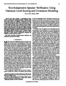
Figure 2.1: A block diagram of a text independent speaker verification system
2.2
Overview of speaker verification
The general process of speaker verification involves three stages: development, enrolment and verification, as is clearly shown in Figure 2.1. Development is the process of learning speaker independent parameters using the large amount of data that is to be used to learn about speech characteristics. Enrolment is the process of learning the distinct characteristics of a speaker’s voice and is used to create a claimed model to represent the enrolled speaker during verification. In verification, the distinct characteristics of a claimant’s voice are compared with the previously enrolled claimed speaker model to determine if the claimed identity is correct. Recent work in the field of speaker verification is mainly focused on the problem of the channel/ session variability between enrolment and verification segments, as it considerably affects the speaker verification performance. The channel/ session variability depends on the following factors,
16
2.3 Speech acquisition and front-end processing
Voice activity detection
Feature extraction
Feature domain channel compensation
Figure 2.2: A block diagram of a front-end processing • The microphones - carbon-button, electret, hands-free, array, etc • The acoustic environment - office, car, airport, etc. • The transmission channel - landline, cellular, VoIP, etc. • The differences in speaker voice - aging, mood, spoken language, etc.
Channel compensation is an approach which is used to reduce the mismatch between training and testing. Channel compensation occurs at the different levels, such as feature domain, model domain and score domain. In the feature domain, adaptive noise suppression, cepstral mean subtraction (CMS), RASTA filtering and feature warping are used to compensate the channel variability. JFA, JFASVM and i-vector approaches are used to compensate the mismatch between enrolment and verification in the model domain. In the score domain, score normalization approaches, such as test normalization (T-norm), symmetric normalization (S-norm) and zero test normalization (ZT-norm) are used to compensate the session variability. These approaches are briefly detailed in the following sections.
2.3
Speech acquisition and front-end processing
The front-end processing is used to process the audio and produce the features that are useful for speaker verification. The front-end processing generally con-
2.3 Speech acquisition and front-end processing
17
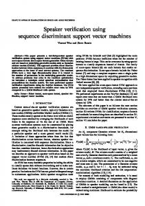
sists of three sub-processes as shown in Figure 2.2: VAD, feature extraction and feature-level channel compensation [5, 9, 83]. Firstly, the acquired speech is processed by a voice activity detection (VAD) system to ensure that the verification is only performed when speech is occurring. Gaussian-based VAD has been commonly used in recent times in which the distribution of both high energy and low energy frames are modelled. Frames belonging to the higher energy Gaussian are retained, and the remainder are removed from the feature set [81]. In this approach, VAD can operate successfully on audio with a relatively low signal-to-noise ratio (SNR) compared to other alternative approaches [63]. VAD is already in common use in telephony applications through standards, such as G729 Annex B [1, 4] or the ETSI Advanced Front-End [23]. The feature extraction approach is used to convert the raw speech signal into a sequence of acoustic feature vectors, carrying characteristic information about the signal, which can identify the speaker [93]. There are a number of feature extraction techniques available, including mel frequency cepstral coefficients (MFCC), linear prediction cepstral coefficients (LPCC) and perceptual linear prediction cepstral coefficients (PLPC) [28, 82]. All these features are based on the spectral information derived from a short time windowed segment of speech, and they mainly differ by the detail in the power spectrum representation. The MFCC and linear frequency cepstral coefficient (LFCC) features are derived directly from the fast fourier transform (FFT) power spectrum, whereas the LPCC and PLPC use an all-pole model to represent the smooth spectrum. Researchers have also found that phase spectrum-based features, such as modified group delay function (GDF) and instantaneous frequency deviation (IFD) can be also used to extract complementary speaker information [76, 76, 111]. The most commonly chosen feature extraction technique for the state-of-theart speaker verification system is MFCC as this feature representation has been
18
2.4 GMM-based speaker verification
FFT
||
Cosine transform
||
Figure 2.3: A block diagram of extracting the MFCC features shown to provide better performance than other approaches [28, 82]. A basic block diagram for extracting MFCC is given in Figure 2.3. The MFCC features are calculated through pre-emphasis filtering, framing and windowing, triangular filtering and discrete cosine transform (DCT). Time derivatives of the MFCC coefficients are used as additional features, and are generally appended to each feature to capture the dynamic properties of the speech signal [82]. The final stage of the front-end processing is the feature-domain channel compensation approach which will be discussed in Section 2.7.1.
2.4
GMM-based speaker verification
2.4.1
Brief overview of Gaussian mixture modelling
Gaussian mixture models (GMMs) were proposed by Reynolds et al. [83, 86, 87] to model the speaker, and they perform very effectively in speaker verification systems. A GMM is a weighted sum of M component Gaussian densities as given by the equation, P (x | λ) =
M X k=1
wk × g(x | µk , Σk )
(2.1)
2.4 GMM-based speaker verification
19
where x is a D-dimensional feature vector, wk , µk , Σk , k = 1, 2, ...........M , are the mixture weights, mean and covariance. g(x | µk , Σk ), k = 1, 2, 3.........M , are the component Gaussian densities. Each component density is a D-variate Gaussian function of the form, � � 1 1 T −1 g(x | µk , Σk ) = − (x − µk ) Σk (x − µk ) 1 exp D 2 (2π) 2 |Σk | 2
(2.2)
where mean vector µk and covariance matrix Σk , the mixture weights satisfy P the constraint M k=1 wi = 1. The complete GMM is parameterized by the mean vectors, covariance matrices and mixture weights from all component densities, and these parameters are collectively represented by λ = {wk , µk , Σk }, k = 1, 2, 3.........M . An expectation-maximization (EM) algorithm is an iterative method for finding maximum likelihood or maximum a posteriori estimates of parameters in statistical models. The EM algorithm is used to learn the GMM parameters, based on maximizing the expected log-likelihood of the training data. The motivation of the EM algorithm is to estimate a new and improved model λ from the current model λold using the training utterance features xn such that the probaQ QN old bility N n=1 P (xn | λ) ≥ n=1 P (xn | λ ). This is an iterative technique where the new model becomes the current model for the following iteration. The initial GMM parameters are typically defined using the k-means algorithm often used in the vector quantisation approach [33]. The k-means algorithm is also based on an iterative approach in which the mixture of training feature vectors is performed through the estimation of mixture means. The EM algorithm attempts to maximise the auxiliary function Q(λ; λold ). This Q is generally implemented using Jensen’s inequality ensuring N n=1 P (xn | λ) ≥
20 QN
n=1
2.4 GMM-based speaker verification P (xn | λold ). The auxiliary function can be formulated as old
Q(λ; λ ) =
N X M X
P (k | xn ) logwk g(xn | µk , Σk )
(2.3)
n=1 k=1
where P (k | x) forms the E step for producing observation x using P (k | x) =
wk g(x | µk , Σk ) P (x | λold )
(2.4)
The M step then sees the auxiliary function Q(λ; λold ) maximised using Equation 2.3. This maximisation results in the GMM parameters being estimated as N nk X wk = P (k | xn , λold ) T n=1
(2.5)
N 1 X µk = P (k | xn , λold )xn nk n=1
(2.6)
N 1 X P (k | xn , λold )xn xTn − µk µTk Σk = nk n=1
(2.7)
where nk is the component occupancy count from all the observations of the utterance x.
2.4.2
Universal background model (UBM) training
In typical speaker verification tasks, as there is a limited amount of data available to train the speaker models, the speaker models can’t be directly estimated reliably with the expectation maximization (EM) algorithm. For this reason, maximum a posteriori (MAP) adaptation [86] is often used to train the speaker models for speaker verification systems. This approach estimates the speaker model from the universal background model (UBM) [86]. A UBM is a high-order GMM, trained on a large quantity of speech obtained from a wide sample of the
2.4 GMM-based speaker verification
21
speaker population of interest, and is designed to capture the general form of a speaker model and represents the speaker-independent distribution of features. The UBM parameters are estimated using the EM algorithm described in the previous section.
2.4.3
Speaker enrolment through MAP adaptation
In MAP adaptation, the speaker model is derived from the UBM by considering specific speaker vectors. As a variant of the EM algorithm, first initializing the speaker models with the parameters of UBM iteratively updates the parameters of the GMM λ = {wk , µk , Σk } such that total likelihood for an enrolment utterance x1 , x2 ....xN is maximized: N Y
P (xn | λ) ≥
n=1
N Y
P (xn | λold )
(2.8)
n=1
The updated model is then used as the initial model for the next iteration. The process is repeated until some convergence threshold is reached. For each iteration of the EM algorithm, the expressions of the maximum likelihood (ML) estimates of the GMM parameters, which guarantee a monotonic increase of the model’s likelihood, are as described in the previous section. During the adaptation of the speaker models, common practice is to adapt only the means of the mixture components of the UBM to match the speaker characteristics, as it has been found that adapting the covariances do not show an improvement [86]. AP The MAP adapted means µM for Gaussian component k are updated from the k
prior distribution means µk using AP L µM = αk µk + (1 − αk )µM k k
(2.9)
22
2.4 GMM-based speaker verification
Development phase UBM Training Data
Enrollment Data
Front-end processing
GMM Training (m,Σ)
Front-end processing
MAP adaptation
∑UBM µ wUBM UBM
µ MAP Speaker Models Models Speaker
Enrollment phase Verification Data
Front-end processing
Verification phase
Likelihood test
D e c i s i o n
Figure 2.4: A block diagram of GMM-based speaker verification system L where µM is estimated using maximum likelihood estimation as detailed in prek
vious section and αk is the mean adaptation coefficient defined as αk =
nk nk +τk
where nk is the component occupancy count for the adaptation data and τk is the relevance factor, typically set between 8 and 32.
2.4.4
GMM-UBM speaker verification
The GMM-UBM-based speaker verification was the standard approach to textindependent speaker verification a decade ago [86]. Even though the data requirements with the MAP adaptation of UBM to obtain the speaker models in this approach are significantly less than the data requirements for estimating the speaker model directly, the technique sill requires a considerable amount of training data in order to take full advantage of the technique [86]. This is due to the large number of parameters that need to be estimated in the relevance MAP adaptation process of this technique. When limited training data is available, the model is unable to saturate, and the ability of the speaker model produced by
2.4 GMM-based speaker verification
23
the process to accurately represent the speaker is limited. A block diagram of a GMM-based speaker verification system is shown in Figure 2.4. In the development phase, the UBM parameters are estimated on a larger amount of data, which represents the speaker independent parameters. The MAP adaptation is used to estimate the speaker dependent parameters in the enrolment phase. In the verification phase, the scoring is calculated using the likelihood ratio. The task in speaker verification is to ascertain whether or not a test set of speech frames X = x1 , x2 , ..., xN belongs to the claimed speaker s. With generative models, the aim is to test the following hypotheses:
• Htar : X is uttered by speaker s • Himpo : X is not uttered by speaker s
The decision score is based on a likelihood ratio. It is evaluated by the following formula: S(X) =
P (X | Htar ) ≥ Θ ⇒ target P (X | Himpo )
(2.10)
where P (X | Htar ) and P (X | Himpo ) are respectively the likelihood of X under the assumption that X is uttered or not by speaker s, and Θ represents a decision threshold. If the computed score S(X) is greater than the decision threshold Θ, we conclude that test segment X is indeed uttered by speaker s. Otherwise, speaker s is deemed to be an impostor.
24
2.5 GMM super-vectors
Number of Gaussian components (1……..512)
µ1 µ 26
µ1 µ 26
µ1 µ1 ………... µ µ 26 26
MAP adapted individual Gaussian mean
=
µ1 µ 26 µ1 µ 26 µ1 µ 26 13312×1 GMM supervector
Figure 2.5: A block diagram of extracting GMM super-vectors
2.5
GMM super-vectors
In the GMM-UBM speaker verification system, MFCC acoustic features are used as input features. On the other hand, in SVM and JFA speaker verification systems, high-dimensional GMM super-vectors are used as input features. A block diagram of extracting GMM super-vectors is shown in Figure 2.5. The GMM mean super-vector is the concatenation of GMM mean vectors. It is defined by a column vector of dimension CF containing the means of each mixture component in the speaker GMM where F represents the dimensionality of the feature vectors used in the model and C denotes the total number of mixture components used to represent the GMM.
2.6
SVM-based speaker verification
SVMs have proven to be a new effective method for speaker verification [11, 13, 17, 74, 110]. SVM-based classifiers can be used to find a separator between two classes. SVM is a linear classification technique, and for the speaker verification task, a non-linear kernel mapping is generally required to project the non-linearly
2.6 SVM-based speaker verification
25
Development phase UBM Training Data
Enrollment Data
Feature Extraction
Feature Extraction
GMM Training (m,Σ)
∑UBM
µMAP
MAP adaptation
Background dataset
∑UBM
µUBM
SVM training
GMM supervector
Speaker SVM
Enrollment phase Verification Data
Feature Extraction
µMAP
SVM testing
GMM supervector
MAP adaptation
Verification phase
D e c i s i o n
Figure 2.6: SVM-based speaker verification system separable data into a high dimensional linearly separable space. A block diagram of an SVM-based speaker verification system is shown in Figure 2.6.
2.6.1
SVM classification
In speaker verification, one class consists of the target speaker training vectors (labelled as +1), and the other class consists of the training vectors from an impostor (background) population (labelled as -1). Using the labelled training vectors, SVM training finds a separating hyper plane that maximizes the margin of separation between these two classes. Formally, the discriminate function of SVM is given by, f (x) =
N X
αi ti K (x, xi ) + d
(2.11)
i=1
where ti ∈ {−1 + 1} are ideal output values,
PN
i=1
αi ti = 0 and αi ≥ 0
The support vectors xi , their corresponding weights αi and the bias term d, are
26
2.6 SVM-based speaker verification
Figure 2.7: An example of a two-dimensional SVM trained using (a) linearlyseparable data and (b) non-linearly-separable data (From [70]) determined from a training set using an optimization process.
2.6.2 Consider
Linearly separable training the
problem
of
separating
the
set
of
N
training
vectors
[(x1 , y2 ), ..., (xn , yn )] belonging to two different classes yi ∈ (−1, 1). The goal is to find the linear decision function D(x) and the separation plane H. An example of a two-dimensional SVM trained using linearly-separable data is given in Figure 2.7 (a). H :< w, x > +b = 0 D(x) = sign(w ∗ x + b)
(2.12) (2.13)
where b is the distance of the hyperplane from the origin and w is the normal to the decision region. Let the “margin” of the SVM be defined as the distance from the separating hyperplane to the closest two classes. The SVM training paradigm finds the separating hyperplane, which gives the maximum margin. The margin is equal
2.6 SVM-based speaker verification to
2 kwk
27
. Once the hyperplane is obtained, all the training examples satisfy the
following inequalities, xi ∗ w + b ≥ +1 for yi = +1
(2.14)
xi ∗ w + b ≥ −1 for yi = −1
(2.15)
We can summarize the above procedure to the following: Minimize 1 L(w) = kwk2 2
(2.16)
yi (xi ∗ w + b) ≥ +1, i = 1, 2, 3, 4, ......N
(2.17)
subject to
2.6.3
Non-linearly separable training
In the case of performing SVM training on non-linearly separable data, such as the 2-D example shown in Figure 2.7 (b), the miss-classification of training examples will cause the Lagrangian multipliers to grow exceedingly large and prevent a feasible solution. To account for such issues, a slack variable with an associated cost C must be introduced to penalize the miss-classification of training examples. This approach translates into a further constraint being placed on the Lagrangian multipliers, which is a strategy for finding the local maxima and minima of a function, such that 0 ≤ αi ≤ C
(2.18)
This approach can be viewed as introducing an additional soft margin extending from the hyperplane margin that only comes into effect when mis-classified
28
2.7 Combating training and testing mismatch
training examples are encountered. The larger the value of C, the more impact mis-classified training examples have on the location of the hyperplane.
Non-linear kernels: The application of kernel function to classical SVM classifiers allows more complex problems to be solved [16]. An SVM kernel is used to transform training and testing data into a higher dimensional space, which provides better linear separation. In non-linear classification, a kernel approach is done by defining the kernel function as, K(xi , xj ) = φ(xi ) ∗ φ(xj )
(2.19)
where φ(x) is a mapping function used to convert input vectors x to a desired space. The mapping function is selected on an application-specific basis as it defines the discriminative space in which linear classification is to be performed. There are a number of kernels that have been shown to work well for speaker classification. Those are GLDS kernel [10], the GMM mean super-vector kernel [13], MLLR kernel [96], frame-based kernel [109], sequence kernel [39], fisherkernel [109] and cosine kernel [20].
2.7
Combating training and testing mismatch
Feature-domain channel compensation approaches, model-domain channel compensation approaches, such as JFA and JFA-SVM, and score-domain approaches, including zero normalization (z-norm), test normalization (t-norm), symmetric normalization (s-norm) and zero test normalization (zt-norm), are discussed in this section.
2.7 Combating training and testing mismatch
2.7.1
29
Feature-domain approaches
Under the train-and-test mismatch condition, speech can be corrupted by channel, noise and transducer effects. In the feature-domain, channel compensation techniques, such as adaptive noise filtering, cepstral mean subtraction (CMS), RASTA filtering and feature warping, are used to compensate the effect of channel and slowly varying additive noise [24, 36, 77, 112]. In the signal domain, adaptive noise filtering is used to remove the wide band noise from speech signals [38, 112]. The basic idea of an adaptive noise cancellation algorithm is to pass the corrupted signal through a filter that tends to suppress the noise, while leaving the signal unchanged. This is an adaptive process which means it does not require a priori knowledge of signal or noise characteristics. A common method of improving the robustness of a feature set is CMS [24, 84]. This process reduces the effects of channel distortion by removing the mean from cepstral coefficients. It was also found that it removes the speaker-specific information with channel information, and subsequently, the cepstral mean and variance normalization (CMVN) was proposed as an extensive approach to CMS [102]. An alternate method to CMS and CMVN, the RASTA was proposed by Hermansky and Morgan [36] with the purpose of suppressing very slowly or very quickly varying components in the filter banks during the feature extraction. The RASTA filtering is essentially a band-pass filter used on the time trajectories of feature vectors extracted from speech. It has also been found that the RASTA also removes the speaker specific information in the low frequency bands. A few years ago, Pelecanos et al. [77] introduced the feature warping approach to speaker verification to compensate the effect of channel and slowly varying
30
2.7 Combating training and testing mismatch
additive noise in the feature domain. The authors found that the feature warping is a much more effective method to significantly compensate the non-linear distortions. The feature warping algorithm maps the distribution of cepstral feature vectors to a target distribution. As the target distribution is unknown, an assumption is made that the target distribution is a standard normal distribution. Feature warping provides a robustness to additive noise and linear channel mismatch while retaining the speaker specific information that can be lost when using CMS, CMVN and RASTA processing.
2.7.2
Model-domain approach (JFA)
A significant contributor to the performance degradation of traditional GMMUBM speaker verification is the presence of session variability between the training and testing conditions. The JFA approach has been introduced to combat the mismatch between training and testing [50, 53, 55, 56, 57, 58, 103]. The technique outlined below is based on the decomposition of the GMM mean super-vectors into speaker-dependent and session-dependent parts. Figure 2.8 illustrates that the JFA approach considers the variability of the GMM as a linear combination of the variability of the speaker and channel unobservable components: M=s+c
(2.20)
where s is the speaker super-vector and c is the channel (session) super-vector. The GMM super-vector M of a given utterance is therefore expressed as the sum of a speaker-dependent contribution s and a speaker independent session contribution c. The motivation behind the factor analysis is to explicitly model each of these contributions in a low-dimensional subspace of the GMM mean super-vector space in order to form a more accurate speaker GMM for speaker verification purposes.
2.7 Combating training and testing mismatch
Speaker space
31
M
S
C Channel space
Figure 2.8: M can be written as sum of speaker factors (s) and channel factors(c) We define s and c as s = m + Vy + Dz ch = Uxh
(2.21) (2.22)
where speaker dependant variable, y, and residual variable, z, are assumed to be independent and to have standard normal distributions; s is assumed to be normally distributed with mean m and covariance matrix vv∗ + d2 . In the above equations, the variable can be divided into the system hyper parameters (m, V, D, U) and the hidden speaker and session variables (x, y, z). These parameters are estimated using maximum likelihood and minimum divergence algorithms [50], where m - Speaker and session independent mean super vector- (CF × 1) U - Eigenchannel matrix (low dimension rectangular matrix - CF × Rc) V - Eigenvoice matrix (low dimensional rectangular matrix- CF × Rs) D - Residual scaling matrix(diagonal matrix - CF × CF )
32
2.7 Combating training and testing mismatch
xh - Session dependent variable y - Speaker dependent variable z - Residual variable There have been several approaches to the problem of estimating the hyper parameters which define the inter-speaker variability and inter-session variability model of the joint factor analysis [58]. Those are the classical MAP approach, eigenvoice MAP approach, eigenchannel MAP approach, joint estimation and decoupled estimation. The eigenvoice MAP and classical MAP are used to model the inter speaker variability. The eigenchannel MAP is used to model the intersession variability. The intersession variability in the spectral speech features is generally caused by channel transmission effects. It has also been found that the decoupled estimation gave the best performance compared with other estimation methods [56].
Classical MAP adaptation: Kenny et al. [56] proposed ML-based estimation of the a priori variance of the speaker population within a training corpus. In this new modelling, the super-vector s of a randomly chosen speaker can be written in the form of hidden variables as follows, s = m + Dz
(2.23)
where s is assumed to be normally distributed with mean m and covariance matrix d2 . MAP adaptation using a priori distribution is equivalent to ML training of the speakers when sufficient speaker data are available for adaptation. D is constraint to satisfy I = τ DT Σ−1 D. Here τ is relevance factor and Σ is diagonal matrix. If the number of mixture components C is large, classical MAP tends to saturate
2.7 Combating training and testing mismatch
33
slowly in the sense that large amounts of enrolment data are needed to use it to full advantage.
Eigenvoice MAP adaptation: Eigenvoice adaptation operates on the assumption of a low rank rectangular matrix V of dimension CF × Rs, with Rs � CF , that defines a representation of the speaker space [52]. The supervector s of a randomly chosen speaker is obtained by: s = m + Vy
(2.24)
where s is assumed to be normally distributed with mean m and covariance 0
matrix VV . When few observations are available, eigenvoice adaptation is more powerful than MAP adaptation for estimating speaker GMMs. Since we only need to estimate low dimensional hidden variable y. Eigenvoice adaptation is based on the assumption that the rank Rs of estimated matrix V is less than or equal to the number of speakers in the training corpus.
Combining relevance MAP and eigenvoice MAP: The strengths and weaknesses of classical MAP and eigenvoice MAP complement each other. If small amounts of data are available, eigenvoice MAP is preferable for speaker adaptation and if large amounts are available, classical MAP is preferable. Therefore, it is useful to assume that the speaker model takes a form which combines both relevance MAP and speaker subspace adaptation. The super-vector s of a randomly chosen speaker is obtained by, s = m + Vy + Dz
(2.25)
The two hidden vectors y and z are mutually independent and each vector has a standard normal prior distribution. The super-vector s follows a prior normal
34
2.7 Combating training and testing mismatch 0
distribution characterized by mean m and covariance matrix d2 + VV . We refer to the components of y as speaker factors and to the components of z as common factors.
Channel variability modelling: It is assumed in this formulation of the speaker model that the most significant session variability effects may also be described in a low-dimensional subspace of the full mean super-vector space. This allows for a channel compensation super-vector to be introduced into the speaker model, in order to minimize the effect of this inter-session variability. To achieve this, a speaker GMM may be considered as the combination of a session-independent speaker model with an additional offset of the model means representing the recording conditions of the session h. This can be expressed as ch = Uxh
(2.26)
where U - Eigenchannel matrix (low dimension rectangular matrix - CF × Rc) xh - session dependent variable This technique is referred to as eigenchannel adaptation, which has the same form as the eigenvoice adaptation procedure outlined in above section.
Mathematical representation of JFA modelling: First, a UBM is trained using the EM algorithm. The UBM is composed of C Gaussian components trained on F dimensional feature frames, and it can be characterized by weights w, a mean vector m (CF × 1) and covariance matrix Σ (CF × CF ). ˜ c (s) and The UBM is then used to extract the zero order, Nc (s), first order, F ˜ c (s), Baum-Welch statistics. Baum-Welch statistics are sufficient second order, S
2.7 Combating training and testing mismatch
35
statistics, which can be calculated using the following equations, Nc (s) =
X
˜ c (s) = F
X
γ t (c),
(2.27)
γ t (c)(Yt − mc ),
(2.28)
t
t
˜ c (s) = diag[ S
X
0
γ t (c)(Yt − mc )(Yt − mc ) ].
(2.29)
t
where c is the Gaussian index, γ t (c) is the posterior probability. Yt are MFCC feature frames and mc is UBM mean. The hyperparameter is calculated using the EM algorithm. The EM algorithm is performed in two steps. In the E step, we evaluate the posterior distribution of the hidden variable, y(s), given the speaker sufficient statistics and current hyperparameter, v estimation. Posterior distribution is calculated using BaumWelch statistics. Hidden variable, y(s) is calculated using following equations, l(s) = I + vT Σ−1 N(s)v, ˜ E[y(s)] = l−1 (s)vΣ−1 F(s), E[y(s)y(s)T ] = l−1 .
(2.30) (2.31) (2.32)
In the EM algorithm, the M step consists in updating the JFA hyperparameter, v, based on the expectations, E[y(s)] and covariance matrices, E[y(s)y(s)T ] of the hidden variable obtained in the previous step. We evaluate the hyperparameter, v using the following equations,
36
2.7 Combating training and testing mismatch
Maximum likelihood re-estimation, X Nc = Nc (s),
(2.33)
s
=c =
X
Nc (s)E[y(s)y(s)T ],
(2.34)
T ˜ F(s)E[y(s) ],
(2.35)
N(s).
(2.36)
s
∂=
X
N=
X
s
s
v, Σ is updated by solving the following equations, vi =c = ∂ i , Σ = N−1 [S(s) − diag(∂vT )].
(2.37) (2.38)
In the above calculations, pooling the Baum-Welch statistics is motivated by the fact that averaging the statistics over all utterances of each speaker removes the channel effects. All the JFA hyper-parameters are estimated iteratively in order to maximize the likelihood of the training corpus. The training database is composed of many speakers, and every speaker has several recordings under different channel conditions. The eigenchannel MAP model parameters can be calculated using a similar method of the above-mentioned eigenvoice MAP modelling.
JFA scoring: In the JFA approach, the calculated mean super-vector M is used to represent the speaker specific GMM in comparison to the background UBM, in order to provide more robustness to the session and intra-speaker variability than the traditional MAP approach. However, due to the unknown channel factor vector x, the JFA-calculated mean super-vector cannot be used directly as the speaker specific GMM super-vector in
2.7 Combating training and testing mismatch
37
ELLR score calculation. A number of approaches have been proposed to account for the channel factor:
• Integration over prior distribution • Channel point estimation • Linear approximation of channel point estimate
Glembek et al. [30] investigated different scoring techniques. While, in most cases, the performance of session variability does not change dramatically, the speed of evaluation is the major difference. The fastest scoring method is linear scoring. It can be implemented by a simple dot product, allowing for much faster scoring with little-to-no degradation in performance [30]. A block diagram of JFA-based speaker verification system is shown in Figure 2.9. In the development phase, the UBM parameters are learnt using the large amount of data to represent the speaker independent parameters, and the JFA hypoparameters (V, D, U) are estimated using maximum likelihood and minimum divergence algorithms. In the enrolment phase, the speaker variability hidden variables (y and z) are estimated for each target speakers. The channel variability hidden variable (x) for test speakers and scoring are calculated in the verification phase.
2.7.3
Model-domain approach (JFA-SVM)
Dehak et al. [21] investigated several techniques to combine the SVM and JFA model for speaker verification. In this combination, the SVMs are applied to different sources of information, such as GMM super-vectors, speakers and common factors which are produced by the JFA. It has been found that when the
38
2.8 Score normalization approaches
UBM Training Data
Feature Extraction
GMM Training (m,Σ)
JFA Training Data
Feature Extraction
BW Stats
JFA modeling
Feature Extraction
BW Stats
JFA Training Y, z
Enrollment Data
Development phase
m, sigma, V, D, U
JFA models
m+Vy+Dz
Speaker models
Enrollment phase Verification Data
Feature Extraction
BW Stats
JFA Training x
JFA Scoring
Verification phase
D e c i s i o n
Figure 2.9: A block diagram of JFA-based speaker verification system linear or cosine kernels are defined in speaker and common factors, the JFA-SVM achieves better performance than using the linear Kullback Leibler kernel [11, 21]. It has also been found that if the within-class covariance normalization (WCCN) approach, which is commonly used to attenuate the intra-speaker variance, is applied to speaker space to compensate the channel variation, JFA-SVM shows further improvement [21, 35]. In addition, the results of the JFA-SVM using the speaker factors are comparable to the classical JFA scoring [21].
2.8
Score normalization approaches
The decision-making process in speaker verification based on GMM-UBM is to compare the likelihood ratio obtained from the claimed speaker model and the UBM model with a decision threshold as previously shown in Section 2.4.4 [5]. Due to the score variability between the verification trials, the tuning of decision
2.8 Score normalization approaches
39
thresholds is an important and troublesome problem. Score variability mainly consists of two different sources. The first one is the different quality of speaker modelling caused by enrolment data varying. The second one is the possible mismatches and environment changes among test utterances when compared to the enrolment utterances. Score normalization means normalizing the distribution of the scores. There are four types of normalization methods [2]. Those are,
• Zero normalization (Z-norm) • Test normalization (T-norm) • Symmetric normalization (S-norm) • Combined normalization (ZT-Norm)
Z-norm: The z-norm addresses the problem of speaker score variability. It allows finding a decision threshold that is independent of the target speaker. For the z-norm, we consider J impostor segments X1 , X2 , ..., Xj . For each proclaimed identity L, we compute a speaker-dependent µL and σ L as follows: J
1X µL = S(Xj , λL ), J j=1 v u J u 1X t σL = [ (S(Xj , λL ) − µL )2 ]. J j=1
(2.39)
(2.40)
where S(Xj , λL ) is raw score of Xj impostor segment and L proclaimed identity. Z-norm can be calculated as follows, S(X, λL )norm =
S(X, λL ) − µL σL
(2.41)
40
2.8 Score normalization approaches
T-norm: The t-norm addresses the problem of session variability. It compensates the differences between the training and testing conditions. For the t-norm, we consider a set of impostor models λ1 , λ2 , .........λN . For each test segment X, we compute a test-dependent µX and σ X as follows: N
1 X µX = S(X, λn ) N n=1 v u N u 1 X t (S(X, λn ) − µX )2 ] σX = [ N n=1
(2.42)
(2.43)
T-norm can be calculated as follows, S(X, λL )norm =
S(X, λL ) − µX σX
(2.44)
S-norm: Symmetric normalization can be calculated using t-norm and z-norm scores as follows, S(X, λL )norm =
S(X, λL ) − µL S(X, λL ) − µX + σL σX
(2.45)
Combined normalization (ZT-norm): State-of-the-art systems often combine several score normalization techniques in order to boost performance. The application of Z-Norm followed by T-Norm (commonly called ZT-Norm) has been found to provide a dramatic improvement in speaker verification performance [7, 103]. By combining both normalization methods, both the speakercentric and test-centric advantages of the two individual techniques are combined.
2.9 Review of short utterance speaker verification
2.9
41
Review of short utterance speaker verification
For the wide deployment of speaker verification technology in practical applications, training and testing utterance length must be reduced below that required in current systems for user’s convenience. Li et al. [66] proposed an approach for the short utterances-based speaker verification system, which uses a statistical model of the speaker’s vector quantized speech. This technique retains textindependent properties while allowing considerably shorter test utterances than comparable speaker recognition systems. The speaker recognition performance depends on the statistical distribution of the distances between the speech frames from the unknown speaker and the closest points in the model, models were generated with 100 seconds of conversational training speech for each of 11 male speakers. The system was able to identify 11 speakers with 96%, 87%, and 79% accuracy from sections of unknown speech of durations of 10, 6, and 3 seconds, respectively. Jayanna et al. [40] investigated the multiple frame size and rate analysis for speaker recognition under limited data condition.
In typical state-of-the-art
speaker verification systems, fixed frame size and rate is used for feature extraction, which may be termed as single frame size and rate (SFSR) analysis. In a limited data condition, if the SFSR analysis is used, then it may not provide sufficient feature vector to train and test the speaker. In addition, an insufficient feature vector could lead to poor speaker modelling during training and may not yield a reliable decision during testing. The multiple frame size and rate techniques are specifically useful to mitigate the sparseness of limited feature vectors during training and testing. These techniques could produce relatively more numbers of feature vectors, and lead to better modelling and testing under limited
42
2.9 Review of short utterance speaker verification
data conditions. Thilo et al. [95] investigated a dimension-decoupled GMM-based speaker verification system with short utterances. A great challenge is to use these techniques in a situation where only small sets of training and evaluation data are available, which typically results in poor statistical estimates. Based on the observation of marginal MFCC probability densities, he has suggested to greatly reduce the number of free parameters in the GMM by modelling the single dimensions separately after proper pre-processing. Saving about 90% of the free parameters as compared to an already optimized GMM and thus making the estimates more stable, this approach considerably improves recognition accuracy over the baseline as the utterances get shorter and save a huge amount of computing time both in training and evaluation, enabling real-time performance. Vogt et al. [104, 106] investigated and compared the several alternative procedures for the factor analysis subspace estimation for speaker verification with short utterances, specifically focused on training and testing with short utterances. It was found that better performance can be obtained when independent rather than simultaneous optimization of the two core variability subspaces is used. Disjoint and coupled estimation of U and V have led to best performance. It was found that for verification trials on short utterances, it is important for the session subspace to be trained with matched length utterances [104]. It was also found that the factor analysis modelling approach to GMM speaker verification is an ideal solution for combining the benefits of speaker subspace MAP adaptation for short utterances and standard relevance MAP adaptation for longer utterances to provide a speaker modelling approach that is optimal over a wide range of utterance lengths [106]. McLaren et al. [73] investigated the effects of limited speech data in the context of speaker verification using the GMM mean super-vector SVM classifier.
2.10 Chapter summary
43
Verification performance was analysed with regards to the duration of impostor utterances used for background, score normalization and session compensation training cohorts. It was found that the duration of utterances used to train the background dataset have a considerable effect on classification performance. Matching these impostor utterances to test utterance length expected in trials was found to significantly improve SVM-based performance, and the NAP approach was seen to session compensation often degrade performance [73]. Vogt et al. [107, 108] proposed an approach to minimize the utterance length through the confidence-based early verification decisions. The early verification decision method, based on these confidence interval estimates, achieves a drastic reduction in the typical data requirements for producing confident decisions in an automatic speaker verification system. An average of 5-10 seconds of speech is sufficient to produce verification rates approaching those achieved previously, using an average in excess of 100 seconds of speech. A speech sample is gathered from a speaker over a period of time, and a verification score is then produced for said sample over period. Once the verification score is determined a confidence measure is produced based on frame score observations from said sample over the period and a confidence measure is calculated based on the standard Gaussian distribution.
2.10
Chapter summary
This chapter has detailed the overview of speaker verification technology, and has also explained the GMM- and SVM-based speaker verification systems. As mismatch between training and testing utterances considerably affects the speaker verification, several channel compensation approaches were introduced in difference levels to compensate the channel variations; these have been thoroughly
44
2.10 Chapter summary
explained in this chapter. In a typical speaker verification system, a significant amount of speech is required for model training and testing; however, it is hard to collect this amount of data in practical environments. A number of research studies have been conducted to solve this issue; they have been also detailed in this chapter.
Chapter 3 Speaker Verification using I-vector Features
3.1
Introduction
The previous chapter focused on GMM-based generative approaches and SVMbased discriminative approaches. Subsequently, GMM-UBM generative model approaches were also extended to the JFA approach to compensate the session variability, by modelling the speaker and channel variability separately [50]. Recent research in speaker verification has focused on the i-vector front-end factor analysis technique. This technique was firstly proposed by Dehak et al. [19, 20] to provide an intermediate speaker representation between the high dimensional GMM super-vector and traditional low dimensional MFCC feature representations. The extraction of these intermediate-sized vectors, or i-vectors, were motivated by the existing super-vector based JFA approach. The JFA approach models the speaker and channel variability space separately, whereas the i-vectors are formed by modelling a single low-dimensional total-variability space that covers
46
3.2 I-vector feature extraction
both speaker and channel variability [19, 20]. It is also believed that some of the speaker discriminant information may be lost in channel space in the JFA approach [20]. As the i-vectors are based on one variability space that contains speaker and channel variability information, compensation techniques are required to limit the effects of channel variability in the i-vector speaker representations. The channel compensation approaches play a major role in the i-vector speaker verification systems. When the i-vector approach was introduced, the several channel compensation approaches, including WCCN, linear discriminant analysis (LDA), nuisance attribute projection (NAP) and scatter difference NAP (SD-NAP) were used to compensate the channel variation in the i-vector speaker verification system [20]. Subsequently, Kenny noticed that each utterance can be represented by low-dimensional i-vector features, and introduced the PLDA to model the channel variability within the i-vector space [51]. This chapter is divided into several sub-parts. The i-vector feature extraction approach is detailed in Section 3.2. The cosine similarity scoring (CSS), or SVM ivector speaker verification system and standard channel compensation approaches are described in Section 3.3.1. The PLDA speaker verification system is described in Section 3.4.
3.2
I-vector feature extraction
In contrast to the separate speaker and channel dependent subspaces of the JFA, i-vectors represent the GMM super-vector using a single total-variability subspace. This single-subspace approach was motivated by the fact that the channel space of the JFA contains information that may be used to distinguish between
3.2 I-vector feature extraction
47
speakers [19, 20]. A speaker and channel dependent GMM super-vector, s, can be represented as follows; s = m + Tw,
(3.1)
where: m is the speaker and channel independent background UBM super-vector, T is the total-variability subspace which is a low rank matrix representing the primary directions’ variation across a large collection of development data. w is normally distributed with parameters N (0, 1), and is the i-vector representation used for speaker verification. The extraction of i-vectors is based on the BaumWelch zero-order, N, and centralized first-order, F, statistics. The statistics are calculated for a given utterance with respect to C UBM components and F dimension MFCC features. The i-vector for a given utterance can be extracted as follows [20], w = (I + TT Σ−1 NT)−1 TT Σ−1 F,
(3.2)
where I is a CF × CF identity matrix, N is a diagonal matrix with F × F blocks Nc I (c = 1, 2, ....C), and the super-vector, F, is formed through the concatenation of the centralized first-order statistics. The covariance matrix, Σ, represents the residual variability not captured by T. An efficient procedure of estimating the total-variability subspace, T, is described in [20, 58]. The process of training the total-variability space (T) is equivalent to JFA eigenvoice training except for one difference. In JFA eigenvoice training, all the sessions of given speaker are considered to be the same person but in total variability space training, all the sessions of given speaker are considered to be the different persons in order to capture the channel variation, as total-variability is used to capture both speaker and channel variations [20].
48
3.3
3.3 SVM/ CSS based i-vector speaker verification system
SVM/ CSS based i-vector speaker verification system
Inspired by the earlier use of JFA speaker factors directly as features for SVM classification, Dehak et al. [19] originally proposed an SVM/CSS i-vector speaker verification approach where i-vector features are directly used as features for SVM/CSS classifier. As i-vector features are based on one variability space, containing speaker and channel variability information, they have to combine with channel compensation approaches to remove the channel variability information. In SVM/CSS i-vector speaker verification system, channel compensation also occurs at several levels, such as feature domain, model domain and score domain. Feature warping techniques are commonly used in the feature domain, to provide a robustness to additive noise and linear channel mismatch while retaining the speaker specific information [77]. In the model domain, LDA followed by WCCN channel compensation approach is commonly used to compensate the channel variation [20]. In the score domain, t-normalization addresses the problem of session variability which compensates the mismatch between the enrolment and verification conditions [2]. As most channel variations occur at the model domain, the model domain channel compensation approaches are an active area of research, and several advanced channel compensation techniques will be introduced in the next chapter.
3.3.1
SVM and CSS classification techniques
Classification techniques, such as SVMs and CSS, are used with i-vector speaker verification systems [19, 20]. CSS is a computationally more efficient approach than SVMs, and it was also found that it provides better performance than SVM
3.3 SVM/ CSS based i-vector speaker verification system
49
approaches [20].
SVMs: SVM is used as a classifier to find the separation between two classes. SVMs’ kernel functions are used to project the input vectors into high dimensional feature space to obtain linear separability. These kernel functions allow us to compute the scalar product directly in the feature space, without defining the mapping function. Dehak et al. [19, 20] have found that the appropriate kernel ˆ test , and target i-vector, w ˆ target , is the cosine function between test i-vector, w kernel, calculated as, ˆ target , w ˆ test ) = K(w
ˆ target , w ˆ test i hw . ˆ target k kw ˆ test k kw
(3.3)
CSS: I-vectors were originally considered as a feature for SVM classification; however, fast scoring approaches using a cosine kernel directly as a classifier were found to provide better performance than SVMs with a considerable increase in efficiency [19]. The CSS operates by comparing the angles between a test i-vector, ˆ test , and a target i-vector w ˆ target : w ˆ target , w ˆ test ) = S(w
3.3.2
ˆ target , w ˆ test i hw . ˆ target k kw ˆ test k kw
(3.4)
Standard channel compensation approaches
As i-vectors are defined by a single variability space, containing both speaker and channel information, there is a requirement that an additional channel compensation approach be taken before verification. Channel compensation approaches are estimated based on the within- and between-class scatter variances. Withinclass scatter (within-speaker variability) depends on microphones, acoustic environments, transmission channel and differences in speaker voice. On the other
50
3.3 SVM/ CSS based i-vector speaker verification system
hand, between-class scatter (between-speaker variability) depends on speaker’ characteristics. These channel compensation techniques are typically designed to maximize the effect of between-class variability and minimize the effects of within-class variability.
WCCN: Hatch et al. [35] introduced the WCCN approach to SVM-based speaker verification systems. Later, Dehak et al. [20] used WCCN as a channel compensation technique to scale a subspace in order to attenuate dimensions of high within-class variance. For use in i-vector-based speaker verification, a within-class covariance matrix, W, is calculated using S ns 1 XX ¯ s )(wsi − w ¯ s )T , W= (ws − w S s=1 i=1 i
(3.5)
¯ s , is defined by, where the mean i-vector for each speaker, w ¯s = w
ns 1 X ws ns i=1 i
(3.6)
where S is the total number of speakers and ns is number of utterances of speaker s. In evaluation, the inverse of W is used to normalize the direction of the projected i-vector components, which is equivalent to scaling the subspace by the matrix B1 , where B1 B1 T = W−1 . The WCCN channel compensated iˆ WCCN ) can be calculated as follows, vector (w ˆ WCCN = B1 T w w
(3.7)
LDA: Dehak et al. [20] had also used an LDA approach as a channel compensation technique. LDA seeks to reduce dimensionality while preserving as much of the speaker discriminatory information as possible. This attempts to find a reduced set of axes A that minimizes the within-class variability while maximizing the between-class variability through the eigenvalue decomposition of Sb v = λSw v.
(3.8)
3.3 SVM/ CSS based i-vector speaker verification system
51
where the between-class, Sb , and within-class scatter, Sw , can be calculated as follows, Sb = Sw =
S X
¯ s − w)( ¯ w ¯ s − w) ¯ T, ns (w
s=1 S X ns X
¯ s )T . ¯ s )(wsi − w (wsi − w
(3.9)
(3.10)
s=1 i=1
¯ is defined by where the mean i-vector for across-all-speakers, w, S ns 1 XX ¯ = w ws N s=1 i=1 i
(3.11)
where N is the total number of sessions. ˆ LDA ) can be calculated as follows, The LDA channel compensated i-vector (w ˆ LDA = AT w w
(3.12)
NAP: NAP is also used to combat the session variations [94]. NAP attempts to remove the unwanted within-class variations from the feature vector. NAP matrix can be calculated as follows, P = I − VV
0
J(v) = vT Sw v S ns 1X 1 X s Sw = (w − w¯s )(wsi − w¯s )0 S s=1 ns 1=1 i
(3.13) (3.14) (3.15)
where I is the identity matrix and V can be obtained by applying an eigen decomposition to the matrix(S w ). The NAP-only channel compensated i-vector is calculated as follows, ˆ NAP = PT w w
(3.16)
52
3.3 SVM/ CSS based i-vector speaker verification system
SD-NAP: The NAP is, in current form, removing between-class scatter information from the feature space; this information can be used to discriminate between speakers. Vogt et al. [105] proposed that the SD-NAP minimizes this information loss. The SD-NAP extends on the NAP approach by incorporating the between-class scatter matrix in the eigenvalue problem. The SD-NAP can be calculated as follows, J(v) = vT (Sw − mSb )v S X ¯ ¯ 0 Sb = (ws − w)(w s − w)
(3.17) (3.18)
s=1
where Sb is the between-class scatter variance and m controls the influence of the between-class scatter variance. The SD-NAP-only channel compensated i-vector is calculated as follows, ˆ SD-NAP = PT w w
SN-LDA: McLaren et al.
(3.19)
found that the between-class scatter calculated
using the standard LDA approach can be influenced by source variation under mismatched conditions where sources were defined as microphone and telephone recorded speech [71, 72]. This influence can be reduced by estimating the between-class scatter using source-normalized i-vectors and fixing the within-class scatter as the residual variations in the i-vector space [71]. The source-normalized between-class scatter, Ssrc b , can be composed of the source-dependent betweenclass scatter matrices for telephone and microphone-recorded speech, which can be calculated as follows, tel mic Ssrc b = Sb + Sb
(3.20)
3.3 SVM/ CSS based i-vector speaker verification system
53
where Stel b = Smic = b
Stel X s=1 S mic X
¯s − w ¯ tel )(w ¯s − w ¯ tel )T , ns (w
(3.21)
¯s − w ¯ mic )(w ¯s − w ¯ mic )T , ns (w
(3.22)
s=1
P tel tel ¯ tel ) is equal to n1tel ni=1 where the mean i-vector for telephone source (w wi , mean P nmic 1 mic ¯ mic ) is equal to nmic i-vector for microphone source (w i=1 wi . Rather than estimating the within-class scatter separately as in Equation 3.10, McLaren et al. [71, 72] calculated the within-class scatter matrix as the difference between a total variance matrix, St , and the source-normalized between-class scatter: Sw = St − Ssrc b ,
(3.23)
where St =
N X
¯ ¯ T. (wn − w)(w n − w)
(3.24)
n=1
This approach allows Sw to be more accurately estimated when a development dataset does not provide examples of each speech source from every speaker. Similarly to the LDA approach outlined previously, the SN-LDA channel compensated i-vector is calculated using Equation 3.12.
Sequential channel compensation: Previously, several individual channel compensation techniques were detailed. Individual LDA techniques are generally used to increase the inter-speaker variability while minimizing the intra-speaker variability, and the WCCN approach is used to reduce the channel effect by minimizing the intra-speaker variability. Dehak et al. [20] found that the sequential approach of first transforming the subspace using LDA, and then further transforming the new subspace with WCCN (or, alternatively WCCN of LDA, represented as WCCN[LDA]) extracts more speaker discriminant features than
54
3.3 SVM/ CSS based i-vector speaker verification system
individual LDA and WCCN approaches, but continued research has found that any type of LDA followed by WCCN is generally the best approach [47, 71]. In the first stage of the WCCN[LDA] approach, LDA attempts to find a reduced set of axes A that minimizes the within-class variability while maximizing the between-class variability. The estimation of LDA (A) was briefly described in Section 3.3.2. In the second stage, WCCN is used as a channel compensation technique to scale a subspace in order to attenuate dimensions of high within-class variance. The WCCN transformation matrix (B2 ) is trained using the LDA-projected ivectors from the first stage. The WCCN matrix (B2 ) is calculated using Cholesky decomposition of B2 B2 T = W−1 , where the within-class covariance matrix W is calculated using W=
S ns 1 XX ¯ s ))(AT (wsi − w ¯ s ))T (AT (wsi − w S s=1 i=1
(3.25)
where wsi is the i-vector representation of i session of speaker s, the mean i-vector P s s ¯ s ) is equals to n1s ni=1 for each speaker (w wi , S is the total number of speakers and ns is number of utterances of speaker s. The WCCN[LDA]-channel-compensated i-vector can be calculated as follows, ˆ W CCN [LDA] = BT2 AT w w
3.3.3
(3.26)
I-vector score normalization
In the score domain, score normalization approaches, t-, z- and zt-norm, are commonly used with i-vector speaker verification, and previous studies also found that zt-norm performs better than t- and z-norm approaches [20]. Dehak et al. [18] also introduced a modification to the CSS that does not require explicit score
3.4 PLDA speaker verification
55
normalization, relying on simple mean and covariance statistics from a collection of impostor speaker i-vectors. This new scoring simulates zt-norm, and can be calculated as follows, ˆ target , w ˆ test ) = S(w
ˆ target − w ˆ imp )(w ˆ test − w ˆ imp ) (w . ˆ target k kCimp .w ˆ test k kCimp .w
ˆ imp is the mean of imposter i-vectors. where w
(3.27)
Cimp is a diagonal matrix,
which contains the square root of the diagonal covariance matrix of the impostor i-vectors. In our experiments, zt-norm was used as there is no difference performance-wise, between this new scoring and the zt-norm.
3.4
PLDA speaker verification
The standard channel compensation approaches CSS/SVM i-vector speaker verification system was detailed in the previous section. Rather than attempting to compensate the channel variability in the i-vector space, recently, Kenny [51] has introduced the PLDA approach where the channel variability can be modelled within the i-vector space. As i-vector features are smaller in size, this allowed him to investigate the PLDA-based generative approach with speaker verification systems. The PLDA technique was originally proposed by Price et al. [80] for face recognition, and later it was adapted for modelling the i-vector distributions for speaker verification [8, 51, 88]. Two PLDA approaches, GPLDA and HTPLDA were introduced [51]. It was also found that the HTPLDA approach achieved a significant improvement over the GPLDA approach on the standard NIST SRE conditions as more closely modelled the true heavy-tailed distribution of i-vector features [51]. Recently, Garcia-Romero et al. [29] found that the heavy-tailed behaviour of i-vector features can be converted into Gaussian behaviour by using the length-normalized approach, and the length-normalized GPLDA has shown similar performance as the HTPLDA.
56
3.4 PLDA speaker verification
Previously Dehak et al. [20] proposed that FA be used as a feature extractor to extract low dimensional i-vectors (total variability factors). Subsequently, Kenny proposed that the i-vectors, wr , can be decomposed into speaker part, ¯s, and channel part, c¯r . wr = ¯s + c¯r
(3.28)
wr = m + U1 x1 + U2 x2r + εr
(3.29)
where for given speaker recordings r = 1, .....R; U1 is the eigenvoice matrix and U2 is the eigenchannel matrix, x1 and x2r are the speaker and channel factors respectively and εr is the residuals. In PLDA modelling, the speaker specific part is represented as U1 x1 . The covariance matrix of the speaker part is U1 U1 T , which represents the between-speaker variability. The channel specific part is represented as U2 x2r + εr . The covariance matrix of the channel part is Λ−1 + U2 U2 T , which describes the within-speaker variability, where Λ is the precision matrix of residual factors. It is assumed that speaker part (s) and channel part (c) are statistically independent [51]. Extra notation is introduced as follows, + + + wr = U + 1 x1 + U2 x2r + εr
(3.30)
where x+ 1 is the vector of dimension (N1 + 1) × 1 obtained by appending 1 to x1 + and similarly for x+ 2r . U1 is the matrix of dimension F × (N1 + 1) obtained by
appending a column vector m1 to U1 and similarly for U+ 2r , and m1 + m2 = m. The mathematical derivations in Sections 3.4.1 and 3.4.2 are based on work of Kenny [51].
3.4 PLDA speaker verification
3.4.1
57
GPLDA
For the Gaussian case, the speaker factor (x1 ) is assumed to be a vector having a standard normal distribution of dimension N1 , the channel factor (x2r ) is assumed to be a vector having a standard normal distribution of dimension N2 , and the residual (εr ) is an F -dimensional vector having a normal distribution with mean 0 and precision matrix (Λ). The graphical representation of GPLDA is shown in Figure 3.1 where the boxes denote plates. The R plate represents the R recordings of given speakers. The shaded circular node represents the observed variables, and the unshaded circular node indicates hidden variables [51].
Figure 3.1: Graphical representation of GPLDA model. From [51]
Mathematical representation of the GPLDA modelling: R recordings of single speaker are used to calculate the posterior distribution of the hidden variables. The posterior distribution ln P (x1 , x2r | wr ) is calculated using variational approximation form, ln P (x1 , x2r | wr ) ' ln Q(x1 ) +
R X r=1
ln Q(x2r )
(3.31)
58
3.4 PLDA speaker verification
where Q(x1 ) and Q(x2r ) are Gaussian distribution.
Updating the Gaussian distribution parameters: The mean and covariance of Q(x1 ) and Q(x2r ) are estimated by, Cov(x1 , x1 ) = (I + RUT1 ΛU1 )−1 , hx1 i = (I +
RUT1 ΛU1 )−1
×
(3.32) R X
+ UT1 Λ(wr − m1 − U+ 2 hx2r i),
(3.33)
r=1
Cov(x2r , x2r ) = (I + UT2r ΛU2r )−1 ,
(3.34)
+ hx2r i = (I + UT2r ΛU2r )−1 × UT2r Λ(wr − m2 − U+ 1 hx1 i).
(3.35)
Likelihood calculations: The likelihood of P (w | x) is estimated as follows, ln P (w | x) = K − 0.5(ln det(Λ) ∗ + T ∗ + ∗ + + (wr − U∗1 x+ 1 − U2r x2r ) Λ(wr − U1 x1 − U2r x2r ))
(3.36)
where K is a constant, and L1 = ln P (w | x)
Maximum likelihood estimation: Model parameters U1 , U2 and Λ are estimated using maximum likelihood estimation by maximizing L1 . It is equivalent to minimizing the following equation, R XX s
h(wr (s) − Wzr (s))T Λ(wr (s) − Wzr (s))i
r=1
+ where W = (U+ 1 U2 ).
W is calculated by estimating the derivative of the above equation, and that leads to the below formula, W
R XX s
r=1
hzr (s)zTr (s)i =
R XX s
r=1
wr (s)hzTr (s)i
(3.37)
3.4 PLDA speaker verification
59
where hzr i = hzr zTr i =
hx+ 1i
hx+ 2r i
(3.38)
+ T hx+ 1 (x1 ) i
+ T hx+ 1 (x2r ) i
+ T + + T hx+ 2r (x1 ) i hx2r (x2r ) i
(3.39)
where + T hx+ 1 (x1 ) i =
+ Cov(x1 , x1 ) + hx1 ihx+ 1 i hx1 i
hx1 i
1
(3.40)
+ T hx+ 2r (x2r ) i is evaluated similarly.
Λ is estimated by, Λ = ( R1
P PR s
r=1 h(wr (s)
− Wzr (s))(wr (s) − Wzr (s))T i)−1
(3.41)
Minimum divergence estimation: The minimum divergence algorithm is applied to modal parameters and hidden variables to speed up convergence. A minimum divergence estimate of eigenvoice parameters, (x1 (s), U1 , m1 ), are given by, 0
x1 (s) = A(x1 (s) − a), 0
U1 = U1 A−1 , 0
m1 = m1 + U1 a.
(3.42) (3.43) (3.44)
where a=
1X hx1 (s)i, S s
A−1 = L.
(3.45) (3.46)
60
3.4 PLDA speaker verification
and L is calculated from Cholesky decomposition of 1X hx1 (s)x1 (s)T i − aaT S s The
minimum
divergence
estimate
of
the
eigenchannel
parameters,
(x2r (s), U2r , m2 ), are given by, 0
x2r (s) = A(x2r (s) − a), 0
U2 = U2 A−1 , 0
m2 = m2 + U2 a.
(3.47) (3.48) (3.49)
where, R
a=
1 XX hx2r (s)i, R s r=1
A−1 = L.
(3.50) (3.51)
and L is calculated from Cholesky decomposition of R
1 XX hx2r (s)x2r (s)T i − aaT R s r=1 A major drawback of GPLDA approach is the lack of robustness to outliers in the speaker and channel subspaces [51]. In order to account with these outliers, Kenny [51] proposed that Student’s t-distribution can be used as an alternative to the Gaussian for modelling the subspaces.
3.4.2
HTPLDA
As Student’s t-distribution has heavy-tail behaviour compared to the exponentially-decaying tails of a Gaussian behaviour, this approach provides a better representation of outliers encountered in the i-vector space [61]. For the
3.4 PLDA speaker verification
61
Figure 3.2: Graphical representation of HPLDA model. From [51] heavy-tailed case, speaker factor(x1 ), channel factor(x2r ) and residual(εr ) have student’s t distribution. It is assumed that, x1 ∼ N (0, u1 −1 I) where u1 ∼ G(n1 /2, n1 /2)
(3.52)
x2r ∼ N (0, u2r −1 I) where u2r ∼ G(n2 /2, n2 /2)
(3.53)
εr ∼ N (0, vr −1 Λ−1 ) where vr ∼ G(v/2, v/2)
(3.54)
where n1 , n2 and v are the number of degree of freedom and u1 , u2r and vr are scalar-value hidden variables. The graphical representation of HPLDA is shown in Figure 3.2. The shaded small circles represent the model parameters.
Mathematical representation of HTPLDA modelling: R recordings of single speaker are used to calculate the posterior distribution of the hidden variables. The posterior distribution ln P (x, u, v | w) is estimated using the varia-
62
3.4 PLDA speaker verification
tional approximation form, ln P (x, u, v | w) ' ln Q(x1 ) +
R X
ln Q(x2r ) + ln Q(u1 ) +
r=1
+
R X
R X
ln Q(u2r )
r=1
ln Q(vr )
(3.55)
r=1
where Q(u1 ), Q(u2r ) and Q(vr ) are Gamma distribution, Q(x1 ) and Q(x2r ) are Gaussian distribution.
Updating Gaussian distribution parameters: The mean and covariance of Q(x1 ) and Q(x2r ) are estimated by, Cov(x1 , x1 ) = (hu1 iI + hx1 i = (hu1 iI +
R X r=1 R X
hvr iUT1 ΛU1 )−1 hvr iUT1 ΛU1 )−1
r=1
(3.56) ×
R X
hvr iUT1 Λ(wr − m − U+ 2 hx2r i)
r=1
(3.57) Cov(x2r , x2r ) = (hu2r iI + hvr iUT2r ΛU2r )−1
(3.58)
hx2r i = (hu2r iI + hvr iUT2r ΛU2r )−1 × hvr iUT2r Λ(wr − m − U+ 1 hxr i) (3.59) where the expectation, hu1 i, hu2r i and hvr i, are calculated from posteriors Q(u1 ), Q(u2r ) and Q(vr ).
Updating Gamma distribution parameters: The parameters of Q(u1 ) are given by, n1 + N1 2 n1 + hxT1 x1 i b1 = 2 a1 hu1 i = b1 a1 =
hln u1 i = ψ(a1 ) − ln(b1 )
(3.60) (3.61) (3.62) (3.63)
3.4 PLDA speaker verification
63
The parameters of Q(u2r ) are given by, n2 + N2 2 n2 + hxT2r x2r i b2r = 2 a2r hu2r i = b2r a2r =
hln u2r i = ψ(a2r ) − ln(b2r )
(3.64) (3.65) (3.66) (3.67)
The parameters of Q(vr ) are given by, ν+F 2 ν + h�Tr Λ�r i βr = 2 αr hvr i = βr αr =
hln vr i = ψ(αr ) − ln(βr )
(3.68) (3.69) (3.70) (3.71)
where h�Tr Λ�r i = tr(UT1 ΛU1 Cov(x1 , x1 ) + UT2 ΛU2 Cov(x2r , x2r )) + h�Tr iΛh�r i (3.72) + h�r i = wr − U+ 1 x1 − U2 x2r
(3.73)
Likelihood Calculations: The likelihood of P (w) is calculated by marginalizing P (w, h) with respect to hidden variables h (x, u, v). Lower bound L as a
64
3.4 PLDA speaker verification
proxy for ln P (w), and it is estimated as follows, Z P (w) = P (w, h)dh L = E[ln
(3.74)
P (w, h) ] Q(h)
(3.75)
L = L1 + L2
(3.76)
L1 = E[ln P (w | h)]
(3.77)
L2 = −D(Q(h) k P (h))
(3.78)
L1 =
R X 1 F 1 − ( hln vr i + ln hvr ih�Tr Λ�r i) 1 F −1 2 2 (2π) 2 (det(Λ )) 2 r=1
L2 = D(Q(x1 , u1 ) k P (x1 , u1 )) +
R X
(3.79)
D(Q(x2r , u2r ) k P (x2r , u2r ))
r=1
+
R X
D(Q(vr ) k P (vr ))
(3.80)
r=1
where D( k ) denotes the Kullback-Leibler divergence. D(Q(x1 , u1 ) k P (x1 , u1 )) = −
N1 N1 1 − hln u1 i − ln det(Cov(x1 , x1 )) 2 2 2
1 + hu1 ihxT1 x1 i + D(Q(u1 ) k P (u1 ) 2
(3.81)
Maximum likelihood estimation: Model parameters U1 , U2 and Λ are estimated using maximum likelihood algorithm by maximizing L1 , W
R XX s
hvr (s)ihzr (s)zTr (s)i
=
R XX
r=1
s
hvr (s)wr (s)hzTr (s)i
(3.82)
r=1
where hzr i = hzr zTr i =
hx+ 1i
hx+ 2r i
+ T hx+ 1 (x1 ) i
(3.83) + T hx+ 1 (x2r ) i
+ T + + T hx+ 2r (x1 ) i hx2r (x2r ) i
(3.84)
3.4 PLDA speaker verification
65
where
Cov(x1 , x1 ) +
+ T hx+ 1 (x1 ) i =
hx1 ihx+ 1i
hx+ 1i
hx1 i
1
(3.85)
+ T and hx+ 2r (x2r ) i is evaluated similarly.
Λ is estimated by, Λ = ( R1
P PR s
r=1 hvr (s)ih(wr (s)
− Wzr (s))(wr (s) − Wzr (s))T i)−1 (3.86)
Minimum divergence estimation: Minimum divergence algorithm is applied to modal parameters (U1 , U2 , m, p) and hidden variables (x1 , x2r , u1 , u2r , vr ), to speed up convergence.
A minimum divergence estimate of eigenvoice
(x1 (s), U1 , u1 , m1 , ) parameters is estimated by, 0
x1 (s) = A(x1 (s) − a), 0
U1 = U1 A−1 , 0
m1 = m1 + U1 a, 0
u1 (s) = ku1 (s).
(3.87) (3.88) (3.89) (3.90)
where S , s hu1 (s)i X 1 a= P hu1 (s)ihx1 (s)i, s hu1 (s)i s k=P
A−1 = L. L is calculated from Cholesky decomposition [60] of
P
X 1 hu1 (s)ihx1 (s)x1 (s)T i − aaT hu (s)i s 1 s
(3.91) (3.92) (3.93)
66
3.4 PLDA speaker verification
Minimum divergence estimate of eigenchannel (x2r (s), U2r , u2r , m2 ) parameters are given by, 0
x2r (s) = A(x2r (s) − a), 0
U2 = U2 A−1 ,
(3.94) (3.95)
0
m2 = m2 + U2 a, 0
u2r (s) = ku2r (s).
(3.96) (3.97)
where, k = P PR s
r=2 hu2r (s)i
a = P PR s
R
,
(3.98)
R XX
1
r=1 hu2r (s)i
s
hu2r (s)ihx2r (s)i,
(3.99)
r=1
A−1 = L.
(3.100)
L is calculated from Cholesky decomposition[60] of 1 P PR s
r=1 hu2r (s)i
R XX hu2r (s)ihx2r (s)x2r (s)T i − aaT s
r=1
Minimum divergence estimate of precision (vr (s), Λ) parameters are given by, 0
Λ =
Λ , k
0
vr (s) = kvr (s).
(3.101) (3.102)
where k is calculated as follows, R k = P PR
r=1 hvr (s)i
s
Degree of freedom (n1 , n2 , ν) are calculated using following equations, n1 1X n1 =1+ (hln u1 (s)i − hu1 (s)i), ψ( ) − ln 2 2 S s
(3.103)
(3.104)
R
ψ(
n2 n2 1 XX ) − ln =1+ (hln u2r (s)i − hu2r (s)i), 2 2 R s r=1
(3.105)
R
ν ν 1 XX ψ( ) − ln = 1 + (hln vr (s)i − hvr (s)i). 2 2 R s r=1 The above equations can be solved by newton raphson method.
(3.106)
3.4 PLDA speaker verification
3.4.3
67
Length-normalized GPLDA
Recently, Garcia-Romero et al. [29] have found the way to convert the i-vector feature behaviour from heavy-tailed to Gaussian. They have introduced the length-normalization approach, and it has shown a similar performance as HTPLDA and a more computationally efficient approach than HTPLDA. The lengthnormalization approach is used to transform the non-Gaussian i-vector feature behaviour into Gaussian i-vector feature behaviour [68]. This technique follows two steps: (1) linear whitening and (2) length-normalization. A linear whitened i-vector, wwht , can be estimated as follows, 1
wwht = d− 2 UT w
(3.107)
where Σ is a covariance matrix, which is estimated using development i-vectors. U is an orthonormal matrix containing the eigenvectors of Σ and d is a diagonal matrix containing the corresponding eigenvalues. Length-normalized i-vector feature, wnorm , can be calculated as follows, wnorm =
wwht kwwht k
(3.108)
If the i-vector feature behaviour is standard Gaussian distribution, the length distribution of i-vector features should follow a Chi distribution with number of degrees of freedom (DOF) equal to the dimension of the i-vector. GarciaRomero et al. [29] have found that the length distribution of development and evaluation data i-vectors fails to match the Chi distribution, and the mismatch led to a conclusion that i-vector feature is having heavy-tailed behaviour. The authors have also shown in [29] that length normalization approach can be used to transform the non-Gaussian i-vector feature behaviour into Gaussian i-vector feature behaviour. We illustrate this finding by Garcia-Romero et al et al., in Figure 3.3 by choosing
68
3.4 PLDA speaker verification
9
Original i-vector Length-normalized i-vector
8 7 6 5 4 3 2 1 0 −3
−1
−2
0
1
2
3
Figure 3.3: Histogram of original and length-normalized values of the nth i-vector feature, where n was randomly selected. an arbitrary speaker. A speaker (1148-sre04) and dimension (n) were randomly selected for a histogram plot to illustrate the effect of length-normalisation of i-vectors. It can be seen, by comparing the histograms of standard i-vectors and length-normalized i-vectors in the Figure 3.3, that i-vector feature behaviour is moving from Heavy-tailed to Gaussian.
3.4.4
PLDA scoring
GPLDA, HTPLDA and length-normalized GPLDA based i-vector system’s scoring is calculated using batch likelihood ratio [51]. Batch likelihood calculation is computationally more expensive than cosine distance scoring. Given two i-vectors wtarget and wtest , batch likelihood ratio can be calculated as follows, ln
P (wtarget , wtest | H1 ) P (wtarget | H0 )P (wtest | H0 )
(3.109)
where H1 : the speakers are same, H0 : the speaker are different. Lower bound L as a proxy for the log likelihood and it is estimated using Equation 3.77.
3.5 Chapter summary
69
P (wtarget , wtest | H1 ) is estimated using wtarget and wtest utterances by evaluating the L when R equals 2. P (wtarget | H0 ) and P (wtest | H1 ) are respectively estimated using wtarget and wtest utterances by evaluating the L when R equals 1.
3.5
Chapter summary
In recent times, CSS i-vector and PLDA speaker verification systems have become state-of-the-art approaches, and these two approaches deeply detailed in this chapter. Initially, this chapter detailed the i-vector feature extraction approach, standard channel compensation approaches, including LDA and WCCN, and cosine similarity scoring. Subsequently, GPLDA, HTPLDA, and length-normalized GPLDA approaches were also detailed. These two speaker verification systems will be used to evaluate the newly proposed techniques in next chapters.
Chapter 4 Speaker Verification Framework
4.1
Introduction
In recent times, CSS i-vector and PLDA speaker verification systems have become state-of-the-art techniques [20, 51]; these approaches were extensively detailed in the previous chapter. For the experimental work in this thesis, a comprehensive framework was required. The framework of CSS i-vector and PLDA speaker verification systems and experimental protocol, which is used to train the systems, are detailed in this chapter. It is also explained how short-length utterances are extracted from long-length utterances.
72
4.2
4.2 An overview of speaker verification databases
An
overview
of
speaker
verification
databases The switchboard series of corpora: The Switchboard series of corpora was collected by the Linguistic Data Consortium (LDC) [31]. Switchboard I consisted of landline-based telephony speech from both electret and carbon-button handset types. This corpus was collected from 543 U.S. participants with a total of 4800 conversation sides or speech segments. Switchboard II consisted of three separate phases differing in demographic region; Mid-Atlantic, Midwest, southern regions respectively. The majority of participants were sourced from local universities. Switchboard II Phase I consisted of 3638, 5-minute telephone conversations from 657 participants. Phase II consisted of 4,472 conversations involving 679 participants [31]. Phase III used 5,456 sides from 640 participants under varied environmental conditions. The Switchboard Cellular series of corpora was released in two parts in 2001 and 2004 respectively. Part 1 focussed primarily on GSM cellular phone technology with a total of 2618 sides (1,957 from GSM cell phones) from 254 participants roughly divided in gender. Part 2 focussed on cellular phone technology from a variety of service types, with CDMA technology being most dominant due to its popularity at the time of collection. A total of 4,040 sides (2,950 cellular) from 419 participants were recorded under a variety of environmental conditions [12].
NIST databases (years 2004 to 2006): In 2004, the NIST SRE presented a new evaluation protocol in which the previous core condition and extended evaluation tasks were combined [97]. In this way, evaluations could include training data from 10 seconds through to 16 training sides with test conditions using speech segments of 10 seconds to a full conversation side. All participating sites, however, were required to perform the compulsory one side train-one side test
4.2 An overview of speaker verification databases
73
condition of the evaluation with all other conditions being optional. The NIST 2006 SRE reused a proportion of the data from the 2005 SRE which, consequently, presented difficulties during the system development process due to the potential overlap in speakers between the development and unseen data. The difficulties associated with diverse and substantial data collection resulted in the following NIST SREs being held every two years [98].
NIST databases (years 2008 to 2010): The NIST 2008 SRE saw the introduction of several challenging tasks. Most dominant of these was the use of conversational speech data recorded using a microphone in an interview type scenario and taken from the Mixer 5 Interview speech corpus [99]. Additionally, conversational telephone speech was recorded over a microphone channel to introduce a new test condition. The use of interview style data allowed longer speech segments (approximately 15 minutes) to be used for training and testing. A proportion of target speakers from the NIST 2006 SRE were also present in the 2008 SRE, however, there was no overlap in speech segments between the corpora. The 2010 evaluation is similar to that of 2008 but different from prior evaluations by including in the training and test conditions for the core (required) test, not only conversational telephone speech recorded over ordinary (wired or wireless) telephone channels, but also such speech recorded over a room microphone channel, and conversational speech from an interview scenario recorded over a room microphone channel [100]. But unlike in 2008 and in prior evaluations, some of the data involving conversational telephone style speech have been collected in a manner to produce particularly high, or particularly low, vocal effort on the part of the speaker of interest. Unlike 2008, the core test interview segments are of varying duration, ranging from three-to-fifteen minutes.
74
4.3 Performance measures
The 2010 evaluation primarily uses recently collected speech data from speakers not included in previous evaluations, but also included some old and new conversational telephone speech segments from speakers in various past evaluations. Some new speech has recently been collected from speakers appearing in earlier evaluations.
4.3
Performance measures
Speaker verification performance is typically measured using the equal error rate (EER) and minimum decision cost function (DCF) [85]. These measures represent different performance characteristics of a system, however, their accurate estimation relies on a sufficient number of trials to be evaluated in order to robustly calculate the relevant statistics. System performance can also be represented graphically to assist in the direct comparison of systems. For such a task, the detection error trade-off (DET) plots are utilised. The performance of a speaker verification system can be represented by two specific types of errors; false alarms (false acceptance), and missed detections (false rejection). A false alarm occurs when a speech segment from an impostor speaker is incorrectly identified as originating from the target speaker. On the other hand, a missed detection (false rejection) refers to the rejection of the target speaker from the system. There exists a trade-off between these two types of error such that a system can be tuned to a specific application-dependent operating point. With regard to performance metrics, the EER provides a measure of missed detections and false alarms when defining the decision threshold to cause an equal proportion of errors to occur. In contrast, the DCF assigns a cost to each of these errors and takes into account the prior probability of a target trial. The
4.4 CSS i-vector speaker verification system
75
decision cost function is defined as, CDET = CM iss PM iss|T arget PT arget + CF alse PF alse|N onT arget PN onT arget
(4.1)
where the cost of a missed detection and false alarm are given by CM iss and CF alse , respectively, PT arget and PN onT arget represent the prior probabilities of encountering target and non-target trials, respectively, and PM iss|T arget and PF alseAlarm|N onT arget are the system-dependent miss detection and false alarm rates, respectively. The decision threshold of a system can then be selected to minimise the cost function. The ability to adjust the parameters of the decision cost function makes the minimum DCF metric suitable for the evaluation of a variety of application-specific systems.
4.4 4.4.1
CSS i-vector speaker verification system Experimental protocol
All CSS i-vector experiments in this thesis were evaluated using the NIST 2008 and NIST 2010 SRE corpora. For NIST 2008, the performance was evaluated using the EER and DCF and calculated using Cmiss = 10, CF A = 1, and Ptarget = 0.01 as defined in NIST 2008 speaker recognition evaluation plan [99]. NIST 2008 evaluation was performed using the telephone-telephone, interview interview, telephone-microphone and interview -telephone enrolment-verification conditions [99]. For NIST 2010 speaker recognition evaluation, new set of parameter values (Cmiss = 1, CF A = 1, and Ptarget = 0.001) are used to compute the detection cost for 8conv/core test conditions. The old parameter values (Cmiss = 10, CF A = 1, and Ptarget = 0.01) which were used in previous evaluations are used to estimate the old minimum DCF (DCF old ). The performance for the NIST 2010
76
4.4 CSS i-vector speaker verification system
SRE was evaluated using the EER and DCF old [100]. The evaluation was performed using the telephone-telephone, interview -interview, interview -microphone and interview -telephone condition [100]. For CSS i-vector experiments, 13-dimensioned feature-warped MFCCs with appended delta coefficients and two gender-dependent UBM containing 512 Gaussian mixtures were used. The MFCC features’ dimension and the number of UBM components were kept in low values, in order to reduce the computational cost, and because it is easy to adapt to real world applications. The UBMs were trained on telephone and microphone speech from NIST 2004, 2005, and 2006 SRE corpora. These gender-dependent UBMs were used to calculate the BaumWelch statistics before training a gender dependent total-variability subspace of dimension Rw = 500, which was then used to calculate the i-vector speaker representations. Total-variability representation and channel compensation matrices were trained using telephone and microphone speech data from NIST 2004, 2005 and 2006 SRE corpora as well as Switchboard II. Randomly selected telephone and microphone utterances from NIST 2004, 2005 and 2006 were pooled to form the ZT normalization dataset. For the NIST 2008 evaluation, in most of the cases, the system achieved the best performance, when the channel compensation approach dimension was selected as 150. For NIST 2010 evaluation, channel compensation approach dimension was chosen as 150, in order to show that the best value for NIST 08 evaluation is robust to other dataset as well.
4.4.2
CSS i-vector speaker verification system framework
The mathematical representation of i-vector feature extraction and standard channel compensation techniques were detailed in Chapter 3. An overview of
4.4 CSS i-vector speaker verification system UBM training data
77
Development phase
Feature Extraction
GMM Training (m,Σ)
Total variability training data
Feature Extraction
BW Stats
Total variability training
Enrollment data
Feature Extraction
BW Stats
i-vector extraction
Target i-vectors
BW Stats
i-vector extraction
Channel compensation
m, sigma, T
System Models
w
Channel compensation
Enrollment phase Verification data
Feature Extraction
Cosine distance score
Verification phase
D e c i s i o n
Figure 4.1: A block diagram of an i-vector based speaker verification system. the CSS i-vector system framework is shown Figure 4.1. It consists of three phases: development, enrolment and verification. The development is the process of learning speaker independent parameters. Firstly, 512 Gaussian component UBM parameters were trained on telephone and microphone speech from NIST 2004, 2005 and 2006 SRE corpora, and the total-variability space representation, T , was trained using the eigenvoice MAP from telephone and microphone speech data from NIST 2004, 2005 and 2006 SRE corpora as well as Switchboard II. The total-variability space training is a similar process of JFA eigenvoice MAP, except one difference. All the recordings of given speakers are considered as different persons in order to capture the channel variations. The channel compensation approaches were also trained using the same development data, which were used to train total-variability space. In the enrolment phase, the target i-vectors were extracted using the BaumWelch statistics and the total-variability space matrix. In the verification phase, the test i-vectors were also extracted using a similar process to the target i-vectors
78
4.5 PLDA speaker verification system
extraction. The channel compensation approaches were applied to the target and test i-vectors in order to compensate the channel variations, and test i-vectors were then compared with target i-vectors using CSS.
4.5 4.5.1
PLDA speaker verification system Experimental protocol
The PLDA speaker verification experiments were evaluated using the NIST 2008 and 2010 SRE corpora. NIST 2008 and 2010 speaker recognition evaluation plan is detailed in Section 4.4.1. The 13-dimensioned feature-warped MFCCs with appended delta coefficients and two gender-dependent UBM containing 512 Gaussian mixtures were used throughout the experiments. The UBMs were trained on telephone and microphone speech from NIST 2004, 2005, and 2006 SRE corpora for telephone and microphone i-vector experiments. These gender-dependent UBMs were used to calculate the Baum-Welch statistics before training a gender dependent totalvariability subspace of dimension Rw = 500 which was then used to calculate the i-vector speaker representations. For the telephone and microphone speech PLDA experiments, the total-variability representation, channel compensation approaches and GPLDA model parameters were trained using telephone and microphone speech data from NIST 2004, 2005 and 2006 SRE corpora as well as Switchboard II. Based upon speaker verification performance, 120 eigen-voices (N1 ) were empirically selected, and the precision matrix was defined as full rather than diagonal. The channel compensation approach dimension was chosen as 150, based upon speaker verification perfor-
4.5 PLDA speaker verification system
UBM training data Total variability space training data
Feature Extraction
GMM Training (m,Σ)
Feature Extraction
BW Stats
79
Development phase
Total variability training
m, sigma, T
System Models
Enrollment Data
Feature Extraction
i-vector extraction
BW Stats
Channel comp
i-vector extraction
Length norm
Channel comp
PLDA modeling
Length norm
PLDA parameters U1, m, p
Target i-vectors
Enrollment phase PLDA training x_tar, x_tst
Verification Data
Feature Extraction
BW Stats
i-vector extraction
Channel comp
Batch likelihood calculations
D e c i s i o n
Length norm
Verification phase
Figure 4.2: A block diagram of length-normalized GPLDA-based speaker verification system. mance on NIST 2008 evaluation set. S normalization was applied to telephone and microphone speech-based length-normalized GPLDA system experiments. Randomly selected telephone and microphone utterances from NIST04, 05 and 06 were pooled to form the S normalization dataset.
4.5.2
PLDA speaker verification system framework
The i-vector feature extraction and PLDA model parameter estimation approaches were detailed in Chapter 3. Several types of PLDA approaches, such as HTPLDA, GPLDA and length-normalized GPLDA were introduced by researchers in recent times [29, 51]. Though HTPLDA is a better approach than GPLDA, as i-vector feature behaviour is heavy-tailed distribution, it is computationally a much more expensive approach. Recently, it was also found that by
80
4.6 Score-level fusion
using the length-normalization approach, the heavy-tailed data behaviour can be converted into Gaussian behaviour, and length-normalized GPLDA could provide similar performance as HTPLDA. The length-normalized GPLDA approach was used in most of the following chapters as it is computationally a efficient approach. An overview of PLDA speaker verification framework is shown in Figure 4.2. Similarly to the CSS i-vector speaker verification system, the GPLDA speaker verification system also involves three phases: development, enrolment and verification. In the development phase, the UBM parameters were trained on telephone and microphone from NIST 2004, 2005 and 2006 SRE corpora to learn speaker independent parameters. Total-variability space representation, T, was trained using telephone and microphone speech data from NIST 2004, 2005 and 2006 SRE corpora as well as Switchboard II. In the PLDA modelling stage, the GPLDA model parameters (U1 , m, p) were estimated using the maximum likelihood and minimum divergence algorithms, which were detailed in Section 3.4. In the enrolment and verification stage, the GPLDA hidden variables were estimated using variational posterior distribution and the scoring was calculated using the batch likelihood ratio, detailed in Chapter 3.
4.6
Score-level fusion
Score-level fusion combines the output scores of independently operating classifiers to produce a final or fused classification score. Score fusion is often accomplished using a set of weights which are typically determined from a training set with the objective of reducing logistic regression or the mean-squared error over
4.7 Extraction of short utterances
81
the training set. In this dissertation, score-level fusion is performed using linear weights calculated via logistic regression. Score-level fusion is implemented using the FoCal toolkit [6] to optimize linear regression parameters.
4.7
Extraction of short utterances
The NIST standard evaluation condition mostly has long utterances, and it is hard to find several short utterance evaluation conditions. In order to conduct research on short utterance speaker verification systems, the shortened evaluation utterances were obtained by truncating the NIST 2008 short2 -short3 and NIST 2010 core-core conditions to the specified length of active speech for both enrolment and verification. Prior to the evaluation and development utterance truncation, the first 20 seconds of active speech were removed from all utterances to avoid capturing similar introductory statements across multiple utterances.
4.8
Chapter summary
This chapter has provided the experimental set up of both CSS i-vector and PLDA speaker verification systems. In following chapters several techniques will be proposed to overcome the problems of training and testing mismatch and short utterance issues. The framework developed in this chapter can be used to test those techniques. As it is hard find short utterance evaluation conditions in NIST standard conditions, an approach was also introduced in this chapter to extract short utterances.
Chapter 5 I-vector Speaker Verification using Advanced Channel Compensation Techniques
5.1
Introduction
In this chapter, several novel advanced channel compensation techniques are introduced for the purpose of improving speaker verification performance in the presence of high session variability. In recent times, the CSS i-vector speaker verification system has become a state-of-the-art speaker verification system, as it has been shown to provide a considerably more efficient approach to speaker verification, primarily due to the much lower dimensionality than the super-vector classification approaches taken in more traditional GMM and SVM approaches. These i-vector features contain channel variability information, which need to be compensated using channel compensation techniques. Previously Dehak et al. [20] had introduced the standard channel compensation techniques, including
84
5.2 Channel compensation techniques
LDA, WCCN and NAP to attenuate channel variability in the i-vector space. These approaches have been clearly explained in Chapter 3. However, no single channel compensation approach has found yet to effectively compensate the channel variation. In this chapter, firstly standard channel compensation techniques, such as WCCN, LDA and SN-LDA, are investigated in an individual and sequential manner to support the previous findings. Subsequently, novel advanced channel compensation techniques, including WMMC, SN-WMMC, WLDA and SN-WLDA are introduced in a sequential manner as an alternative to LDA and SN-LDA approaches. Score-level fusion techniques are also introduced to combine different types of channel compensation techniques, in order to capture complementary speaker information between them, and show improved performance over existing individual channel compensation techniques. As most of the channel variations occur at the model domain, several novel channel compensation and combination techniques are extensively introduced in this chapter, and tested using CSS i-vector speaker verification. The mathematical representation of i-vector feature extraction and standard channel compensation approaches were detailed in Chapter 3. The framework of CSS i-vector speaker verification system was detailed in Chapter 4.
5.2
Channel compensation techniques
In a CSS based i-vector system, as i-vectors are defined by a single variability space, containing both speaker and channel information, there is a requirement that additional intersession or channel compensation approaches be taken before verification. The channel compensation techniques are typically designed
5.2 Channel compensation techniques
85
to maximize the effect of between-class variability and minimize the effects of within-class variability. The main aim of this chapter is to identify the best channel compensation approach for a telephone and microphone-based i-vector speaker verification system.
5.2.1
WMMC
In this research, the WMMC approach, originally introduced for face recognition [15, 37], is introduced to CSS i-vector speaker verification system. In the LDA and SN-LDA approaches, the transformation matrix is calculated as the ratio of between-class scatter to within-class scatter, and the level of importance of within- and between-class scatters cannot be changed. The main advantage of WMMC for i-vector speaker verification is that the level of importance of withinand between-class scatters can be changed using weighing coefficients [3, 37]. In face recognition, WMMC also provided a solution to the inability of inverting the within-class scatter, or the ‘singularity problem’ [15, 37], but this problem is rarer in i-vector speaker verification due to the lower dimensionality. The objective function of WMMC under projection matrix A is defined as, J(A) = tr{AT W × Sw − Sb )A}.
(5.1)
where an A that maximizes Equation 5.1 can be calculated through the following eigenvalue equation, (W × Sw − Sb )a = λa,
(5.2)
where the between-class scatter (Sb ) and within-class scatter (Sw ) are estimated as described in Equations 3.9 and 3.10. W is a weighting coefficient defining the relative influence of the Sw and Sb .
86
5.2 Channel compensation techniques
The manual weighting coefficients are investigated as the performance of WMMC is directly dependent on its weighted coefficient. The WMMC channel compensated i-vector will be calculated using Equation 3.12. The SN-LDA approach was detailed in Section 3.3.2, which was previously proposed by McLaren et al [71, 72] as an extension to the i-vector system. From the basics of SN-LDA approach, the SN-WMMC approach is introduced to the i-vector system, and that can be used to improve the performance in both mismatched enrolment/verification conditions. In this case, the between-class scatter matrix (Sb ), and the within-class scatter matrix (Sw ) are estimated using Equation 3.20 and 3.10.
5.2.2
WLDA
In this thesis, WLDA approach is introduced to CSS i-vector speaker verification system, as traditional LDA approach has some limitations. Traditional LDA techniques attempt to project i-vectors into a more discriminative lower-dimensional subspace, calculated based on within- and between-class scatter matrix estimations. However, this approach cannot take advantage of the discriminative relationships between the class pairs, which are much closer due to channel similarities, and traditional estimation of between-class scatter matrix is not able to adequately compensate. WLDA technique can be used to overcome this problem [67], by weighting the classes that are closer to each other to reduce class confusion. Even though WLDA techniques have been introduced for face recognition [67], effective weighting functions that could help to extract more discriminative information haven’t been found yet. In this chapter, the WLDA approach is introduced to i-vector speaker verification and explores the application of several alternative weighting functions to extract more speaker discriminative informa-
5.2 Channel compensation techniques
87
tion. In a WLDA approach, the between-class scatter matrix is redefined by adding a weighting function, w(dij ), according to the between-class distance of each pair of classes i and j. In [67], the equations, which are used to calculate the within- and between-class scatter estimations, are bit different from equations that are used in i-vector speaker verification [47, 71]. So, the modifications were done on weighted between-class scatter estimation. The weighted between-class scatter matrix, Sw b , is defined as Sw b =
S−1 S 1 X X ¯i − w ¯ j )(w ¯i − w ¯ j )T , w(dij )ni nj (w N i=1 j=i+1
(5.3)
¯ x , and nx are the mean i-vector and session count respectively of speaker where w x. In Equation 5.3, the weighting function w(dij ) is defined such that the classes that are closer to each other will be more heavily weighted. As is shown below, when w(dij ) is set to 1, the weighted between-class scatter estimations will converge to the standard non-weighted between-class scatter from Equation 3.9. In this chapter, the Euclidean distance, Mahalanobis distance and Bayes error weighting functions are introduced for speaker verification for the purpose of increasing the discriminant ability. The Euclidean distance weighting function, w(dij ) Euc , can be defined as follows, ¯i − w ¯ j )T (w ¯i − w ¯ j ))−n , w(dij ) Euc = ((w
(5.4)
¯ i and w ¯ j are the mean i-vectors of speaker i and j respectively, and n where w is a factor introduced to increase the separation for the classes that are closer. Classification performance will be analysed with several arbitrary values of n. The Euclidean distance-based weighting function is a monotonically-decreasing function, so the classes that are closer together will be heavily weighted and classes that are away (outlier classes) will be lightly weighted to increase the
88
5.2 Channel compensation techniques
discriminant ability. The Mahalanobis distance, 4ij , between the means of classes i and j can be defined as, q ¯i − w ¯ j )T (Sw )−1 (w ¯i − w ¯ j ). 4ij = (w
(5.5)
where the within-class scatter matrix, Sw , is estimated from Equation 3.10. If the session i-vectors (w) are uncorrelated in each speaker and are scaled to have unit variance, then Sw would be the identity matrix and the Mahalanobis distance will ¯ i and w ¯ j . It is believed that there converge as the Euclidean distance between w is some correlation between session i-vectors in each speaker and the within-class scatter is not an identity matrix. It can be shown that the presence of within-class scatter (Sw ) of w in the quadratic form in Equation 5.5 allows for the different scales on which the variables are measured and for non-zero correlations between the variables. The Mahalanobis distance weighting function is introduced to i-vector speaker verification. It is also a monotonically-decreasing function, so it will also heavily weight the speakers that are closer. In addition, it can be used to alleviate the dominant role of the outlier classes, so the Mahalanobis weighted between-class scatter has more discriminant ability than the Euclidean weighted between-class scatter. The Mahalanobis distance weighting function, w(dij ) M aha , can be defined as follows, w(dij ) M aha = (4ij )−2n .
(5.6)
where the Mahalanobis distance, 4ij , is estimated from Equation 5.5. The final weighting parameter is based upon the Bayes error approximations of the mean accuracy amongst class pairs. The Bayes error weighting function
5.2 Channel compensation techniques
89
w(dij ) Bayes , can be calculated as, w(dij ) Bayes =
1 4ij Erf( √ ), 2 2(4ij ) 2 2
(5.7)
where the Mahalanobis distance, 4ij , is estimated from Equation 5.5. The Bayes error weighting function is also used to heavily weight the classes that are very close. Once the weighted between-class scatter, Sw b , is estimated for the chosen weighting function, the standard within-class scatter Sw and the corresponding WLDA matrix (A) can be estimated and applied as in traditional LDA. Finally, the WLDA channel compensated i-vector will be calculated using Equation 3.12.
5.2.3
SN-WLDA
In this thesis, the SN-WLDA approach is also introduced to the i-vector system as an extension of the more basic SN-LDA approach, and several source-dependent and source-independent weighting functions for i-vector speaker verification are analysed, which should show an improvement in performance across both matched and mismatched enrolment/ verification conditions. Similarly to the SN-LDA between-class scatter calculated in Equation 3.20, the source normalized weighted src between-class scatter matrix, Sw , can be calculated as follows, b src tel mic Sw = Sw + Sw , b b b
(5.8)
tel where the telephone-sourced, dependent-weighted, between-class scatter, Sw , b mic and the microphone-sourced, dependent-weighted, between-class scatter, Sw , b
are individually calculated for telephone and microphone sources using Equations 3.21 and 3.22. The source-independent Euclidean distance weighting function (Equation 5.4) will be investigated as it does not depend on any source variations. However, the
90
5.2 Channel compensation techniques
source-dependent Mahalanobis distance and Bayes error weighting functions will be investigated instead of source-independent weighting function, calculated using source-dependent within-class scatter variance to capture the source variation. The telephone and microphone source-dependent Mahalanobis distance, 4ij tel and 4ij mic , can be defined as follows, 4ij
tel
=
4ij mic =
q q
−1 ¯ − w ¯i − w ¯ j )T (Stel ¯ j ), (w i w ) (w −1 ¯ − w ¯i − w ¯ j )T (Smic ¯ j ). (w i w ) (w
(5.9) (5.10)
mic where Stel w and Sw are telephone and microphone source-dependent, within-class
scatter, matrices, individually calculated from telephone and microphone sources using Equation 3.10. Once the source-dependent Mahalanobis distances, 4ij tel and 4ij mic , are estimated from Equation 5.10 and 5.10, the source-dependent Mahalanobis distance and Bayes error weighting functions will be individually estimated from telephone and microphone sources using Equations 5.6 and 5.7. In the SN-LDA algorithm, the within-class scatter matrix was estimated as the difference between total variance and the source-normalized between-class variance, but this approach is not taken for SN-WLDA, as the weighting parameters destroy the relationship between the total variance and the between-class scatter variance. For this reason, the within-class variance is estimated independently using Equation 3.10 as in the LDA approach.
An example of weighted between-class scatter estimation: In order to show how the weighted between-class scatter extracts more discriminant information, Figure 5.1 depicts an example of vectors used to calculate the standard and weighted between-class scatter matrices from a typical training dataset. There are four classes (speakers); each of them have two dimension features. In this
5.2 Channel compensation techniques
Speaker 2 (mean = (-1,0.005))
91
Speaker 1 (mean = (1,0.005)) 0.005
-1
1 0.005
Speaker 3 (mean = (-1,-0.005))
Speaker 4 (mean = (1,-0.005))
Figure 5.1: An example of vectors used to calculate standard and weighted between-class scatter matrices from a typical training dataset. case the standard between-class scatter matrix is 1 0 −4 0 1 × 10
(5.11)
Discriminant information can be measured using the trace of matrix. From the above example, it could be seen that the standard between-class scatter matrix ignores some discriminant information due to (speaker 1, speaker 4) and (speaker 2, speaker 3) being closely situated. For the same typical data set, the Euclideanweighted between-class scatter matrix is 6.25 × 10⁻² 0 7 0 5 × 10
(5.12)
Where n selected as 1 to estimate the Euclidean weighting function in Equation 5.4. It is also clear from the above example that when two classes are closely situated, the weighted between-class scatter estimation extracts more discriminant information than standard between-scatter estimation.
Weighted between-class scatter estimation with unity weighting function: It is necessary to show that when w(dij ) is set to 1, the weighted between-
92
5.2 Channel compensation techniques
class scatter estimations will converge to the standard between-class scatter estimation, as weighting functions are only used to increase the separation between classes that are closely situated. When weighting function w(dij ) is equal to 1, the weighted between-class scatter equation can be written as follows, S−1 S 1 X X ¯i − w ¯ j )(w ¯i − w ¯ j )T , = ni nj (w (5.13) N i=1 j=i+1 1 � ¯1 − w ¯ 2 )(w ¯1 − w ¯ 2 )T + 2n1 n3 (w ¯1 − w ¯ 3 )(w ¯1 − w ¯ 3 )T Sw = 2n1 n2 (w b 2N
Sw b
¯1 − w ¯ s )(w ¯1 − w ¯ s )T + 2n2 n3 (w ¯2 − w ¯ 3 )(w ¯2 − w ¯ 3 )T + ....... + 2n1 ns (w ¯2 − w ¯ 4 )(w ¯ 2w ¯ 4 )T + ....... + 2n2 ns (w ¯2 − w ¯ s )(w ¯2 − w ¯ s )T + 2n2 n4 (w ....... ¯ s−1 − w ¯ s )(w ¯ s−1 − w ¯ s )T ....... + 2ns−1 ns (w
� (5.14)
Sw b
1 � ¯1 − w ¯ 1 )(w ¯1 − w ¯ 1 )T + n1 n2 (w ¯1 − w ¯ 2 )(w ¯1 − w ¯ 2 )T n1 n1 (w = 2N ¯1 − w ¯ s )(w ¯1 − w ¯ s )T + n2 n1 (w ¯2 − w ¯ 1 )(w ¯2 − w ¯ 1 )T + ....... + n1 ns (w ¯2 − w ¯ 2 )(w ¯2 − w ¯ 2 )T ....... + n2 ns (w ¯2 − w ¯ s )(w ¯2 − w ¯ s )T + n2 n2 (w ....... ¯s − w ¯ 1 )(w ¯s − w ¯ 1 )T + ns n2 (w ¯s − w ¯ 2 )(w ¯s − w ¯ 2 )T ....... + ns n1 (w � ¯s − w ¯ s )(w ¯s − w ¯ s )T ....... + ns ns (w
Sw b =
Sw b
S S 1 XX ¯i − w ¯ j )(w ¯i − w ¯ j )T ni nj (w 2N i=1 j=i
(5.15) (5.16)
S S � � � �T 1 XX ¯ i − w) ¯ + (w ¯ −w ¯ j ) × (w ¯ i − w) ¯ + (w ¯ −w ¯ j) = ni nj (w 2N i=1 j=1
(5.17) Sw b
S S � 1 XX ¯ i − w)( ¯ w ¯ i − w) ¯ T + (w ¯ i − w)( ¯ w ¯ −w ¯ j )T = ni nj (w 2N i=1 j=1 � ¯ −w ¯ j )(w ¯ i − w) ¯ T + (w ¯ −w ¯ j )(w ¯ −w ¯ j )T + (w
(5.18)
5.2 Channel compensation techniques Since
PS
ni i=1 N
93
= 1, the first and last outer product terms are combined above to
get Sw b
=
S X i=1
+
S S 1 XX ¯ i − w)( ¯ w ¯ i − w) ¯ + ¯ i − w)( ¯ w ¯ −w ¯ j )T ni (w ni nj (w 2N i=1 j=1 T
S S 1 XX ¯ j − w)( ¯ w ¯ −w ¯ i )T ni nj (w 2N i=1 j=1
(5.19)
P ¯i = w ¯ and therefore Examining the last two terms above, it is noted that Si=1 nNi w PS ni ¯ −w ¯ i ) = 0. Weighted between-class scatter will converge as follows, i=1 N (w Sw b
=
S X
¯ i − w)( ¯ w ¯ i − w) ¯ T ni (w
(5.20)
i=1
5.2.4
Real data scatter plot examination
In this section, how the original i-vector space and channel-compensated i-vector spaces separate the speakers will be graphically observed. An overview of all seven channel compensation techniques alongside the raw i-vectors is shown in Figures 5.2 and 5.3. All seven channel compensation techniques have been trained on the whole development dataset, and the details of the development set for channel compensation training is given in the experimental and framework in Chapter 4. Then, four representative speakers are randomly chosen to project the original i-vector space into the channel compensated reduced space using the channel compensation matrix. In the channel compensation matrix estimation, the eigen-vectors were sorted in descending order, according to corresponding eigen-values in order to illustrate the larger variation in Figures 5.2 and 5.3. It can be observed with the aid of Figure 5.2 (b) that WCCN projections scale a subspace in order to attenuate the high within-class variance. When the WCCN and LDA projections are compared with the aid of Figures 5.2 (b) and 5.2 (c),
94
5.2 Channel compensation techniques
3
2
1.5
Mic_7716_sre05 Mic_6553_sre06 Tel_4162_sre05 Tel_7434_sre06
Mic_7716_sre05 Mic_6553_sre06 Tel_4162_sre05 Tel_7434_sre06
1.0
1.88 0.39
1.63
1
0.10
0
2.19
1.73
1.99
0.5
1.37
1.56
1.39
2.49
2.00
0.0 1 0.5 2 1.0
3
4 2.0
1.5
1.0
0.5
0.0
0.5
1.0
1.5
1.5 2.0
1.5
1.0
0.5
(a) Original space
1.0
0.0
0.5
1.0
1.5
2.0
(b) WCCN
1.5
Mic_7716_sre05 Mic_6553_sre06 Tel_4162_sre05 Tel_7434_sre06
0.5
Mic_7716_sre05 Mic_6553_sre06 Tel_4162_sre05 Tel_7434_sre06
1.0 2.12 2.15
0.0
0.5
2.32 0.67
2.19
0.65
2.15 1.31
0.5
1.28
2.08
0.0
0.76
1.0
0.5
1.5
1.0
2.0 2.0
1.5
1.0
0.5
0.0
(c) LDA
0.5
1.0
1.5
1.5 2.0
0.67
1.5
1.0
0.5
0.0
0.5
1.0
(d) SN-LDA
Figure 5.2: Distribution of first two dimensions of female i-vectors features into (a) original space, or space projected using (b) WCCN, (c) LDA and (d) SNLDA.
1.5
5.2 Channel compensation techniques
1.5
1.0
95
2.0
Tel_4162_sre05 Tel_7434_sre06 Mic_7716_sre05 Mic_6553_sre06
1.5
Tel_4162_sre05 Tel_7434_sre06 Mic_7716_sre05 Mic_6553_sre06
2.34
0.5
0.79
1.0
1.86
0.0
1.17
2.86
0.5 2.77
0.5
1.0
2.88
2.74
1.83
0.0
1.24
0.5
0.88
2.42
1.5
2.0 1.5
1.0
1.0
0.5
0.0
0.5
1.0
1.5
2.0
2.5
1.5 1.5
1.0
(a) WMMC
1.5
1.0
0.5
0.0
0.5
1.5
1.0
2.5
1.5
2.0
(b) SN-WMMC
1.0
Mic_7716_sre05 Mic_6553_sre06 Tel_4162_sre05 Tel_7434_sre06
Mic_7716_sre05 Mic_6553_sre06 Tel_4162_sre05 Tel_7434_sre06
0.5
2.04
2.23
0.5
1.18
0.0 0.0
2.32
2.58
1.79
1.09
0.5
1.85
2.27
2.65
0.5
1.0 1.0
0.73
0.85
1.5
1.5
2.0 2.0
2.0
1.5
1.0
0.5
0.0
(c) WLDA
0.5
1.0
1.5
2.0 2.0
1.5
1.0
0.5
0.0
0.5
1.0
(d) SN-WLDA
Figure 5.3: Distribution of first two dimensions of female i-vectors features into space projected using (a) WMMC (W =0.25), (b) SN-WMMC (W =0.25), (c) WLDA (Euc (n=3)) and (d) SN-WLDA (Euc (n=3)). it can be observed that the LDA projection maximizes the between-speaker variability while minimizing the within speaker variability. After that, when the LDA and WLDA projections are compared with the aid of Figures 5.2 (c) andFigures 5.3 (c), it can be clearly seen that the WLDA projection increases the between speaker separability compared to the LDA projections. Similarly to the
96
5.3 Advanced channel compensation speaker verification
LDA and WLDA comparison, when the SN-LDA and SN-WLDA projections are observed with the aid of Figures 5.2 (d) andFigures 5.3 (d), it can be clearly seen that the SN-WLDA projection increases the between speaker separability compared to the SN-LDA projections.
5.2.5
Sequential channel compensation
The WCCN[LDA], or LDA followed by WCCN, approach is commonly used to compensate the channel variability in i-vector-based speaker verification systems [20]. Similarly to the WCCN[LDA] approach outlined in Chapter 3, other channel compensation techniques, including SN-LDA, WMMC, SN-WMMC, WLDA and SN-WLDA followed by WCCN are investigated.
5.3
Advanced channel compensation speaker verification
The experimental protocol was detailed in Chapter 4.
In this chapter, ini-
tially the channel compensation approaches, including WCCN, LDA and SNLDA are defined as unweighted channel compensation approaches, as they don’t depend on any weighting coefficients. However, the channel compensation approaches, including WLDA, SN-WLDA, WMMC, and SN-WMMC are defined as weighted channel compensation approaches as they depend on weighting coefficients. Initial experiments were conducted without channel compensation techniques (raw i-vectors) and with unweighted channel compensation techniques, including WCCN, LDA and SN-LDA. Unweighted channel compensation techniques were analysed both with and without WCCN. Following this, several
5.3 Advanced channel compensation speaker verification
97
Table 5.1: Comparison of i-vector approach performance with/ without standard channel compensation techniques on the common set of the 2008 NIST SRE short2-short3 conditions. System
Interview -interview EER DCF
Individual approach Raw i-vectors 11.09% WCCN 6.84% LDA 6.94% SN-LDA 7.20% Sequential approach WCCN[LDA] 4.61% WCCN[SN-LDA] 4.73%
Interview -telephone EER DCF
Telephone-microphone EER DCF
Telephone-telephone EER DCF
0.0522 0.0357 0.0328 0.0330
14.10% 7.74% 8.03% 7.83%
0.0505 0.0356 0.0379 0.0382
9.44% 5.70% 7.06% 6.93%
0.0362 0.0239 0.0283 0.0286
5.68% 3.71% 3.95% 3.87%
0.0255 0.0166 0.0178 0.0170
0.0228 0.0235
5.99% 5.90%
0.0293 0.0278
5.10% 4.83%
0.0222 0.0208
2.80% 2.96%
0.0134 0.0136
weighted channel compensation techniques will be analysed in combination with WCCN to identify the best overall channel compensation approach. After that, several channel compensation techniques were analysed to combine through scorelevel fusion to illustrate the complementary nature of the channel compensation techniques.
5.3.1
Unweighted channel compensation techniques
Speaker verification experiments were conducted with individual channel compensation techniques, and in combination with WCCN (as motivated by Dehak et al. [20]) to see how channel compensated i-vectors perform over raw uncompensated i-vectors. Table 5.1 presents the results from these experiments on the common set of the 2008 NIST SRE short2-short3 conditions. The results have found that channel compensation can achieve major improvement over the raw i-vector approach. If the individual channel compensation techniques are closely investigated, it can be clearly seen that WCCN performs better than LDA and SN-LDA as channel variations mainly depend on the within-speaker variation than between-speaker variation.
98
5.3 Advanced channel compensation speaker verification
Further, if the channel compensation techniques are combined with the WCCN, it shows improved performance over individual channel compensation systems, which supports the findings of Dehak et al. [20]. Based upon the results shown here, and similar findings by McLaren et al. [71], it is clear that best performance can be obtained by accompanying more sophisticated channel compensation techniques with WCCN, and this is the approach that will be taken throughout the reminder of the experiments in this chapter.
5.3.2
Training weighted channel compensation techniques
Before the weighted channel compensated techniques WMMC and WLDA (as well as SN-WMMC and SN-WLDA) can be evaluated against the traditional LDA (and SN-LDA) approaches, the best parameterizations of these techniques must be determined.
Choosing the WMMC weighting coefficient
The WMMC and SN-WMMC approaches have the flexibility to change the importance of the within- and between-class scatters, and those performances were analysed at different levels of the influence of within-class scatter (Sw ) based on manual weighting coefficients (W ) in Equation 5.1. WMMC and SN-WMMC were trained on NIST 2004, 2005 and 2006 SRE corpora as well as Switchboard II as described in Chapter 4. In order to find the optimum weighting coefficients, the evaluation was done with the NIST 2008 short2 - short3 evaluation condition [99]. The EER performance of WCCN[WMMC] and WCCN[SN-WMMC] across different train-test sources at different weighting coefficients is shown in Figure 5.4. It can be clearly seen with the aid of
5.3 Advanced channel compensation speaker verification
5
99
6.3 WCCN[LDA] (Baseline) WCCN[SN−LDA] (Baseline) WCCN[WMMC] WCCN[SN−WMMC]
4.95 4.9
WCCN[LDA] (Baseline) WCCN[SN−LDA] (Baseline) WCCN[WMMC] WCCN[SN−WMMC]
6.2 6.1
4.85 6 EER/ %
EER/ %
4.8 4.75 4.7
5.9 5.8
4.65 5.7 4.6 5.6
4.55 4.5 0.2
0.4
0.6
0.8
1 1.2 1.4 Weighting coefficient
1.6
1.8
5.5 0.2
2
(a) interview -interview condition
5.4
5.1
2.9
5
2.8
4.8
2.75
4.7
2.7
0.8
1 1.2 1.4 Weighting coefficient
1.6
1.8
2
2.85
4.9
0.6
1 1.2 1.4 Weighting coefficient
3 2.95
0.4
0.8
3.05
WCCN[LDA] (Baseline) WCCN[SN−LDA] (Baseline) WCCN[WMMC] WCCN[SN−WMMC]
5.2
4.6 0.2
0.6
(b) interview -telephone condition
EER/ %
EER/ %
5.3
0.4
1.6
1.8
(c) telephone-microphone condition
2
2.65 0.2
WCCN[LDA] (Baseline) WCCN[SN−LDA] (Baseline) WCCN[WMMC] WCCN[SN−WMMC] 0.4
0.6
0.8
1 1.2 1.4 Weighting coefficient
1.6
1.8
(d) telephone-telephone condition
Figure 5.4: Comparison of EER values of WCCN[WMMC] and WCCN[SNWMMC] approaches at different weighting coefficients in different enrolment and verification conditions. Figures 5.4 (b) and (d) that when the weighting coefficient is increased around above 1, and therefore the level of influence of within-class scatter is increased, telephone speech verification condition performance goes down below baseline performance, suggesting that, for this condition, the within- and between-class scatter variances are equally important. However, when the level of influence of
2
100
5.3 Advanced channel compensation speaker verification
within-class scatter is increased around above 1, the system achieves better performance than baseline on interview -interview condition (Figure 5.4 (a)), as the within-class scatter variance plays a major role in the higher channel variation present in interview speech. The best values of WMMC weighting coefficients for all conditions were highlighted using a larger circle symbol in Figure 5.4, and these values will be used in future experiments within this chapter.
Choosing the WLDA weighting functions
The importance of weighted between-class scatters on LDA and SN-LDA estimations will be analysed in this section. WLDA and SN-WLDA approaches were trained on same data as WMMC and SN-WMMC approaches, which is clearly explained in Chapter 4. The performance of these approaches were analysed with respect to these weighting functions: Bayes error, Euclidean distance and Mahalanobis distance. While the Bayes error weighting function is not a parameterized approach, the Euclidean and Mahalanobis distance functions are constructed as monotonically decreasing functions, where the degree of order (n) is used to change the sensitivity of the weighting function to the underlying distance, where a higher order indicates more sensitivity. The Euclidean and Mahalanobis distance weighting functions were analysed at different degree of orders (n) to see the effect on between-speaker separability. In order to find the optimum value of n, the evaluation was done NIST 2008 short2 - short3 evaluation condition[99]. This analysis is shown in Figure 5.5 for WLDA and Figure 5.6 for SN-WLDA. It can be clearly seen with the aid of both Figures 5.5 and 5.6 that when the degree of order increases above a certain level, around 4 for WLDA and 2 for SN-WLDA, the performance goes down in all enrolment and verification conditions, as the weighting functions with higher degree of orders reduces the quality of betweenclass scatter variance. The weighting functions with higher degree of orders fail to
5.3 Advanced channel compensation speaker verification
6
8.5 WCCN[LDA]itBaselineM WCCN[WLDA]itBayesierrorifunctionM WCCN[WLDA]itEucifunctionM WCCN[WLDA]itMahaifunctionM
5.8 5.6
WCCN[LDA]itBaselineM WCCN[WLDA]itBayesierrorifunctionM WCCN[WLDA]itEucifunctionM WCCN[WLDA]itMahaifunctionM
8
7.5
5.4
EER/if
5.2 EER/if
101
5 4.8 4.6
7
6.5
6
4.4 5.5
4.2 4
1
2
3
4
5
6
7
8
9
5
10
1
2
3
4
5
n
6
7
8
9
10
9
10
n
(a) interview -interview condition
(b) interview -telephone condition
6.5
4.2 WCCN[LDA]itBaselineM WCCN[WLDA]itBayesierrorifunctionM WCCN[WLDA]itEucifunctionM WCCN[WLDA]itMahaifunctionM
6
WCCN[LDA]itBaselineM WCCN[WLDA]itBayesierrorifunctionM WCCN[WLDA]itEucifunctionM WCCN[WLDA]itMahaifunctionM
4 3.8 3.6 EER/if
EER/if
5.5
5
3.4 3.2 3
4.5 2.8 4
1
2
3
4
5
6
7
8
9
n
(c) telephone-microphone condition
10
2.6
1
2
3
4
5
6
7
8
n
(d) telephone-telephone condition
Figure 5.5: Comparison of EER values of WCCN[WLDA] approach based on Euclidean and Mahalanobis distance weighting functions at different n values in different enrolment and verification conditions. Note that in (c), the baseline and Bayes error curves overlap and cannot be visually separated. alleviate the dominant role of the outlier classes. If the interview and microphone speech verification conditions are closely looked at (Figure 5.5 (a) and 5.5 (c), Figure 5.6 (a) and 5.6 (c)), the WLDA and SN-WLDA approaches achieved better performance than baseline systems over the wide range of degree of orders choice.
102
5.3 Advanced channel compensation speaker verification
6
8 WCCN[SN−LDA]lcBaselinet WCCN[SN−WLDA]lcBayeslerrorlfunctiont WCCN[SN−WLDA]lcEuclfunctiont WCCN[SN−WLDA]lcMahalfunctiont
5.5
WCCN[SN−LDA]lcBaselinet WCCN[SN−WLDA]lcBayeslerrorlfunctiont WCCN[SN−WLDA]lcEuclfunctiont WCCN[SN−WLDA]lcMahalfunctiont
7.5
7 EER/lo
EER/lo
5 6.5
4.5 6 4
3.5
5.5
1
2
3
4
5
6
7
8
9
5
10
1
2
3
4
5
n
(a) interview -interview condition
7
8
9
10
9
10
(b) interview -telephone condition
4.2
6.5 WCCN[SN−LDA]lcBaselinet WCCN[SN−WLDA]lcBayeslerrorlfunctiont WCCN[SN−WLDA]lcEuclfunctiont WCCN[SN−WLDA]lcMahalfunctiont
6
WCCN[SN−LDA]lcBaselinet WCCN[SN−WLDA]lcBayeslerrorlfunctiont WCCN[SN−WLDA]lcEuclfunctiont WCCN[SN−WLDA]lcMahalfunctiont
4 3.8 3.6 EER/lo
5.5 EER/lo
6 n
5
4.5
3.4 3.2 3 2.8
4 2.6 3.5
1
2
3
4
5
6
7
8
9
10
n
(c) telephone-microphone condition
1
2
3
4
5
6
7
8
n
(d) telephone-telephone condition
Figure 5.6: Comparison of EER values of WCCN[SN-WLDA] approach based on Euclidean, Mahalanobis distance weighting functions at different n values in different enrolment and verification conditions. Even through the Bayes error weighting function is a non-parametric approach, the Bayes error WLDA and SN-WLDA approaches achieved reasonably better performance over the baseline approaches.
5.3 Advanced channel compensation speaker verification
103
Table 5.2: Comparison of WCCN[WMMC] and WCCN[WLDA] systems against the WCCN[LDA] system on the common set of the 2008 NIST SRE short2-short3 and 2010 NIST SRE core-core conditions. (a) NIST 2008 short2-short3 condition System
Interview -interview EER DCF
Baseline system WCCN[LDA] 4.61% Weighted MMMC system WCCN[WMMC] 4.51% Weighted LDA system WCCN[WLDA(Bayes)] 4.45% WCCN[WLDA(Euc)] 4.14% WCCN[WLDA(Maha)] 4.05%
Interview -telephone EER DCF
Telephone-microphone EER DCF
Telephone-telephone EER DCF
0.0228
5.99%
0.0293
5.10%
0.0222
2.80%
0.0134
0.0231
5.62%
0.0287
4.90%
0.0223
2.72%
0.0135
0.0221 0.0199 0.0198
5.88% 5.35% 5.62%
0.0295 0.0287 0.0291
5.10% 4.89% 4.69%
0.0221 0.0213 0.0218
2.72% 2.73% 2.72%
0.0132 0.0128 0.0130
(b) NIST 2010 core-core condition System
Interview -interview EER DCFold
Baseline system WCCN[LDA] 7.13% Weighted MMMC system WCCN[WMMC] 7.25% Weighted LDA system WCCN[WLDA(Bayes)] 7.10% WCCN[WLDA(Euc)] 6.97% WCCN[WLDA(Maha)] 6.85%
5.3.3
Interview -telephone EER DCFold
Interview -microphone EER DCFold
Telephone-telephone EER DCFold
0.0295
5.45%
0.0240
4.27%
0.0198
3.81%
0.0154
0.0311
5.45%
0.0256
4.24%
0.0199
3.54%
0.0173
0.0292 0.0290 0.0291
5.39% 5.33% 5.27%
0.0239 0.0238 0.0239
4.22% 4.27% 3.97%
0.0197 0.0201 0.0201
3.81% 3.83% 4.10%
0.0153 0.0152 0.0153
Comparing all techniques
Weighted channel compensation techniques were finely tuned in the previous section. In this section, weighted and unweighted channel compensation techniques are compared to identify the best channel compensation approach. Tables 5.2 (a) and 5.2 (b) present the results comparing the performance of WCCN[WMMC] and WCCN[WLDA] against the baseline system, WCCN[LDA], on the common set of the 2008 NIST SRE short2-short3 and 2010 NIST SRE core-core conditions. The WCCN[WMMC] and WCCN[WLDA] results were presented with optimized weighting parameters, as detailed in the previous section. Initially, if the performance between the WMMC and LDA approaches is compared on NIST 2008 short2-short3 condition, the WMMC technique achieved over 2% relative improvement in EER over LDA on all training and testing conditions,
104
5.3 Advanced channel compensation speaker verification
Table 5.3: Comparison of WCCN[SN-WMMC] and WCCN[SN-WLDA] systems against the WCCN[SN-LDA] system on the common set of the 2008 NIST SRE short2-short3 and 2010 NIST SRE core-core conditions. (a) NIST 2008 short2-short3 condition System
Interview -interview EER DCF
Baseline system WCCN[SN-LDA] 4.73% Source-normalized WMMC system WCCN[SN-WMMC] 4.58% Source-normalized WLDA system WCCN[SN-WLDA(Bayes)] 4.02% WCCN[SN-WLDA(Euc)] 3.98% WCCN[SN-WLDA(Maha)] 3.72%
Interview -telephone EER DCF
Telephone-microphone EER DCF
Telephone-telephone EER DCF
0.0235
5.90%
0.0278
4.83%
0.0208
2.96%
0.0136
0.0231
5.51%
0.0266
4.67%
0.0206
2.65%
0.0136
0.0196 0.0190 0.0178
5.53% 5.34% 5.26%
0.0251 0.0262 0.0249
4.41% 4.22% 3.86%
0.0184 0.0203 0.0179
2.80% 2.72% 2.54%
0.0130 0.0130 0.0125
(b) NIST 2010 core-core condition System
Interview -interview EER DCFold
Baseline system WCCN[SN-LDA] 7.27% Source-normalized WMMC system WCCN[SN-WMMC] 7.29% Source-normalized WLDA system WCCN[SN-WLDA(Bayes)] 6.61% WCCN[SN-WLDA(Euc)] 6.85% WCCN[SN-WLDA(Maha)] 6.44%
Interview -telephone EER DCFold
Interview -microphone EER DCFold
Telephone-telephone EER DCFold
0.0302
5.02%
0.0239
4.52%
0.0202
3.78%
0.0155
0.0294
5.20%
0.0238
4.56%
0.0203
3.95%
0.0154
0.0280 0.0288 0.0272
4.59% 4.72% 4.66%
0.0217 0.0225 0.0210
4.02% 3.85% 3.98%
0.0193 0.0198 0.0194
3.68% 3.94% 3.67%
0.0155 0.0165 0.0156
by finely tuning the required influence of within- and between-class scatter variances. However, the WMMC technique hasn’t shown consistent improvement over LDA on NIST 2010 core-core condition as the required influence of withinand between-class scatter variances were finely selected from NIST 2008 data set. Secondly, it can be clearly seen that, by taking advantage of the speaker discriminative information, the WLDA techniques have shown over 8% improvement in EER on the NIST 2008 interview and microphone speech verification conditions compared to the LDA approach. The WLDA techniques have also shown 10% improvement in EER on the NIST 2008 interview -telephone condition over the LDA approach. The WLDA techniques have not shown great improvement over LDA and WMMC in telephone-telephone condition, because most of the telephonespeech speaker means are closely situated and equally distributed due to channel
5.3 Advanced channel compensation speaker verification
105
similarities. When the performance of WLDA approaches are compared against the baseline LDA approach on the NIST 2010 core-core condition, there is an improvement, but further improvements can be achieved if the weighting functions coefficients and LDA dimension were selected from the NIST 2010 dataset. In Tables 5.3 (a) and 5.3 (b), the advantage of source-normalization (SN) is taken, and the results are presented comparing the performance of WCCN[SNWMMC] and WCCN[SN-WLDA] against the baseline system, WCCN[SN-LDA], on the common set of the 2008 NIST SRE short2-short3 and 2010 NIST SRE core-core conditions. The WCCN[SN-WMMC] and WCCN[SN-WLDA] results were presented with optimized weighting parameters, as detailed in the previous section. Similarly to Table 5.2, it can be clearly seen that, by capturing the source variation as well, as finely tuning the influence of within- and between-class scatter variations, the SN-WMMC technique does show over 3% improvement in EER for NIST 2008 interview and microphone verification and over 6% improvement in EER for NIST 2008 telephone verification over the SN-LDA approach. However, the SN-WMMC technique hasn’t shown consistent improvement over SN-LDA on NIST 2010 core-core condition, as the required influence of within- and betweenclass scatter variances were finely selected from the NIST 2008 data set. When the performance of SN-WLDA to SN-LDA is compared, it can be clearly seen that, by extracting the discriminatory information between pairs of speakers as well as capturing the source variation information, the Mahalanobis distance SN-WLDA shows over 20% improvement in EER for NIST 2008 interview and microphone verification and over 10% improvement in EER for NIST 2008 telephone speech verification. If the SN-WLDA approach is closely looked at with several weighting functions, the Mahalanobis distance SN-WLDA showed greater improvement over the Euclidean distance-based SN-WLDA, as the Mahalanobis
106
5.3 Advanced channel compensation speaker verification
distance weighting function was used to alleviate the dominant role of the outlier classes as well as it was calculated based on source dependent within-class scatter variance and it has more speaker discriminant information. The Bayes error weighting function is also based on source-dependent within-class scatter variance, however, it hasn’t shown improvement over the Mahalanobis distance SN-WLDA as it is a non-parametric weighting function. If the SN-WLDA approach is compared against a baseline approach, SN-LDA, the SN-WLDA approach shows over 10% improvement in EER on NIST 2010 interview -interview and interview -microphone conditions. The improvements over baseline suggest that the optimal parameter values are robust for other datasets as well. However, if the optimal parameters are selected on the same data set by looking at the performance, the performance would be better than when optimal parameters are trained on a different data set. Overall, when the performance of WLDA is compared with SN-WLDA (refer to Table 5.2 and Table 5.3), SN-WLDA achieved better performance than the WLDA in all the enrolment and verification conditions, as the SN-WLDA approach captures the source variation information and also extracts the discriminatory information between pairs of classes.
5.3.4
Score-level fusion channel compensation analysis
Several novel channel compensation techniques, including WMMC, SN-WMMC, WLDA and SN-WLDA were investigated in combination with WCCN previously. However, multiple channel compensation approaches, combined using score-level fusion to extract speaker complementary information, have not yet been investigated. In this section, the score-level fused approach is investigated to combine all the source-normalize channel compensation approaches, including SN-LDA,
5.3 Advanced channel compensation speaker verification
107
Table 5.4: Comparison of score-level fusion systems on the common set of the NIST 2008 SRE short2-short3 and NIST 2010 SRE core-core interview-telephone conditions. Fused system (a1 S1 + a2 S2 + a3 S3 + a4 S4 + a5 S5 + b) WCCN[SN-LDA] (a1 ) WCCN[SN-WMMC] (a2 ) WCCN[SN-WLDA(Bayes)] (a3 ) WCCN[SN-WLDA(Euc)] (a4 ) WCCN[SN-WLDA(Maha)] (a5 ) Constant (b)
FoCal weights tuned on 2008
1.00 − − − − 1.00 − − − − 1.00 − − − − 1.00 − − − − − − − − NIST 2008 SRE short2-short3 interview -telephone condition EER 5.90% 5.51% 5.53% 5.34% DCF 0.0278 0.0266 0.0251 0.0262 NIST 2010 SRE core-core interview -telephone condition EER 5.02% 5.20% 4.59% 4.72% DCFold 0.0239 0.0238 0.0217 0.0225
− − − − 1.00 −
-0.66 1.38 0.46 0.54 1.07 -5.36
5.26% 5.16% 0.0249 0.0230 4.66% 0.0210
− 0.86 0.33 0.49 1.12 -5.37
− 0.98 − 0.52 1.30 -5.35
− 1.21 − − 1.57 -5.29
5.26% 0.0235
5.26% 0.0237
5.34% 0.0235
4.59% 4.47% 0.0207 0.0208
4.48% 4.47% 0.0208 0.0208
SN-WMMC and SN-WLDA to extract the complementary speaker information. Score-level fusion is implemented using the FoCal toolkit [6], to optimize linear regression parameters. The fusion weights were learned using scores from the NIST 2008 short2 - short3 evaluation condition [99] and the fusion system was experimented on NIST 2010 core - core evaluation condition [100]. It can be clearly seen from Tables 5.2 and 5.3 that each individual system hasn’t shown much improvement on the telephone-telephone condition. So, it is unlikely to expect improvement on fusion results on the telephone-telephone condition. The interview -telephone condition was chosen to analyse the score-level fusion approach, as interview -telephone condition has shown least performance over other enrolment and verification conditions in the previous experiments. Table 5.4 presents results comparing the performance of score-level fused approaches on a common set of NIST 2008 short2-short3 and NIST 2010 core-core interview -telephone conditions. The score fused system has shown improvement over individual systems on both NIST 2008 short2-short3 and NIST 2010 corecore interview -telephone conditions, which suggests that the fused weights are not optimistically biased for a given corpus. For score fusion experiments, initially
108
5.4 Chapter summary
all the source-normalized channel compensation approaches are fused together, and each step the least contribution system is cut off. By using this approach, it is found that WCCN[SN-WMMC] and WCCN[SN-WLDA(Maha)] were the two best systems to fuse together. For NIST 2010 evaluations, the weighted channel compensation approaches, including SN-WMMC and SN-WLDA were trained using the same optimized parameters, which were obtained from Figures 5.4 and 5.6. The improvements over baseline suggest that the optimal fusion parameter values are robust for other datasets as well. It is also clear that the source-normalized channel compensation approach fused system provides over 8% improvement in DCF over the best single approach, WCCN[SN-WLDA(Maha)], on NIST 2008 short2-short3 interview -telephone condition, as all the source-normalized fused system extracts complementary speaker information. If the fusion weights are looked at closely, the contribution of the WCCN[SN-WMMC] approach is greater compared to weighting functions based WCCN[SN-WLDA], as all the weighting functions based WCCN[SN-WLDA] approaches are correlated, and the WCCN[SN-WMMC] approach has more complementary speaker information.
5.4
Chapter summary
In this chapter, advanced channel compensation techniques were introduced for the purpose of improving i-vector speaker verification performance in the presence of high intersession variability using the NIST 2008 and 2010 SRE corpora. The i-vector approach performance with/ without standard channel compensation techniques, such as WCCN-only, LDA and SN-LDA, was analysed. Subsequently, channel compensation approaches, WMMC and SN-WMMC, were introduced as an alternative to LDA and SN-LDA approaches that help to change the level of in-
5.4 Chapter summary
109
fluence of within- and between-class scatter variances on WMMC or SN-WMMC estimations. Based upon the results, it is believed that SN-LDA techniques can be replaced with SN-WMMC for both mismatch conditions. However, WMMC and SN-WMMC investigations can’t be further extensively investigated with weighted between-class scatters, since within-class scatter and weighted between-class scatters are in different scales. Then, WLDA and SN-WLDA channel compensation approaches were introduced. Weighted between-class scatters were used to calculate the WLDA and SN-WLDA approach. By taking advantage of the weighted pairwise Fisher criterion, these WLDA and SN-WLDA techniques can take advantage of the speaker discriminative information present in the pairwise distances between classes that are not available to traditional LDA and SN-LDA techniques. Through evaluations performed on the NIST 2008 SRE data, SN-WLDA respectively achieved 20% and 8% improvement over standard SN-LDA on interview -interview and telephone-telephone conditions. SN-WLDA system also achieved over 7% improvement on both mis-matched conditions. It was also found that Mahalanobis distance SN-WLDA shows considerable improvement over Euclidean and Bayes-error SN-WLDA, as the Mahalanobis distance weighing function is calculated based on source dependent within-class scatter variance and it increases the between speaker (class) separability more than other weighting functions. Lastly, score-level fusion of different channel compensation approaches were investigated to extract more complementary speaker information than existing individual and sequential channel compensation approaches. Based upon the NIST 08 and 10 evaluation condition results, it is believed that the score-level fusion of several weighting functions based SN-WLDA + WCCN-only approach can be used to extract more complementary speaker information than existing approaches.
Chapter 6 PLDA Speaker Verification and Channel Compensation Approaches
6.1
Introduction
In this chapter, PLDA speaker verification is investigated with advanced channel compensation techniques. Recently, the length-normalized GPLDA system has become a state-of-the-art speaker verification system. Some years ago, Kenny [51] found that HTPLDA and GPLDA approaches can be used to model the speaker and channel part within the i-vector space, and this has been shown to provide an improved speaker verification performance over CSS i-vector speaker verification systems [8, 51, 88]. It was also found that HTPLDA approach achieved significant improvement over GPLDA, concluding that i-vector features are better modelled by heavy-tailed distribution due to the frequent presence of outliers in the ivector space [51]. Recently, Garcia-Romero et al. [29] have introduced the length-
112
6.1 Introduction
normalized GPLDA approach as an alternative to the HTPLDA approach, and that has shown similar performance to the HTPLDA approach. Matejka et al. [69] have investigated the dimensionality reduction using LDA before PLDA modelling, and that has shown an improvement on telephonetelephone (enrolment-verification) condition. However, this approach of transforming the i-vector space before PLDA modelling has not yet been investigated under mismatched and interview conditions. More importantly, the investigation of more advanced channel compensation approaches would be of considerable value to improving length-normalized GPLDA-based speaker verification systems. The first aim of this chapter is to analyse the advanced channel compensated i-vector features with PLDA modelling for the purpose of improving speaker verification performance in the presence of high inter-session variability. Another major problem is that in mismatched conditions, a large number of sessions per speaker data is required to adequately compensate the intra-speaker variance. However, it is hard to collect a large amount of session data. Thus, the second aim of this chapter is to analyse the length-normalized GPDLA system performance when a length-normalized GPLDA model is trained using the limited session variability data. It is hypothesised that when limited session data is available, a median-based LDA approach would be better than a meanbased LDA approach. Novel median fisher discriminator (MFD) and weighted MFD (WMFD)-based dimensionality reduction techniques are introduced to the GPLDA speaker verification system to improve the performance in limited session data conditions. It is difficult to evenly collect different types of data, including telephone and microphone speech data in practice. It is also known that microphone speech data has more channel variations than telephone speech data, as it was recorded from multiple auxiliary microphones. A larger amount of microphone speech is required to adequately model the PLDA approach. However,
6.2 Channel compensated i-vector GPLDA
113
a substantial amount of telephone speech data can be collected through NIST databases, but microphone speech data is harder to acquire [98, 99, 100]. Several novel approaches are introduced in the i-vector feature and PLDA model domain to improve the PLDA speaker verification performance in a limited microphone condition. In the i-vector feature domain, pooled and concatenated total-variability approaches are investigated to improve the speaker verification performance in scarce microphone conditions. In the PLDA model domain, a novel approach is introduced to GPLDA to estimate reliable model parameters as a linearly weighted model taking more input from the large volume of available telephone data and smaller proportional input from limited microphone data.
6.2
Channel compensated i-vector GPLDA
I-vector feature extraction and PLDA model parameter estimations were thoroughly detailed in Chapter 3, and the framework of length-normalized speaker verification system was detailed in Chapter 4 where raw i-vectors were used as features for PLDA modelling. In this chapter, a length-normalized GPLDA speaker verification system was chosen to study the newly proposed techniques as it is more computationally efficient approach than the HTPLDA speaker verification system while providing a similar or better level of performance. It is hypothesized that rather than attempting to model the speaker and channel variability on original i-vector space, an effective approach is to model the session and speaker variability on channel compensated i-vector features. A block diagram of extracting channel compensated i-vectors is shown in Figure 6.1 where a sequential approach is used to compensate the channel variation, as in the previous chapter, it was found that sequential channel compensation approach is better than individual channel compensation ap-
114
6.2 Channel compensated i-vector GPLDA
Development i-vectors
Development phases
Train LDA/ WLDA/ SN-WLDA/ WMFD
LDA/ WLDA/ SNWLDA/ WMFD projection
Train WCCN
Development/ evaluation i-vectors
A
w
B
LDA & WCCN projections
Channel compensated i-vector feature
wˆ = AT BT w
Development and evaluation phase
Figure 6.1: A block diagram of extracting channel compensated i-vector features. proaches. For the dimension reduced i-vector features GPLDA system, channel ˆ are used for GPLDA modelling, instead of compensated i-vector features (w) traditional i-vector features (w). The dimension-reduced PLDA approach considerably reduces computational complexity, as the PLDA modelling and scoring are estimated on reduced space (150) rather than full i-vector space (500). The length-normalization approach was detailed in the Section 3.4.3, and it is applied on development and evaluation data set prior to GPLDA modelling. For GPLDA experiments, it was assumed that the precision matrix (Λ) is full rank and the eigenchannel (U2 ) was removed from Equation 3.29 as it was found that PLDA speaker verification didn’t show any major improvement with eigenchannels, so removing them provided a useful decrease in computational complexity [29].
6.3 Channel compensated i-vector GPLDA
115
Table 6.1: Comparison of SN-WLDA projected length-normalized GPLDA system against the standard length-normalized GPLDA, WCCN[LDA] and WCCN[SN-LDA] projected length-normalized GPLDA systems on the common set of the 2008 NIST SRE short2-short3 and 2010 NIST SRE core-core conditions. (a) NIST 2008 short2-short3 condition System
Interview -interview EER DCF
Baseline system Standard GPLDA 5.05% 0.0264 WCCN[LDA]-GPLDA 4.29% 0.0214 WCCN[SN-LDA]-GPLDA 4.15% 0.0210 SN-WLDA projected length-normalized GPLDA system WCCN[SN-WLDA(Bayes)]-GPLDA 3.91% 0.0189 WCCN[SN-WLDA(Euc)]-GPLDA 3.89% 0.0196 WCCN[SN-WLDA(Maha)]-GPLDA 3.61% 0.0174
Interview -telephone EER DCF
Telephone-microphone EER DCF
Telephone-telephone EER DCF
5.43% 5.51% 5.25%
0.0275 0.0254 0.0249
4.08% 4.35% 3.88%
0.0204 0.0195 0.0189
2.63% 2.63% 2.72%
0.0136 0.0126 0.0124
4.96% 5.27% 5.16%
0.0233 0.0227 0.0228
3.81% 3.73% 3.74%
0.0171 0.0174 0.0157
2.39% 2.47% 2.47%
0.0118 0.0124 0.0119
(b) NIST 2010 core-core condition System
Interview -interview EER DCFold
Baseline system Standard GPLDA 7.21% 0.0338 WCCN[LDA]-GPLDA 6.76% 0.0292 WCCN[SN-LDA]-GPLDA 6.91% 0.0299 SN-WLDA projected length-normalized GPLDA system WCCN[SN-WLDA(Bayes)]-GPLDA 6.27% 0.0274 WCCN[SN-WLDA(Euc)]-GPLDA 6.37% 0.0285 WCCN[SN-WLDA(Maha)]-GPLDA 5.94% 0.0262
6.3
Interview -telephone EER DCFold
Interview -microphone EER DCFold
Telephone-telephone EER DCFold
4.84% 4.41% 4.41%
0.0239 0.0220 0.0212
4.56% 4.10% 4.15%
0.0244 0.0196 0.0200
3.39% 3.41% 3.51%
0.0167 0.0152 0.0152
4.36% 4.35% 4.10%
0.0205 0.0202 0.0193
3.76% 3.38% 3.43%
0.0190 0.0190 0.0182
3.39% 3.56% 3.25%
0.0152 0.0144 0.0143
Channel compensated i-vector GPLDA
In the previous chapter, several novel channel compensation approaches were proposed to the CSS i-vector system, and it was found that the SN-WLDA approach is the best channel compensation approach when compared to the WMMC, WLDA and SN-WLDA approaches. In this chapter, it is hypothesized that if the SN-WLDA approach is applied to the i-vector features prior to the PLDA modelling, that could provide a better performance than both the CSS i-vector and standard PLDA-based speaker verification systems by providing additional compensation of channel variation over the existing approaches.
116
6.4 GPLDA with limited session data
Results and discussion: The experimental protocol was detailed in Chapter 4. It was analysed how the SN-WLDA projected length-normalized GPLDA system performs over the baseline approaches, LDA and SN-LDA projected lengthnormalized GPLDA systems. Tables 6.1 (a) and 6.1 (b) present the results on the common set of the NIST SRE 2008 short-short3 and NIST SRE 2010 core-core conditions. If the SN-WLDA projected GPLDA is compared against a baseline approach, SN-LDA projected GPLDA, SN-WLDA projected GPLDA system shows over 14% improvement in EER for NIST SRE 2010 interview and microphone verification and over 7% improvement in EER for NIST SRE 2010 telephone verification, as it extracts the discriminatory information between pairs of speakers as well as capturing the source variation information. Based upon all the experiments on NIST 2008 and NIST 2010 evaluations, it is believed that the improvements demonstrated throughout previous chapters of advanced channel compensation techniques for CSS-based i-vector speaker representation can also translate well into the length-normalized GPLDA approach. These research outcomes were published in Computer Speech & Language [45].
6.4
GPLDA with limited session data
In order to estimate reliable GPLDA model parameters, a considerable amount of session data per speaker is required; however, in a real world scenario, it is hard to collect a large amount of different session data from every speaker. To deal with this problem, in this section, initially the length-normalized GPLDA speaker verification performance is analysed when the GPLDA approach is modelled using the limited amount of session data, where a standard LDA approach is used to compensate the channel variation prior to GPLDA modelling. Subsequently, several channel compensation techniques, including WLDA and WMFD,
6.4 GPLDA with limited session data
117
Table 6.2: Comparison of LDA projected length-normalized GPLDA systems on common condition of NIST 2008 short2-short3 evaluation condition, when GPLDA is modeled using limited session variability data. No of data for GPLDA modeling 3 sessions/speaker 5 sessions/speaker 7 sessions/speaker
Interview-interview EER DCF 10.85% 0.0473 8.69% 0.0395 8.00% 0.0361
Interview-telephone Telephone-interview EER DCF EER DCF 11.69% 0.0526 9.51% 0.0423 9.86% 0.0467 7.81% 0.0344 8.29% 0.0430 7.00% 0.0307
Telephone-telephone EER DCF 4.04% 0.0188 3.21% 0.0148 2.55% 0.0143
are introduced to the GPLDA speaker verification system to improve the speaker verification system performance in scarce session variability data scenario.
6.4.1
LDA projected GPLDA with limited session data
Table 6.2 presents the results, comparing the length-normalized GPLDA speaker verification performance when GPLDA is modelled with limited session data, where GPLDA was respectively modelled using 3, 5 and 7 sessions/ speaker data. A total of 1313 female and 1066 male speakers were used to train the GPLDA model. For this experiment, prior to GPLDA modelling, the standard WCCN[LDA] approach was used to compensate the channel variations. It can be clearly observed that when the number of sessions per speaker is reduced in training the GPLDA parameters, it significantly affects the speaker verification system’s performance.
6.4.2
WLDA/ WMFD projected GPLDA with session data
Prior to GPLDA modelling, the WLDA approach can also be used as alternative to standard LDA approach. It is hypothesized that if a limited amount
118
6.4 GPLDA with limited session data
of session variability data is available, a standard LDA approach may not be a good estimate, and a WLDA approach can be used to extract more discriminant information from between pairs of speakers. In addition, in the standard LDA approach, the speaker-mean i-vector plays a central role in the definition of the between-class and within-class scatter matrices. Therefore, the accuracy of its estimate will have a substantial effect on the resulting projection directions of the LDA transformation. When each individual speaker has a limited number of session variability data, averaging these session variability data often leads to loss of useful speaker-discriminant information, and in this section, WMFD approach is introduced to attenuate this loss. Like the sample average, the median can also be used as an estimator for the central tendency. Moreover, it is generally considered that the median is a more robust estimator of the central tendency than the sample average when a limited amount of session variability data is available [113]. MFD estimation is based on the median-based between- and with-class scatter estimations, Smedian and w , and those can be calculated as follows, Smedian b Smedian b
=
= Smedian w
S X
¯ s − w)( ¯ w ¯ s − w) ¯ T, ns (w
s=1 S X ns X
¯ s )(wsi − w ¯ s )T (wsi − w
(6.1)
(6.2)
s=1 i=1
where S is the total number of speakers, ns is number of utterances of speaker s. ¯ s for each speaker is estimated by individually estimating The median i-vectors, w ¯ across all speakers are defined by the median for each column, and w ¯ s = Median({ws1 , ws2 , ws3 ...wsns }) w ¯ = w
1 N
S X
¯s ns w
(6.3) (6.4)
s=1
where N is the total number of sessions. The median-based weighted between−median class matrix (Sw ) is estimated using Equation 5.3, where the mean i-vectors b
6.4 GPLDA with limited session data
11
119
12
WLDA−GPLDA (3) WMFD−GPLDA (3) WLDA−GPLDA (5) WMFD−GPLDA (5) WLDA−GPLDA (7) WMFD−GPLDA (7)
10.5 10 9.5
11 10.5 10 EER/ %
EER/ %
9 8.5
9.5
8
9
7.5
8.5
7
8
6.5
7.5
6
WLDA−GPLDA (3) WMFD−GPLDA (3) WLDA−GPLDA (5) WMFD−GPLDA (5) WLDA−GPLDA (7) WMFD−GPLDA (7)
11.5
2
3
4 n
5
7
6
(a) interview -interview condition
9.5
8.5 8
3
4 n
5
6
(b) interview -telephone condition
4.2
WLDA−GPLDA (3) WMFD−GPLDA (3) WLDA−GPLDA (5) WMFD−GPLDA (5) WLDA−GPLDA (7) WMFD−GPLDA (7)
9
2
WLDA−GPLDA (3) WMFD−GPLDA (3) WLDA−GPLDA (5) WMFD−GPLDA (5) WLDA−GPLDA (7) WMFD−GPLDA (7)
4 3.8
EER/ %
EER/ %
3.6 7.5 7
3.4 3.2
6.5 3
6
2.8
5.5 5
2
3
4 n
5
6
(c) telephone-microphone condition
2.6
2
3
4 n
5
6
(d) telephone-telephone condition
Figure 6.2: Comparison of EER values of WLDA and WMFD projected GPLDA systems based on Euclidean weighting functions at different values of n in different enrolment and verification conditions.(number represents the number of sessions per speaker in legend) of a speaker are replaced with the median. Once the median between- and withinclass estimations are calculated using Equations 6.1 and 6.2, MFD and WMFD can be estimated using similar approaches to LDA-based eigenvector decomposition. The Euclidean distance weighting function WLDA and WMFD projected GPLDA approaches were analysed at different values of degree of order (n) to see the ef-
120
6.4 GPLDA with limited session data
Table 6.3: Comparison of WLDA and WMFD projected length-normalized GPLDA systems against standard LDA projected length-normalized GPLDA systems on common condition of NIST 2008 short2-short3 evaluation condition, where GPLDA is modelled using the limited session data. System
Interview-interview EER DCF
3 sessions/speaker LDA-GPLDA 10.85% WLDA-GPLDA 9.95% WMFD-GPLDA 9.69% 5 sessions/speaker LDA-GPLDA 8.69% WLDA-GPLDA 7.94% WMFD-GPLDA 7.29% 7 sessions/speaker LDA-GPLDA 8.00% WLDA-GPLDA 6.78% WMFD-GPLDA 6.12%
Interview-telephone Telephone-interview EER DCF EER DCF
Telephone-telephone EER DCF
0.0473 0.0455 0.0435
11.69% 11.25% 10.15%
0.0526 0.0515 0.0470
9.51% 8.69% 8.15%
0.0423 0.0393 0.0364
4.04% 3.71% 3.95%
0.0188 0.0193 0.0186
0.0395 0.0379 0.0350
9.86% 9.29% 8.11%
0.0467 0.0451 0.0402
7.81% 6.79% 6.11%
0.0344 0.0303 0.0271
3.21% 2.97% 2.72%
0.0148 0.0157 0.0154
0.0361 0.0326 0.0306
8.29% 7.66% 7.39%
0.0430 0.0401 0.0373
7.00% 5.98% 5.36%
0.0307 0.0265 0.0268
2.55% 2.70% 2.63%
0.0143 0.0143 0.0149
fect on between-speaker separability with limited session variability data. These analyses are shown in Figure 6.2. It can be clearly observed with the aid of Figure 6.2 that when the value of n increases, it improves the speaker verification system performance in all the DET conditions, except telephone-telephone condition as weighting function increases the between-speaker separability, and when n is selected as 6, the system achieves the best performance. The best value of n was tuned on NIST 2008 short2 - short3 evaluation condition.
6.4.3
Overall performance comparison
Table 6.3 presents the results, comparing the performance of WLDA and WMFD-projected GPLDA systems against LDA-projected GPLDA systems on a common set of NIST 2008 short2 - short3 evaluation conditions. The WLDAprojected GPLDA system shows useful improvement over the LDA-projected GPLDA system on mismatched and interview -interview conditions as the WLDA approach effectively extracts more discriminant information from between pairs of speakers. Further, the WMFD-projected GPLDA system has shown over 10%
6.5 Analysis of GPLDA in limited microphone data conditions
121
improvement in EER over the LDA-projected GPLDA system on mismatched and interview -interview conditions as median-based MFD estimation is more robust and extracts more discriminant information from between pairs of speakers. These research outcomes were published at the ICASSP conference in 2014 [43].
6.5
Analysis of GPLDA in limited microphone data conditions
A significant amount of speech data is required to develop a robust speaker verification system, especially in the presence of high intersession variability, such as microphone data conditions of the NIST development data. A large amount of telephone speech data is available in the NIST SRE databases; however, microphone speech data is scarce in this data set. In addressing these disparity data sources, researchers have pooled the telephone and microphone data for the development of modern state-of-the-art speaker verification systems such as the GPLDA approach [90]. In this chapter, a new approach is taken to estimate reliable GPLDA model parameters as a linear-weighted model, taking more input from the large volume of available telephone data and smaller proportional input from limited microphone data. JFA, as originally proposed by Kenny [58], has evolved as a powerful tool in speaker verification to model the inter-speaker variability and to compensate for channel/ session variability in the context of high-dimensional GMM supervectors. Dominguez et al. [32] have previously investigated the JFA approach with limited microphone speech data. They have introduced several approaches, including joining matrices, pooled statistics and scaling statistics to avoid the data scarcity problem.
122
6.5 Analysis of GPLDA in limited microphone data conditions
A few years ago, Senoussaoui et al. extended their i-vector work where they have analysed the CSS i-vector speaker verification approach with microphone speech [89]. They have introduced the concatenated total-variability approach to extract i-vector features from telephone and microphone sources where the total-variability approach is separately trained using telephone and microphone sources and concatenated to form a concatenated total-variability space [89]. Recently, Senoussaoui et al. [90] have analysed the HTPLDA approach with microphone data conditions. They applied a concatenated total-variability approach to extract useful speaker information from telephone and microphone speech data. However, there have been no investigations into how the length-normalized GPLDA model parameters can be explicitly modelled using both rich telephone and limited microphone speech data. The main aim of this section is to explicitly model the GPLDA parameters using rich telephone and limited microphone sourced speech data in the PDLA model domain. Initially, in the i-vector feature domain, two different types of totalvariability approaches, including pooled and concatenated approaches are analysed to extract the speaker information from telephone and microphone speech data; subsequently, in the PLDA model domain, pooled and linear-weighted approaches are investigated to effectively model the GPLDA parameters from telephone and microphone speech data.
6.5.1
I-vector feature domain investigations
The total-variability subspace is responsible for defining a suitable subspace from which i-vectors are extracted. The total-variability subspace should be trained in a manner that best exploits the useful speaker variability contained in speech acquired from both telephone and microphone sources. In this section, both
6.5 Analysis of GPLDA in limited microphone data conditions
123
Table 6.4: Performance comparison of pooled and concatenated total-variability approach-based LDA-projected GPLDA systems on NIST 08 short2-short3 and NIST 10 core-core conditions. (a) NIST 08 short2-short3 condition Total-variability Interview-interview approach EER DCF Concatenated approach 5.21% 0.0266 Pooled approach 4.29% 0.0214
Interview-telephone Telephone-microphone EER DCF EER DCF 6.27% 0.0314 4.82% 0.0240 5.51% 0.0254 4.35% 0.0195
Telephone-telephone EER DCF 2.87% 0.0156 2.63% 0.0126
(b) NIST 10 core-core condition Total-variability Interview-interview approach EER DCFold Concatenated approach 7.37% 0.0320 Pooled approach 6.76% 0.0292
Interview-telephone Interview-microphone Telephone-telephone EER DCFold EER DCFold EER DCFold 4.84% 0.0231 4.44% 0.0210 3.67% 0.0156 4.41% 0.0220 4.10% 0.0196 3.41% 0.0152
the pooled and concatenated total-variability approaches are investigated with length-normalized GPLDA speaker verification.
Pooled total-variability approach: For the pooled total-variability approach, the total-variability subspace (Rw telmic = 500) is trained on telephone and microphone speech utterances together. The major advantage is that it’s a simplified approach.
Concatenated total-variability approach: For the concatenated totalvariability
approach,
the
separate
telephone-only
total-variability
sub-
space (Rw tel = 400) and microphone-only subspace (Rw mic = 100) are trained separately using telephone and microphone speech, and then both subspace transformations are concatenated to create a single total-variability space.
Results and discussion: Initially, the pooled and concatenated totalvariability approaches were analysed with the LDA-projected GPLDA system to identify the better total-variability approach to extract i-vector features, the analysis of which shows greater variation from telephone and microphone sourced
124
6.5 Analysis of GPLDA in limited microphone data conditions
speech. Table 6.4 presents the results, comparing the performance of pooled and concatenated total-variability approaches-based LDA-projected GPLDA system, on NIST 08 short2 - short3 and NIST 10 core - core conditions. The pooled totalvariability approach GPLDA system has shown considerable improvement over the concatenated total-variability approach GPLDA system. The results suggest that the influence of microphone speech data cannot be significantly increased by a concatenated total-variability approach. Based upon this outcome, the pooled total-variability based i-vector feature extraction approach will be used for the following section experiments.
6.5.2
PLDA model domain investigations
In this section, in the PLDA model domain, the pooled and linear-weighted approaches are investigated to estimate the proper GPLDA model parameters from rich telephone and scarce microphone speech data.
Pooled GPLDA parameter estimation: It is commonly believed that robust probabilistic parameters can be estimated if an adequate amount of speech data is available, and telephone and microphone speech is pooled together to create a large development data set in the pooled approach. The length-normalized ¯ telmic ), precision matrix (Λtelmic ) and GPLDA parameters, including mean (w eigenvoice matrix (U1telmic ) are estimated using telephone and microphone pooled data.
Linear weighted GPLDA parameter estimation: If sufficient amounts of telephone and microphone speech data are available, the pooled approach shouldn’t have problem with estimating reliable GPLDA parameters; however, in
6.5 Analysis of GPLDA in limited microphone data conditions
125
NIST conditions, while larger amounts of telephone-sourced speech are available, the same does not apply for microphone-sourced speech. In addition, telephoneand microphone-sourced speech have different behaviours, and if both are pooled together, the influence of microphone-sourced data could be lost against the large volume of telephone-sourced data. Thus, the pooled approach is unlikely to help to improve the speaker verification in microphone conditions. It is hypothesized that a linear-weighted approach can be used to increase the influence of microphone speech data. Firstly, the GPLDA model parameters, ¯ tel ), precision matrix (Λtel ) and eigenvoice matrix (U1tel ) are including mean (w estimated using telephone speech data. Similarly, the GPLDA model parameters, ¯ mic ), precision matrix (Λmic ) and eigenvoice matrix (U1mic ) including mean (w are also estimated using microphone speech data as well. After that, a linearweighted approach is used to combined the both telephone and microphone based parameters. The combined parameters can be estimated as follows, ¯ telmic = αw ¯ tel + (1 − α)w ¯ mic w
(6.5)
Λtelmic = αΛtel + (1 − α)Λmic
(6.6)
U1telmic = αU1tel + (1 − α)U1mic
(6.7)
where α is a weighting parameter between 0.0 and 1.0 denoting the influence of the telephone parameters on the final weighted parameters.
Results and discussions: The experiments were carried out to identify the best length-normalized GPLDA model parameter estimation approach. Table 6.5 presents the results, comparing the performance of the linear-weighted GPLDA system against the pooled GPLDA system on NIST 08 and 10 standard evaluation conditions. If a limited amount of microphone speech data is pooled together with rich amount of telephone speech data (Female (1286 tel and 100 mic speakers), Male (1034 tel and 83 mic speakers)), it is believed that the influence of
126
6.5 Analysis of GPLDA in limited microphone data conditions
Table 6.5: Performance comparison of pooled and linear-weighted-based GPLDA modelling approaches on NIST 08 short2-short3 and NIST 10 core-core conditions. (a) NIST 08 short2-short3 condition Weight (α) Interview-interview Interview-telephone EER DCF EER DCF Baseline system (Pooled approach) 4.29% 0.0214 5.51% 0.0254 New approach (Linear weighted approach) 1.0 4.23% 0.0194 4.89% 0.0230 0.9 4.10% 0.0184 5.07% 0.0233 0.8 3.95% 0.0180 4.97% 0.0235 0.7 4.04% 0.0184 5.16% 0.0246 0.6 4.18% 0.0190 5.34% 0.0263 0.5 4.43% 0.0203 5.81% 0.0283
Telephone-microphone Telephone-telephone EER DCF EER DCF 4.35%
0.0195
2.63%
0.0126
3.74% 3.68% 3.67% 3.72% 4.14% 4.55%
0.0169 0.0167 0.0166 0.0173 0.0187 0.0208
2.45% 2.47% 2.62% 2.72% 2.80% 2.98%
0.0139 0.0140 0.0142 0.0148 0.0151 0.0154
(b) NIST 10 core-core condition Weight (α) Interview-interview Interview-telephone EER DCFold EER DCFold Baseline system (Pooled approach) 6.76% 0.0292 4.41% 0.0220 New approach (Linear weighted approach) 1.0 6.56% 0.0281 4.48% 0.0203 0.9 6.40% 0.0274 4.04% 0.0200 0.8 6.36% 0.0276 4.04% 0.0201 0.7 6.41% 0.0284 4.10% 0.0209 0.6 6.54% 0.0294 4.27% 0.0224 0.5 6.78% 0.0301 4.35% 0.0237
Interview-microphone Telephone-telephone EER DCFold EER DCFold 4.10%
0.0196
3.41%
0.0152
3.81% 3.80% 3.80% 3.94% 4.27% 4.23%
0.0194 0.0190 0.0194 0.0198 0.0203 0.0211
3.42% 3.53% 3.67% 3.67% 3.67% 3.81%
0.0148 0.0156 0.0160 0.0164 0.0165 0.0179
microphone speech would be reduced. In order to increase the influence of microphone data, the linear-weighted-based GPLDA approach was analysed for several values of weights (α) with each interval of 0.1. It can be clearly seen from the results shown in Table 6.5 that when the influence of microphone speech data is increased over telephone speech by selecting the α of 0.8, the system shows better performance in microphone speech conditions. However, as α is further reduced, the performance is reduced in both telephone and microphone speech conditions. This is because the microphone-estimated GPLDA parameters provide a poor estimate of the true parameters due to the scarcity of microphone data. Based upon this outcome, it is believed that if the amount of microphone is further increased, the speaker verification system could achieve further improvement in microphone conditions when the α is less than 0.8.
6.6 Chapter summary
127
At the optimal α of 0.8, it can be clearly seen that the linear-weighted GPLDA approach shows over 9% relative improvement in DCF for NIST 2008 interview -interview and mismatched conditions, and over 5% relative improvement in EER for NIST 10 interview -interview and mismatched conditions. The outcomes of this research were published in proceedings of the Interspeech 2013 conference [42].
6.6
Chapter summary
In this chapter, initially, a length-normalized GPLDA system was analysed with an SN-WLDA channel compensation approach in order to effectively compensate the channel variation. The SN-WLDA projected GPLDA system has shown over 14% improvement in EER for NIST SRE 2010 interview and microphone verification and over 7% improvement in EER for NIST SRE 2010 telephone verification, as it extracts the discriminatory information between pairs of speakers as well as capturing the source variation information. It is believed that the improvements, demonstrated throughout the previous chapter on advanced channel compensation techniques for CSS-based i-vector speaker representation, can also translate well into the length-normalized GPLDA approach. The improvements suggest that a standard length-normalized GPLDA system can be replaced with a channel compensation-based length-normalized GPLDA system as it provides better performance as well as more computationally efficient approach. Subsequently, the length-normalized GPLDA system was analysed when GPLDA was trained using a limited number of session data, and it was found that when number of sessions per speaker is reduced for GPLDA modelling, it considerably affects the speaker verification system’s performance. The WLDA and WMFD approaches were introduced to a length-normalized GPLDA system, and the
128
6.6 Chapter summary
WMFD-projected GPLDA system has shown over 10% improvement in EER over the LDA-projected GPLDA system on mismatched and interview -interview conditions, as median-based LDA estimation is more robust and extracts more discriminant information from between pairs of speakers. The improvements suggest that a WMFD-projected GPLDA approach would be a better approach than a standard GPLDA approach in limited session data conditions. Lastly, an LDA-projected length-normalized GPLDA system was analysed with limited microphone data conditions. In the i-vector feature domain, pooled and concatenated total-variability approaches were analysed with the GPLDA system, and it was found that a pooled total-variability is a better approach than concatenated total-variability approach to extract speaker variation information from telephone and microphone-sourced speech. Subsequently, in the PLDA model domain, pooled and linear-weighted GPLDA modelling approaches were analysed to improve the speaker verification performance in microphone conditions where a pooled total-variability approach was used to extract i-vector features. The linear-weighted GPLDA approach has shown over 9% relative improvement in DCF for NIST 2008 interview -interview and mismatched conditions, and over 5% relative improvement in EER for NIST 10 interview -interview and mismatched conditions. It is believed that a linear-weighted GPLDA approach can be used to improve the speaker verification performance in limited microphone conditions.
Chapter 7 Short Utterance I-vector Speaker Verification
7.1
Introduction
In a typical speaker verification system, a significant amount of speech is required for reliable speaker verification evaluation (enrolment and verification) and development in the presence of large inter-session variability that has limited the widespread use of speaker verification technology in everyday applications. Reducing the required amount of speech, while obtaining satisfactory performance, has been the focus of a number of recent studies in state-of-the-art speaker verification design, including JFA, SVMs and i-vectors. These studies have shown that performance considerably degrades in very short utterances (< 10s) for all common approaches [46, 49, 59, 73, 104, 106]. As short utterance issues have not been completely solved yet, the second aim of this thesis is to improve the state-of-the-art speaker verification system perfor-
130
7.2 CSS i-vector system on short utterances
mance in short utterance evaluation and development data conditions. These are important in development of automatic speaker verification system in real world applications. Though in recent times, CSS i-vector and PLDA approaches have become state-of-the-art speaker verification systems, these approaches have not been deeply analysed on short utterance conditions. This chapter is divided into two parts: (1) both CSS i-vector and PLDA-based speaker verification systems are individually analysed with short utterance evaluation and development data conditions, and (2) a number of novel techniques are also introduced to improve the performance of CSS i-vector and PLDA approaches.
7.2
CSS i-vector system on short utterances
Recently, CSS i-vector speaker verification approaches have attracted considerable attention from researchers as it is a computationally efficient and simplified approach. As the i-vector approach is based on defining only one variability space [19, 20], instead of the separate session variability and speaker spaces of the JFA approach, it is commonly believed that i-vectors will not lose significant speaker information in the session variability space [20]. It is also believed that this would be an added advantage to a short utterance speaker verification system [20]. Until now, several standard session variability compensation approaches have been introduced to long utterance CSS i-vector speaker recognition systems [20, 47, 71]. In addition, in the previous chapter, several advanced session variability compensation techniques have also been proposed for the long utterance i-vector speaker verification system. However, it has not been analysed with short utterance conditions. In this chapter, the CSS i-vector system is analysed with standard and advanced channel compensation approaches. Lastly, the CSS i-vector system is also analysed with short utterance and limited
7.2 CSS i-vector system on short utterances
131
development data conditions, and several novel approaches are introduced to improve the speaker verification performance in such conditions as in a real world scenario, it is hard to collect a large amount of development data as well as acquire long utterances. Subsequently, a novel SUN-LDA technique is introduced to improve the short utterance CSS i-vector system performance.
7.2.1
Source- and utterance-normalised LDA (SUN-LDA)
In this section, a novel session compensation approach, source and utteranceduration normalized LDA, is introduced for the purpose of improving the short utterance i-vector speaker verification system. McLaren et al. [71] introduced the source-normalized between-class estimations to capture the source variation information. The influence of short utterance development data for channel estimation will be detailed in the following section. Based upon short utterance development data analysis and the fundamentals of source-normalized estimation, the source and utterance-duration normalized between-class estimations is introduced to capture the source variation information from full- and short-length development i-vectors. The telephone- and utt microphone-sourced utterance-duration normalized between-class scatters, Stel , b utt and Smic are defined as follows, b
telf ull
utt Stel = αtf Sb b
short + αts Stel b
micf ull
utt Smic = αmf Sb b
telf ull
where Sb
micf ull
and Sb
short + αms Smic b
(7.1) (7.2)
are individually estimated from telephone- and
microphone-sourced full-length utterances using Equation 3.9.
short Stel and b
short Smic are estimated using the telephone- and microphone-sourced short-length b
utterances respectively. αtf , αmf , αts and αms are respectively the weighting coefficients of telephone- and microphone-sourced full- and short-length between-
132
7.2 CSS i-vector system on short utterances
class scatter estimations, and the importance of each source is analysed using the binary weighting coefficients. Two different types of SUN-LDA approaches are introduced: (1) SUN-LDA-pooled and (2) SUN-LDA-concat.
1. SUN-LDA-pooled Estimate the SUN-LDA-pooled matrix,
A,
based on summation
of telephone- and microphone-sourced utterance-duration normalized between-class scatter and standard within-class scatter matrix. The SUNLDA-pooled matrix can be estimated as eigenvalue decomposition of, utt utt (Stel + Smic )v = λSw v b b
(7.3)
Empirically 150 eigenvectors were selected for SUN-LDA-pooled training by performance. 2. SUN-LDA-concat Estimate the telephone- and microphone-sourced dependent LDA matrices separately for telephone- and microphone-sourced utterance-duration normalized between-class estimation. The telephone- and microphone-sourced dependent LDA matrices, Atel and Amic , can be estimated as eigenvalue decomposition of, utt Stel v = λSw v b
(7.4)
utt Smic v = λSw v b
(7.5)
The SUN-LDA-concat matrix is formed by concatenating the telephoneand microphone-sourced LDA matrices, Atel and Amic , which can be estimated as follows, A = [Atel Amic ]
(7.6)
Empirically 100 and 50 eigenvectors were respectively selected for telephoneand microphone-sourced LDA estimations.
7.2 CSS i-vector system on short utterances
133
Table 7.1: Performance comparison of baseline systems on NIST 2008 short2short3 truncated 10sec - 10sec evaluation conditions. Approach WCCN WCCN[LDA] WCCN[SN-LDA]
7.2.2
Interview-interview EER DCF 19.81% 0.0798 18.10% 0.0767 18.01% 0.0771
Interview-telephone Telephone-microphone Telephone-telephone EER DCF EER DCF EER DCF 24.33% 0.0896 19.76% 0.0821 17.87% 0.0695 22.67% 0.0861 19.03% 0.0817 16.46% 0.0679 21.57% 0.0858 18.94% 0.0813 16.56% 0.0683
CSS i-vector system results and discussion
The experimental protocol was detailed in Chapter 4. Initially, the standard and advanced session variability compensation approaches were analysed under short utterance evaluation conditions. After that, the i-vector performance was progressively analysed when the standard session variability compensation approach was trained using full- and short-length utterance development data. Finally, the newly proposed SUN-LDA-pooled and SUN-LDA-concat techniques were analysed with the i-vector speaker verification system.
Analysis of standard session variability compensation approaches:
To
serve as a baseline performance, standard inter-session variability compensation approaches, including WCCN, WCCN[LDA] and WCCN[SN-LDA] were investigated with a truncated 10 sec - 10 sec evaluation condition as shown in Table 7.1. The NIST standard condition development data (full-length) was used for inter-session variability compensation approach training. As had been previously shown by Dehak et al. [20], it is confirmed that the WCCN[LDA] provides an improvement over WCCN. As had also been previously shown by McLaren et al. [71], the results also confirm that WCCN[SN-LDA] provides an improvement over WCCN[LDA] on mis-matched conditions.
134
7.2 CSS i-vector system on short utterances
26
30 Short−short(WCCN) Short−short(WCCN[LDA]) Short−short(WCCN[SN−WLDA])
24
Short−short(WCCN) Short−short(WCCN[LDA]) Short−short(WCCN[SN−WLDA])
28 26
22
24
20 EER/ %
EER/ %
22 18 16
20 18
14
16
12
14
10 8
12 5
10
15
20 25 30 Train and test duration/ sec
35
10
40
5
(a) interview-interview condition
10
15
20 25 30 Train and test duration/ sec
35
40
(b) interview-telephone condition
28
24 Short−short(WCCN) Short−short(WCCN[LDA]) Short−short(WCCN[SN−WLDA])
26
Short−short(WCCN) Short−short(WCCN[LDA]) Short−short(WCCN[SN−WLDA])
22
24
20
22
18 EER/ %
EER/ %
20 18
16 14
16 12
14
10
12
8
10 8
5
10
15
20 25 30 Train and test duration/ sec
35
(c) telephone-microphone condition
40
6
5
10
15
20 25 30 Train and test duration/ sec
35
(d) telephone-telephone condition
Figure 7.1: Comparison of WCCN, WCCN[LDA] and WCCN[SN-WLDA] projected i-vector systems on the common subset of the 2008 NIST SRE short2-short3 truncated training and testing condition (a) interview-interview, (b) interviewtelephone, (c) telephone-microphone, and (d) telephone-telephone. Analysis of advanced session variability compensation approaches: The studies of the advanced channel compensation techniques on long-length utterance evaluation conditions have found in Chapter 5 that the WCCN[LDA] approach shows improvement over the WCCN approach, and the Mahalanobis
40
7.2 CSS i-vector system on short utterances
18
135
22 Full−short(WCCN) Full−short(WCCN[LDA]) Full−short(WCCN[SN−WLDA]
16
Full−short(WCCN) Full−short(WCCN[LDA]) Full−short(WCCN[SN−WLDA]
20 18
14
EER/ %
EER/ %
16 12
10
14 12
8
10
6
4
8
5
10
15
20 25 Test duration/ sec
30
35
6
40
5
(a) interview-interview condition
20 25 Test duration/ sec
30
35
40
13 Full−short(WCCN) Full−short(WCCN[LDA]) Full−short(WCCN[SN−WLDA]
14 13
11
12
10
11
9
10
8
9
7
8
6
7
5
6
4 5
10
15
20 25 Test duration/ sec
30
35
(c) telephone-microphone condition
Full−short(WCCN) Full−short(WCCN[LDA]) Full−short(WCCN[SN−WLDA]
12
EER/ %
EER/ %
15
(b) interview-telephone condition
15
5
10
40
3
5
10
15
20 25 Test duration/ sec
30
35
(d) telephone-telephone condition
Figure 7.2: Comparison of WCCN, WCCN[LDA] and WCCN[SN-WLDA] projected i-vector systems on the common subset of the 2008 NIST SRE short2-short3 full length training and truncated testing condition (a) interview-interview, (b) interview-telephone, (c) telephone-microphone, and (d) telephone-telephone. distance weighting function SN-WLDA approach shows further improvement over the WCCN[LDA] approach, as the SN-WLDA approach captures more discriminant and source variation information. These techniques are investigated with a short-length utterance evaluation condition as shown in Figure 7.1. It can be
40
136
7.2 CSS i-vector system on short utterances
clearly seen from Figure 7.1 that the WCCN[LDA] approach shows improvement over the WCCN approach with truncated training testing conditions, whereas the Mahalanobis distance weighting function-based SN-WLDA approach shows a little improvement over the WCCN[LDA] approach, as short training and testing utterances may not have enough speaker information to extract more speaker discrimination features using advanced channel compensation approaches. Similarly to the short training and testing utterance analysis, the performance of the CSS i-vector system was also analysed with full-length training and truncated testing conditions. The performance comparison of the CSS i-vector system on full-length training and truncated testing condition is shown in Figure 7.2. When the testing utterance length decreases below 20 sec, the performance degrades at an increasing rate rather than in proportion with the utterance length in all the training and testing conditions, which suggests that at least 20 sec of speech is required to adequately model the i-vectors. Subsequently, when the testing utterance length reduces from 40 sec to 20 sec, the performance degrades slightly. Subsequently, each channel compensation approach is individually studied on full-length training and truncated testing utterances. The results suggest that a WCCN[LDA] approach improves the performance over a WCCN approach. However, Mahalanobis distance weighting function WCCN[SN-WLDA] only shows a major improvement over WCCN[LDA] with a longer utterance testing condition. Based upon experiments conducted with both truncated training and testing and full-length training with truncated testing condition experiments, it is found that WCCN[LDA] is the best approach over WCCN for any length utterance conditions, and Mahalanobis distance weighting function WCCN[SN-WLDA] is the best approach for the longer utterance evaluation conditions. Lastly, the CSS i-vector performance is compared using Figures 7.1 and 7.2 when evaluation is done on short-short and full-short evaluation conditions. When the
7.2 CSS i-vector system on short utterances
137
Table 7.2: Performance comparison of WCCN[LDA] based i-vector systems on NIST 2008 short2 - short3 truncated 10 sec-10 sec evaluation conditions with full-, matched- and mixed-length utterance based WCCN training. WCCN training Full-length Matched-length Mixed-length
Interview-interview EER DCF 18.10% 0.0767 20.39% 0.0822 19.57% 0.0804
Interview-telephone EER DCF 22.67% 0.0861 25.34% 0.0894 24.44% 0.0879
Telephone-microphone Telephone-telephone EER DCF EER DCF 19.03% 0.0817 16.46% 0.0679 21.05% 0.0842 17.87% 0.0720 20.38% 0.0823 17.30% 0.0708
utterance length reduces in short-short condition, the performance reduces at a higher increasing rate as the utterances reduce in length. This is because the short-short condition may not have enough speaker discriminant information on both enrolment and verification utterances, whereas in the full-short condition the enrolment utterances have enough speaker discriminant information, and verification utterances may not have enough speaker discriminant information.
Standard session variability compensation training using full- and short-length development data:
In this section, short utterance i-
vector performance is analysed when the inter-session variability approach, WCCN[LDA], is trained using full- and short-length development data. The NIST standard development data is used as full-length development data. For matched-length, the NIST standard condition development data is truncated into similar length of the evaluation condition. Full- and matched-length utterances are pooled together to create the mixed-length development data. Table 7.2 presents the results comparing the WCCN[LDA] based i-vector performance with full-, matched- and mixed-length WCCN training on NIST 2008 truncated 10 sec-10 sec evaluation conditions. The results suggest that when short utterances are added to the development set for the WCCN training, it considerably affects the speaker verification performance as it deteriorates the quality
138
7.2 CSS i-vector system on short utterances
Table 7.3: Performance comparison of SUN-LDA approach-based i-vector systems on truncated 10sec-10sec evaluation conditions. (a) SUN-LDA-pooled vs LDA System Interview-interview Interview-telephone Telephone-microphone αtf αmf αts αms EER DCF EER DCF EER DCF Baseline approach (LDA WCCN) 18.10% 0.0767 22.67% 0.0861 19.03% 0.0817 Source and utterance-duration normalized approach (SUN-LDA-pooled WCCN]) 1.0 1.0 1.0 1.0 18.04% 0.0764 21.37% 0.0857 18.75% 0.0790 1.0 1.0 0.0 1.0 18.34% 0.0766 21.47% 0.0859 18.68% 0.0811 1.0 1.0 1.0 0.0 17.98% 0.0759 21.22% 0.0858 18.60% 0.0783 1.0 1.0 0.0 0.0 17.97% 0.0761 21.47% 0.0859 18.87% 0.0807 1.0 0.0 1.0 0.0 18.06% 0.0774 21.21% 0.0856 17.66% 0.0776
Telephone-telephone EER DCF 16.46%
0.0679
16.56% 16.56% 16.31% 16.48% 16.31%
0.0670 0.0681 0.0667 0.0674 0.0665
(b) SUN-LDA-concat vs LDA System Interview-interview Interview-telephone Telephone-microphone αtf αmf αts αms EER DCF EER DCF EER DCF Baseline approach (LDA WCCN) 18.10% 0.0767 22.67% 0.0861 19.03% 0.0817 Source and utterance-duration normalized approach (SUN-LDA-concat WCCN) 1.0 1.0 1.0 1.0 17.64% 0.0760 20.19% 0.0852 18.06% 0.0852 1.0 1.0 0.0 1.0 17.54% 0.0767 20.36% 0.0846 17.59% 0.0831 1.0 1.0 1.0 0.0 17.29% 0.0764 20.39% 0.0848 17.79% 0.0832 1.0 1.0 0.0 0.0 17.64% 0.0760 19.91% 0.0841 17.39% 0.0814 1.0 0.0 1.0 0.0 17.98% 0.0773 21.84% 0.0848 18.13% 0.0798
Telephone-telephone EER DCF 16.46%
0.0679
16.14% 16.06% 16.31% 15.82% 16.64%
0.0706 0.0694 0.0692 0.0677 0.0654
of intra-speaker variance. The purpose of the WCCN approach is to compensate the intra-speaker variance; however, it is believed that short utterance development set i-vectors have more intra-speaker variations due to phonetic content variations. Thus, it may not help to compensate the intra-speaker variation, and it would only affect speaker verification performance. These results demonstrate that full-length i-vectors are good enough to train the intra-speaker variance, and full-length i-vectors will only be used for intra-speaker variance estimations in the remaining of this chapter.
SUN-LDA analysis
The influence of short utterance i-vectors for inter-
speaker variance estimation is analysed in this section. It is believed that the short utterance development set i-vectors may not affect the quality of interspeaker variation as they do not depend on phonetic contents. In order to capture the source variation information from full- and short-length i-vectors, two differ-
7.3 PLDA system on short utterances
139
ent types of SUN-LDA approaches, SUN-LDA-pooled and SUN-LDA-concat, are introduced. Table 7.3 (a) and 7.3 (b) presents the results comparing the SUN-LDA-pooled and SUN-LDA-concat against traditional LDA on NIST 2008 truncated 10 sec10 sec evaluation condition. As was previously hypothesized, the experiment results confirmed that the inclusion of short utterance development i-vectors (αts and αms ) do not affect the speaker verification performance. If the influence of telephone- and microphone-sourced full- and short-length utterances is seen for SUN-LDA-pooled and SUN-LDA-concat estimations, it is clear that the inclusion of microphone-sourced short utterance i-vectors (αms ) affects the speaker verification performance as microphone-sourced short utterance i-vectors may have more variations compared to telephone-sourced short utterance i-vectors. The SUN-LDA-pooled and SUN-LDA-concat approaches achieve a useful improvement over traditional LDA as they capture the source variation information from full- and short-length development set i-vectors. Further, SUN-LDA-concat shows improvement in EER over SUN-LDA-pooled as estimating the LDA matrices separately for telephone and microphone sources is better than a pooling approach. The best performance of SUN-LDA-concat is highlighted in Table 7.3 (b), and it is shown to have a relative improvement of 8% in EER for mis-matched conditions and over 3% for matched conditions over traditional LDA approaches. The outcomes of this research were published in the proceedings of the Interspeech 2013 conference [41].
7.3
PLDA system on short utterances
This section will focus on whether a recently proposed PLDA approach to speaker verification could form a suitable foundation for continuing research into short
140
7.3 PLDA system on short utterances
utterance speaker verification. The HTPLDA approach achieved a significant improvement over JFA on the standard NIST SRE conditions [51]; however, the robustness of GPLDA and HTPLDA to the limited speech resources in development, enrolment and verification is an important issue that has not been investigated yet. In the remainder of this chapter, the effects of limited speech data will be investigated using a PLDA approach. A brief history of GPLDA- and HTPLDA- based speaker verification system was described in Chapter 3. For this investigation, both GPLDA and HTPLDA speaker verification systems were chosen, as these systems have not yet been analysed for short utterance evaluation and development data conditions. For this study, a length-normalised GPLDA approach wasn’t considered as length-normalised GPLDA approach is equivalent to the HTPLDA approach. The PLDA speaker verification is divided into two categories by the data type: (1) telephone speech PLDA speaker verification system where telephone-sourced speech utterances are used to train a PLDA approach, (2) telephone and microphone speech PLDA speaker verification system where pooled telephone- and microphone-sourced speech is used to train a PLDA approach.
7.3.1
PLDA system results and discussion
Following is an experimental study regarding the impact of limited speech on PLDA speaker verification, divided into two sections: telephone speech only, then mixed condition speech. The telephone speech PLDA system is investigated with limited data conditions in the first section. Initially, experiments look at NIST standard conditions before progressively investigating on limited evaluation and development data conditions. In the second section, the telephone and microphone speech PLDA system is investigated with NIST standard and truncated
7.3 PLDA system on short utterances
141
Table 7.4: Comparison of GPLDA and HTPLDA systems with and without SNorm on the common set of the 2008 NIST SRE standard conditions. (a) GPLDA (b) HTPLDA. (a) GPLDA
Evaluation Without utterance lengths EER short2-short3 4.20% 10sec-10sec 19.94%
Snorm With Snorm DCF EER DCF 0.0204 3.13% 0.0163 0.0837 15.23% 0.0690
(b) HTPLDA
Evaluation Without Snorm With Snorm utterance lengths EER DCF EER DCF short2-short3 2.39% 0.0128 2.47% 0.0151 10sec-10sec 16.14% 0.0741 13.89% 0.0649
conditions.
Telephone speech PLDA system:
In this section, the speaker verifica-
tion performance is analysed with regards to the duration of utterances used for both speaker evaluation (enrolment and verification) and score normalization and PLDA modelling during development. Two main questions can be raised when the PLDA system is analysed with limited development data conditions. Firstly, can the PLDA approach improve the performance of short utterancebased speaker verification system when the score normalization is trained with matched utterance length. Secondly, can the PLDA approach improve the performance of short utterance-based speaker verification when the PLDA is modelled with matched utterance length. These will be briefly analysed in this section. For telephone speech PLDA system, the total-variability subspace (Rw tel = 500) is trained from telephone-source speech development data. Initially, the GPLDA and HTPLDA systems were investigated with NIST standard evaluation conditions using only telephone utterances. Table 7.4 presents
142
7.3 PLDA system on short utterances
24
0.09 GPLDA HTPLDA
22
GPLDA HTPLDA 0.08
20 0.07
18
0.06 DCF
EER/ %
16 14
0.05
12 10
0.04
8 0.03 6 4
5
10
15
20
25 30 Duration/ sec
(a) EER
35
40
45
50
0.02
5
10
15
20
25 30 Duration/ sec
35
40
45
(b) DCF
Figure 7.3: Comparison of GPLDA and HTPLDA systems at different lengths of active speech for each enrolment and verification condition, (a) EER and (b) DCF. results comparing the performance of the GPLDA and HTPLDA systems with and without S-Norm on the standard NIST SRE 08 evaluation conditions. As had been previously shown by Kenny [51], it is confirmed that the HTPLDA system provides an improvement over GPLDA. Similarly to Kenny’s findings, it is also found that S-Norm improves the performance of the GPLDA system in both the short2 -short3 and the 10 sec-10 sec enrolment-verification conditions. These results also indicate that while there appears to be limited advantage to score normalization in longer utterances, HTPLDA is improved by score normalization for shorter utterances. In order to more closely examine the behaviour of PLDA speaker verification for short utterances, both the GPLDA and HTPLDA systems were evaluated for truncated evaluation data as shown in Figure 7.3. These results show that the HTPLDA system continues to achieve better performance than GPLDA for all the truncated conditions, although the difference is not as dramatic for DCF as for EER. Overall, the results show that as the utterance length decreases,
50
7.3 PLDA system on short utterances
143
Table 7.5: Performance comparison of GPLDA and HTPLDA systems with full and matched length score normalization data (a) GPLDA (b) HTPLDA. (a) GPLDA Evaluation S-Norm development data utterance Full length Matched length lengths EER DCF EER DCF 5 sec - 5 sec 22.57% 0.0849 22.32% 0.0855 10 sec - 10 sec 16.70% 0.0718 16.65% 0.0716 15 sec - 15 sec 13.10% 0.0589 12.52% 0.0587 20 sec - 20 sec 11.12% 0.0508 11.04% 0.0513 (b) HTPLDA Evaluation S-Norm development data utterance Full length Matched length lengths EER DCF EER DCF 5 sec - 5 sec 20.92% 0.0835 20.76% 0.0828 10 sec - 10 sec 15.08% 0.0682 15.08% 0.0692 15 sec - 15 sec 11.53% 0.0552 11.37% 0.0563 20 sec - 20 sec 9.66% 0.0470 9.55% 0.0480
performance degrades at an increasing rate, rather than in proportion with the reduced length. From these results, it is believed that HTPLDA provides a good choice for speaker verification in very short evaluation conditions. Subsequently, the GPLDA and HTPLDA systems were also analysed with limited development data for both normalization and PLDA modelling. Table 7.5 presents the results, comparing the performance of the GPLDA and HTPLDA systems with full-length score normalization and matched-length score normalization data (where the score normalization data was truncated to the same length as the evaluation data). It was found that matched-length score normalization improves the EER performance of both PLDA systems across all truncated conditions, but doesn’t show consistent improvement of DCF. These show that, rather than being a hindrance to normalization performance, limited development data (if matched in length), can improve normalization for speaker verification. The GPLDA and HTPLDA systems were also investigated with limited PLDA
144
7.3 PLDA system on short utterances
Table 7.6: Performance comparison of GPLDA systems with full and matched length PLDA modelling data, HTPLDA systems with full and mixed length PLDA modelling data (a) GPLDA (b) HTPLDA. (a) GPLDA Evaluation GPLDA development data utterance Full length Matched length lengths EER DCF EER DCF 10sec - 10sec 16.70% 0.0718 16.04% 0.0679 20sec - 20sec 11.12% 0.0508 10.63% 0.0490 (b) HTPLDA Evaluation HTPLDA development data utterance Full length Mixed length lengths EER DCF EER DCF 10sec - 10sec 15.08% 0.0682 13.67% 0.0639 20sec - 20sec 9.66% 0.0470 9.07% 0.0461
modelling development data. Table 7.6 (a) presents the results of the GPLDA speaker verification system trained during development on full-length utterances and utterances with lengths matched to the evaluation conditions. These results suggest that when the GPLDA system is modelled with matched-length utterances, considerable improvement can be achieved over modelling based upon full-length utterances. When GPLDA modelling utterance’s length are matched with short evaluation (enrolment and verification) utterance’s length, there is no mismatch between GPLDA modelling development i-vector’s behaviour and evaluation data (enrolment and verification) i-vector’s behaviour. Because of these reasons, it is deemed to have achieved best performance. When attempting to model the matched short utterances with HTPLDA, it was found that the i-vectors could not fit with a heavy-tailed distribution. Because of this difficulty and the improvement in GPLDA modelling with matched utterances, it is believed that this is an indication that short utterances in the i-vector space have less outliers than full-length utterances, and therefore are better modelled with Gaussian.
7.3 PLDA system on short utterances
145
In order to still be able to take advantage of matching the development data with evaluation, an attempt was made to model the short-utterance HTPLDA system by including both matched and full-length utterances in the development data. This approach is shown as the ’Mixed’ column in the Table 7.6 (b). It can be clearly seen that the mixed-length HTPLDA modelling provided improved speaker verification performance over the full-utterance modelling. It is also believed that, while matching the i-vector lengths does not appear to be feasible in HTPLDA modelling, the mixed-length modelling approach provides a closer match between development and evaluation, providing for an improvement in speaker verification performance in limited evaluation conditions.
Telephone and microphone speech PLDA system
In this sec-
tion, the impact of short utterance mismatched and matched interview -interview conditions with GPLDA speaker verification system was analysed. The EER performance of pooled and concatenated total-variability modelling for GPLDA and HTPLDA systems in limited evaluation data is shown in Figure 7.4. All results are presented with S-Norm applied. From the figure, it can be seen that the pooled total-variability approach provided improved performance, for both the GPLDA and HTPLDA speaker verification systems, across all lengths and channel conditions. These results also suggest that when the utterance length is reduced, the pooled total-variability approach improves the performance at an increasing rate. It has also been found that the pooled total-variability approach achieves considerable improvement on telephone-telephone and interview -interview matched conditions across all truncated evaluation data for the HTPLDA system. The outcomes of this research were published in proceedings of the Odyssey 2012 conference [48].
146
7.4 Chapter summary
30
30 GPLDA(concat) GPLDA(pooled) HTPLDA(concat) HTPLDA(pooled)
28
26
24
24
22
22
EER/ %
EER/ %
26
20
20
18
18
16
16
14
14
12
5
10
15
GPLDA(concat) GPLDA(pooled) HTPLDA(concat) HTPLDA(pooled)
28
12
20
5
10
Duration/ sec
(a) Interview-interview condition
28 GPLDA(concat) GPLDA(pooled) HTPLDA(concat) HTPLDA(pooled)
28 26
24
24
22
22
20
20
18
18
16
16
14
14
12
5
10
15 Duration/ sec
(c) Telephone-interview condition
GPLDA(concat) GPLDA(pooled) HTPLDA(concat) HTPLDA(pooled)
26
EER/ %
EER/ %
20
(b) Interview-telephone condition
30
12
15 Duration/ sec
20
10
5
10
15 Duration/ sec
(d) Telephone-telephone condition
Figure 7.4: Comparison of EER values of pooled and concatenated total-variability approach based GPLDA and HTPLDA systems at different lengths of active speech for each enrolment and verification condition, (a) interview-interview, (b) interview-telephone, (c) telephone-interview and (d) telephone-telephone.
7.4
Chapter summary
The challenges of providing robust speaker verification for applications with access to only short speech utterances remains a key hurdle to the broad adoption of
20
7.4 Chapter summary
147
speaker verification systems. This chapter presented a study on the effects of limited speech data on CSS i-vector and PLDA speaker verification systems. Initially, standard and advanced channel compensation approaches CSS i-vector speaker verification performance was analysed with short utterance evaluation condition, and found that the SN-WLDA advanced channel compensation approach has not shown much improvement over the standard channel compensation approach as short utterance data does not appear to have enough speaker discriminant information. The overall CSS i-vector speaker verification performance demonstrates that when the utterance length reduces, the performance reduces in an increasing rate rather than proportional. Subsequently, CSS i-vector performance was also analysed when channel compensation approaches were trained using short utterance development data, and it was found that including the short utterance for intra-speaker variance affects the speaker verification performance; however, short utterances can be used to train the inter-speaker variance. Based upon this outcome, SUN-LDA was also introduced to improve the speaker verification performance in short utterance evaluation conditions. Secondly, the PLDA approach was analysed with short utterance evaluation and development data. Experiments were conducted for telephone-only speaker verification, examining the performance of the GPLDA and HTPLDA systems compared with standard and truncated evaluation conditions. These experiments found that the HTPLDA system continued to achieve better performance than the GPLDA as the length of the truncated evaluation data decreased. The advantages of including short utterances in development were also investigated, finding that having short utterances available for normalization and PLDA modelling provided an improvement in speaker verification performance when compared to development in full-length data. This approach is very useful in real world
148
7.4 Chapter summary
speaker verification applications because the required development data can be reduced.
Chapter 8 Short Utterance Variance Modelling and Compensation Techniques
8.1
Introduction
In the previous chapter, several channel compensation techniques were analysed with the short utterance CSS i-vector speaker verification system, and the PLDA speaker verification system was also studied with short utterances. However, these approaches have not helped to improve the performance of short utterance speaker verification significantly [46, 49, 104]. They restrict the design and use of the speaker verification systems in real world applications such as access control or forensics. This chapter studies the shortcoming of short utterance i-vectors. The totalvariability, or i-vector, approach has risen to prominence as the de-facto standard
150
8.1 Introduction
in recent state-of-the-art speaker verification systems due to its intrinsic capability to map an utterance to a single low-dimensional vector (the i-vector), turning a complex high-dimensional speaker recognition problem into a low-dimensional classical pattern recognition one. However, sight should not be lost of the fact that i-vectors are computed as point estimates of the hidden variables in a factor analysis model where the amount of available data plays an important role. Thus, i-vectors extracted from different durations should not be considered equal in reliability concerns. To address this issue, several approaches have been taken. Zhao et al. [114] have undertaken a variational-Bayes approach in order to integrate hidden factors of the model, avoiding the need for working on point estimates. More recently, Kenny et al. [59] have investigated how to quantify the uncertainty associated with the i-vector extraction process and propagated it into a PLDA classifier. Hasan et al. [34] have analysed the effect of short utterance i-vectors, finding that duration variability can be modelled as additive noise in the i-vector space, using a PLDA classifier. Previous research studies had found that a collection of typical long utterance i-vectors contained variation due to two main sources of variation: changing speaker characteristics, and changing channel (or session) characteristics [20]. In this chapter, the limitations of short utterances are extensively studied with i-vector techniques and developed techniques to improve the speaker verification in short utterance evaluation conditions. Firstly, the shortcomings of short utterance i-vectors are investigated, by analysing the scatter plot of i-vector behaviour. Secondly, based on scatter plot analysis, the short utterance variance is introduced, defined as the inner product of difference between full-length and short-length i-vectors. Having captured the SUV, two techniques are introduced to attenuate the effect of the SUV, one based on CSS verification, the other on PLDA, designed to allow short utterances to provide a better representation of their full-length counterparts in i-vector speaker recognition.
8.1 Introduction
1.0 1.2 1.4
151
15
10 sec 20 sec 40 sec 5 sec 100 sec
10
10 sec 20 sec 40 sec 5 sec 100 sec
5
1.6 1.8
0
2.0
5
2.2 10
2.4 2.60.8
0.6
0.4
0.2
0.0
0.2
0.4
0.6
0.8
(a) Original space
15 0
5
10
15
(b) PCA projected space
Figure 8.1: Distribution of the first two dimensions of i-vector features of same speaker and session variability at varying utterance lengths: (a) Original space, (b) PCA projected space.
8.1.1
Short utterance variation
In the previous chapter, it was found that when the utterance length reduces, the speaker verification performance reduces at an increasing rate rather than proportional, indicating that very short utterance i-vectors have a significant amount of uncertainty and the current state-of-the-art approaches fail to compensate completely for these uncertainties. It is well known that typical full-length utterance i-vectors have speaker and session variation [54, 58]. However, it is hypothesized that i-vectors extracted from short utterances can also vary considerably with changes in phonetic content between i-vectors. Phonetic-content variation across a range of short utterances can be illustrated by comparing the most significant i-vector features as shown
20
152
8.1 Introduction
using the first two dimensions of the raw i-vectors in Figure 8.1(a), and of PCAprojected i-vectors in Figure 8.1(b). In the original space scatter plot, the two i-vector dimensions have just been randomly chosen and plotted, but there is no guarantee that these two dimensions show the larger variations. In order to see how the larger variation dimensions behave, the PCA plot was used. These plots show the variation in i-vectors captured from an identical full-length utterance (110400 from NIST2008 SRE), while the length over which the i-vectors are extracted is varied from 5 sec up to 100 sec. As there are no speaker or session variations, one would expect the i-vectors extracted from 5 sec, 10 sec, 20 sec and 40 sec to all cluster closely around the full length (ie: 100 sec) i-vector. However as can be seen from scatter plots in Figure 8.1 this is not the case. As the i-vector extraction length is reduced from 40 sec to 5 sec, the points spread further apart. We hypothesize that this increase in spread is caused by the variation in phonetic content in the smaller speech lengths. These plots clearly demonstrate that there is another source of variation (outside of speaker and session) when shorter utterances are used for i-vector extraction, which is believed to be largely related to the linguistic content of the short section of the utterance used for i-vector extraction. In traditional longer utterance i-vector extraction, this linguistic variation is averaged over a large variety of linguistic content, and can largely be ignored, but in short utterances it must be considered explicitly. This linguistic content variation is referred to as “short utterance variation”, and short utterance variance compensation techniques are introduced to adequately compensate this variation for short utterance i-vector extraction.
8.2 Short utterance variance normalization
8.2
153
Short utterance variance normalization
In this section, short utterance variance normalization is introduced to compensate the short utterance variations present in CSS i-vector speaker verification. As has been demonstrated previously, short utterances cannot provide adequate information for reliably extracting speaker i-vectors when compared to longer utterances, but it is believed that the mismatch between shorter utterances and their longer counterparts can be compensated to improve the performance of short utterance speaker verification. In order to capture the uncertainty in short utterances, a large set of development data is used to truncate each utterance to produce short utterances. The short utterance variance matrix , SSU V , can be calculated as the inner product of the difference between the full and short-length i-vectors, ie: SSU V
=
1 N
PN
f ull n=1 (wn
)T )(wfnull − wshort − wshort n n
(8.1)
where wf ull and wshort are respectively full- and short-length i-vector features. N is the total number of sessions. Based upon the SSU V estimation, the SUVN approach is introduced to compensate the utterance variation between short- and full-length utterances, and the SUVN matrix, D1 , is calculated using the Cholesky decomposition of D1 DT1 = ˆ SUVN ) is calculated as follows, SSU V −1 . The SUVN compensated i-vector (w ˆ SUVN = D1 w w
(8.2)
In the above approach, the SUVN technique is applied without a dimensionality reduction approach. However, session and utterance variation can be effectively compensated if it is applied on dimension-reduced space. By first transforming the i-vectors into a LDA-projected space, the combined SUVN[LDA] approach can provide further improvement over SUVN alone. In the SUVN[LDA] approach,
154
8.2 Short utterance variance normalization
2000
1500
1000
500
00
50
100 150 200 Active speech length of development data
250
Figure 8.2: Distribution of active speech length of NIST development data. first a LDA matrix, A, is estimated as described previously in Chapter 5, and then the SUVN matrix is estimated on the LDA-projected subspace to compensate the utterance variation. The short utterance variance matrix, SSU V [LDA] , on the LDA projected space, is defined as follows, SSU V [LDA]
N 1 X T f ull = (A (wn − wshort ))(AT (wfnull − wshort ))T n n N n=1
(8.3)
For SSU V [LDA] estimation, the actual definition of what constitutes a full and/or short-length utterance needs to be established. The NIST 2004, 2005 and 2006 SRE corpora as well as Switchboard II were used as development data for SUV training, which includes 1386 female and 1117 male speakers. Looking at the distribution of active-speech length (utterance length after voice activity detection) across our development dataset shown in Figure 8.2, it can be seen that most utterances are over 100 sec. In order to provide a clear representation of a full-length utterance for this research, full-length was defined to be an 100-second
8.2 Short utterance variance normalization
120
155
Female development data Male development data
trace (SSUV[LDA])
100
80
60
40
20 100
90
80 70 60 50 40 30 S SUV[LDA] training utternace length/ sec
20
10
Figure 8.3: Variance captured in the SSU V [LDA] matrix (measured using the trace) as the utterance lengths approach their full-length counterparts.
utterance, and development was therefore done accordingly on only development utterances over, or equal to, 100 sec in active-speech length, with all utterances trimmed to 100 sec of active speech. In order to capture the SUV, the shortutterances during development are represented by utterances trimmed to lengths of 5, 10, 30, 50, 90 and 99 sec of active-speech from the original utterances. One short utterance was extracted from the each original utterances. The variation captured by SUV can be quantified simply using trace(SSU V [LDA] ), and is shown in Figure 8.3. It is evident that when the utterance length used for SSU V [LDA] training is reduced, the SSU V [LDA] matrix captures more utterance variations due to the higher variation in linguistic content between individual utterances as utterance lengths are reduced. The LDA projected SUVN matrix, D2 , can be calculated using Cholesky de-
156
8.2 Short utterance variance normalization
Figure 8.4: A flow chart of SUVN[LDA] estimation. composition of D2 DT2 = SSU V [LDA] −1 . The flow chart of SUVN[LDA] estimation is shown in Figure 8.4. The LDA projected utterance variation compensated ˆ SUVN[LDA] ) can be calculated as follows, i-vector (w ˆ SUVN[LDA] = D2 AT w w
(8.4)
Similarly to the SUVN[LDA] approach outlined above, for the SUVN[SN-LDA] approach, after the i-vectors are first projected into session compensated SN-LDA space, a SUVN matrix is estimated to reduce the utterance variation. By looking at the cosine distance scores between short (10 sec) and full (100 sec) utterance captured from the same utterance, as shown in Figure 8.5, it can be seen that while traditional LDA can decrease the cosine distance, much better performance can be obtained by SUVN[LDA] by taking advantage of the SUVN transformation. It can also be clearly seen from Figure 8.5 that when the SUVN transformation is trained on 99 second short utterances (compared to the full-length of 100
8.2 Short utterance variance normalization
157
0.5 Raw i−vector LDA projection SUVN[LDA] projection
0.48
Average cosine score
0.46 0.44 0.42 0.4 0.38 0.36 0.34 0.32 0.3 90
80
70 60 50 40 30 20 SSUV[LDA] training utternace length/ sec
10
0
Figure 8.5: The similarity (measured in cosine distance score) between SUVN[LDA] projected full- and short-length utterances, under varying SUVN training length. Raw and LDA projected 10-second utterances are also included for comparison.
sec), both still have different linguistic content and the SUVN approach effectively compensates the utterance variation. When the SUVN training utterance length reduces further, though the SSU V [LDA] matrix captures more utterance variance (refer Figure 8.3), the SUVN approach fails to compensate all the utterance variation as the Cholesky decomposition is applied to inverse of SSU V [LDA] matrix, and it does not guarantee to compensate larger utterance variation.
8.2.1
Results and discussion
Baseline systems: The CSS i-vector system framework and experimental protocol were detailed in Chapter 4. The CSS i-vector and the standard GPLDA
158
8.2 Short utterance variance normalization
Table 8.1: Performance comparison of baseline systems on NIST 2008 truncated 10 sec-10 sec evaluation conditions. The best performing systems by both EER and DCF are highlighted across each column. (a) CSS i-vector speaker verification Approach Uncompensated WCCN WCCN[LDA] WCCN[SN-LDA]
Interview-interview EER DCF 25.51% 0.0923 19.81% 0.0798 18.10% 0.0767 18.01% 0.0771
Interview-telephone Telephone-microphone Telephone-telephone EER DCF EER DCF EER DCF 32.70% 0.0975 26.41% 0.0880 23.48% 0.0805 24.33% 0.0896 19.76% 0.0821 17.87% 0.0695 22.67% 0.0861 19.03% 0.0817 16.46% 0.0679 21.57% 0.0858 18.94% 0.0813 16.56% 0.0683
(b) GPLDA speaker verification Approach
Interview-interview EER DCF Standard GPLDA 18.32% 0.0786 WCCN-GPLDA 18.36% 0.0786 WCCN[LDA]-GPLDA 17.84% 0.0769 WCCN[SN-LDA]-GPLDA 17.91% 0.0767
Interview-telephone Telephone-microphone Telephone-telephone EER DCF EER DCF EER DCF 21.09% 0.0864 18.00% 0.0817 15.07% 0.0673 21.09% 0.0864 18.00% 0.0816 14.99% 0.0674 20.38% 0.0843 17.72% 0.0809 15.80% 0.0664 20.09% 0.0838 17.66% 0.0807 15.40% 0.0661
systems have been taken as our two baseline systems. The CSS i-vector systems, both with and without session variability compensation approaches; and the standard GPLDA approach, and session-compensated i-vector GPLDA approach were all evaluated to provide a reference as the baseline approaches perform in 10 sec-10 sec (enrolment-verification) evaluation conditions. The performance comparison of CSS i-vector and GPLDA baseline systems for NIST 2008 truncated 10 sec-10 sec is shown in Table 8.1. As had been previously shown by Dehak et al. [20] for full-length utterances, it has been shown that the WCCN[LDA] CSS i-vector system provides an improvement over WCCN CSS i-vector system on shortened evaluation conditions as well. The results also confirm that the WCCN[SN-LDA] CSS approach provides an improvement over the WCCN[LDA] CSS approach on mismatched conditions, confirming and extending the full-length results shown by McLaren et al. [71]. However, the WCCN-projected GPLDA system has not shown any improvement over standard GPLDA as the full rank precision matrix, Λ, in GPLDA, effectively models
8.2 Short utterance variance normalization
34
34 WCCN[LDA] based CSS i−vector (Baseline) WCCN[SN−LDA] based CSS i−vector (Baseline) SUVN based CSS i−vector SUVN[LDA] based CSS i−vector SUVN[SN−LDA] based CSS i−vector
32
32 30
28
28
26
26 EER/ %
EER/ %
30
24
24
22
22
20
20
18
18
16
16
14
90
80
70 60 50 40 30 SUVN estimation data length/ sec
20
10
14
0
(a) interview-interview condition
90
80
70 60 50 40 30 SUVN estimation data length/ sec
20
10
0
34 WCCN[LDA] based CSS i−vector (Baseline) WCCN[SN−LDA] based CSS i−vector (Baseline) SUVN based CSS i−vector SUVN[LDA] based CSS i−vector SUVN[SN−LDA] based CSS i−vector
32 30
30
28
28
26
26
24
24
22
22
20
20
18
18
16
16 90
80
70 60 50 40 30 SUVN estimation data length/ sec
20
10
(c) telephone-microphone condition
WCCN[LDA] based CSS i−vector (Baseline) WCCN[SN−LDA] based CSS i−vector (Baseline) SUVN based CSS i−vector SUVN[LDA] based CSS i−vector SUVN[SN−LDA] based CSS i−vector
32
EER/ %
EER/ %
WCCN[LDA] based CSS i−vector (Baseline) WCCN[SN−LDA] based CSS i−vector (Baseline) SUVN based CSS i−vector SUVN[LDA] based CSS i−vector SUVN[SN−LDA] based CSS i−vector
(b) interview-telephone condition
34
14
159
0
14
90
80
70 60 50 40 30 SUVN estimation data length/ sec
20
10
(d) telephone-telephone condition
Figure 8.6: Comparison of SUVN, SUVN[LDA] and SUVN[SN-LDA] against WCCN[LDA] and WCCN[SN-LDA] on the common subset of the 2008 NIST SRE truncated 10 sec-10 sec training and testing condition: (a) interview-interview, (b) interview-telephone, (c) telephone-microphone, and (d) telephone-telephone.
the intra-speaker variance. However, the WCCN[LDA] and WCCN[SN-LDA] projected-i-vector GPLDA systems do show improvement over standard GPLDA system in mismatched conditions as the session variability compensation does
0
160
8.2 Short utterance variance normalization
Table 8.2: Comparison of the SUVN[LDA] and SUVN[SNLDA] systems against the WCCN[LDA] and WCCN[SN-LDA] systems on the common set of the 2008 NIST SRE truncated 10 sec-10 sec and 2010 NIST SRE truncated 10 sec-10 sec conditions. The best performing systems by both EER and DCF are highlighted down each column. (a) NIST 2008 truncated 10 sec-10 sec condition System Baseline (WCCN[LDA]) New approach (SUVN[LDA]) Relative improvement (%) Baseline WCCN[SN-LDA] New approach SUVN[SN-LDA] Relative improvement (%)
Interview -interview EER DCF 18.10% 0.0767 15.99% 0.0718 13.20% 6.82% 18.01% 0.0771 16.03% 0.0708 10.99% 8.17%
Interview -telephone EER DCF 22.67% 0.0861 21.22% 0.0840 6.83% 2.50% 21.57% 0.0858 19.83% 0.0787 8.07% 8.28%
Telephone-microphone EER DCF 19.03% 0.0817 18.28% 0.0800 4.10% 2.13% 18.94% 0.0813 17.12% 0.0780 9.61% 4.06%
Telephone-telephone EER DCF 16.46% 0.0679 14.75% 0.0618 11.59% 9.87% 16.56% 0.0683 14.73% 0.0620 11.05% 9.22%
(b) NIST 2010 truncated 10 sec-10 sec condition System Baseline WCCN[LDA] New approach SUVN[LDA] Relative improvement (%) Baseline WCCN[SN-LDA] New approach SUVN[SN-LDA] Relative improvement (%)
Interview -interview EER DCFold 22.22% 0.0834 20.74% 0.0798 6.66% 4.32% 22.40% 0.0839 20.84% 0.0796 6.96% 5.13%
Interview -telephone EER DCFold 20.45% 0.0779 20.45% 0.0756 0.00% 2.95% 20.58% 0.0779 19.17% 0.0727 6.85% 6.68%
Interview -microphone EER DCFold 20.45% 0.0750 18.60% 0.0708 9.05% 5.60% 20.80% 0.0754 18.72% 0.0697 10.00% 7.56%
Telephone-telephone EER DCFold 16.64% 0.0714 14.55% 0.0657 12.56% 7.98% 16.38% 0.0712 14.41% 0.0670 12.03% 5.90%
provide a benefit in this case.
Compensating short utterance variance using SUVN approach:
In
this section, experiments were conducted to examine whether our proposed short utterance variance normalization technique can improve over existing approaches for short utterance i-vector extraction. Initially, the SUVN, SUVN[LDA] and SUVN[SN-LDA] approaches were analysed against WCCN[LDA] and WCCN[SNLDA] on NIST 2008 SRE truncated 10 sec-10 sec training and testing conditions. The SUVN compensation approach was trained using different short utterances lengths, from 0 sec to 99 sec, as shown being evaluated against 10 sec-10 sec training-testing conditions in Figure 8.6. The special case of 0 sec, indicates that the SUVN matrix is captured on full-length utterances and therefore estimated as the inner-product of the full-length (100 second) i-vectors. It can be
8.2 Short utterance variance normalization
161
observed in Figure 8.6 that when the SUVN compensation matrix is trained on short utterances above 90 sec, the SUVN[LDA] and SUVN[SN-LDA] approaches achieve the best performance as the SUVN approach effectively compensates the utterance variation even when SUVN is trained on almost similar sized full- and short-length utterances. When the SUVN training reduces below the 10 sec length of the evaluation (train-test) utterances, even though the SUV matrix captures more utterance variance (as was seen in Figure 8.3), the SUVN approaches are not as effective in improving the speaker verification as the very short-length i-vector estimate has a significant amount of uncertainty, and Cholesky decomposition of D2 DT2 = SSU V [LDA] −1 cannot compensate the utterance variation adequately. This chapter only shows evaluation on 10 sec-10 sec conditions, but similar findings exist for other shortened evaluation data, with SUVN performance degrading considerably in all cases as the development lengths go below the evaluation lengths. The performance of the SUVN[LDA] and SUVN[SN-LDA] systems depend heavily on the short utterance development data used for estimation of the SUVN transformation, and the best short utterance lengths were selected for SUVN[LDA] and SUVN[SN-LDA] estimation for each condition. Using the short-utterance lengths chosen from Figure 8.6 to provide the lowest EER, the results of the SUVN approaches against the baseline systems using 10sec-10sec train-test evaluation utterances across the NIST 2008 and NIST 2010 evaluation datasets are shown in Table 8.2. These results suggest that the SUVN[LDA] approach shows over 10% relative improvement over the WCCN[LDA] approach on telephone-telephone and interview -interview conditions as it adequately compensates the utterance variation between short and full-length utterances. The SUVN[SN-LDA] approach has also shown over 8% relative improvement when compared to the WCCN[SN-
162
8.3 Modelling the short utterance variance using GPLDA
LDA] approach in the interview -telephone and telephone-microphone mismatched conditions as it is compensating the utterance and source variation present. These results suggest that the traditional session variability compensation approaches, including WCCN[LDA] and WCCN[SN-LDA], should be replaced with the SUVN[LDA] and SUVN[SN-LDA] for short-utterance CSS speaker verification. Subsequently, the SUVN approach was also analysed with GPLDA speaker verification; however our experiment studies have found that the SUVN[LDA] projected GPLDA system has failed to show improvement over the WCCN[LDA] projected GPDLA system as the full-rank precision matrix of GPLDA approach effectively reduces the mismatch between full- and short-length i-vectors.
8.3
Modelling the short utterance variance using GPLDA
An alternative approach to modelling the short utterance variance using PLDA is investigated in this section. In this section, length-normalized GPLDA approach was chosen instead of HTPLDA approach as length-normalized GPLDA is computationally efficient approach and it achieves similar performance as HTPLDA approach. Modelling the short utterance variance using GPLDA is based upon recent work by Hasan et al. [34], where they showed that duration variability can be considered as additive noise in the i-vector space, modelled using the PLDA approach. In this section, a similar approach is taken to model the short utterance variation on LDA and SN-LDA projected spaces. Length-normalized GPLDA approach was chosen for this analysis as it is computationally approach and achieves similar performance as HTPLDA approach.
8.3 Modelling the short utterance variance using GPLDA
163
As full-length utterances do not have significant utterance variations, utterance variation information is artificially added to full-length utterances and short utterance variance is modelled using the PLDA approach. The short utterance variance (SUV) matrix, SSU V , can be estimated using the Equation 8.1. The SUV decorrelated matrix, D3 , is calculated using the Cholesky decomposition of D3 DT3 = SSU V . A random vector with utterance variation information can be generated if random normally independently distributed vector, d, with mean zero and variance one, is multiplied by SUV decorrelated matrix, D3 . The SUV added full-length development vectors can be estimated as follows, wf ull SU V = wf ull + D3 T d
(8.5)
After SUV-added full-length i-vectors are extracted, the length-normalized GPLDA model parameters are estimated in the usual way as described in Chapter 3.
8.3.1
Modelling the SUV on LDA projection
As an extended work of Hasan et al. [34], the GPLDA modelling of SUV is analysed on LDA and SN-LDA projected space. Similarly to the extraction of SUV variation added full-length i-vectors, the SUV[LDA] variations-added fulllength i-vectors can be extracted as follows, wf ull SU V [LDA] = AT wf ull + DT4 AT d
(8.6)
The estimation of the LDA matrix, A, is detailed in Chapter 3, and the short utterance variance matrix, SSU V [LDA] , on LDA projected space is estimation using Equation 8.3. The SUV decorrelated matrix, D4 , is calculated using Cholesky decomposition of D4 DT4 = SSU V [LDA] . The SUV[SN-LDA] variance added fulllength i-vectors are also extracted in a similar way of SUV[LDA] variation-added
164
8.3 Modelling the short utterance variance using GPLDA
full-length i-vectors. Once LDA or SN-LDA followed by SUV variation-added full-length vectors are extracted, the GPLDA model parameters are estimated as described in Chapter 3.
24 23 22
WCCN[LDA] projected GPLDA (Baseline) SUVN[LDA] projected GPLDA SUV modelling using GPLDA SUV[LDA] modelling using GPLDA SUV[SN−LDA] modelling using GPLDA SUVN[SN−LDA] based CSS i−vector
27 26 25
EER/ %
21
EER/ %
28
WCCN[LDA] projected GPLDA (Baseline) SUVN[LDA] projected GPLDA SUV modelling using GPLDA SUV[LDA] modelling using GPLDA SUV[SN−LDA] modelling using GPLDA SUVN[SN−LDA] based CSS i−vector
20 19
24 23 22
18
21
17
20 16 90
80 70 60 50 40 30 20 SUVN & SUV estimation data length/ sec
10
19
0
(a) interview-interview condition
24
22
22
20 19
20
17
18
16
17
15
90
80 70 60 50 40 30 20 SUVN & SUV estimation data length/ sec
0
10
0
18
19
16
10
WCCN[LDA] projected GPLDA (Baseline) SUVN[LDA] projected GPLDA SUV modelling using GPLDA SUV[LDA] modelling using GPLDA SUV[SN−LDA] modelling using GPLDA SUVN[SN−LDA] based CSS i−vector
21
EER/ %
EER/ %
21
80 70 60 50 40 30 20 SUVN & SUV estimation data length/ sec
(b) interview-telephone condition
WCCN[LDA] projected GPLDA (Baseline) SUVN[LDA] projected GPLDA SUV modelling using GPLDA SUV[LDA] modelling using GPLDA SUV[SN−LDA] modelling using GPLDA SUVN[SN−LDA] based CSS i−vector
23
90
10
(c) telephone-microphone condition
0
14
90
80 70 60 50 40 30 20 SUVN & SUV estimation data length/ sec
(d) telephone-telephone condition
Figure 8.7: Comparison of SUV, SUV[LDA], SUV[SN-LDA] modelling using GPLDA approach against WCCN[LDA], SUVN[LDA] projected GPLDA and SUVN[SN-LDA] based CSS i-vector systems on the common subset of the 2008 NIST SRE truncated 10 sec-10 sec training and testing condition: (a) interviewinterview, (b) interview-telephone, (c) telephone-microphone, and (d) telephonetelephone.
8.3 Modelling the short utterance variance using GPLDA
8.3.2
165
Results and discussion
In this section, an alternative approach will be demonstrated extending upon the work of Hasan et al. [34], to show that the SUV GPLDA approach outlined in Section 8.3 can effectively model the short utterance variance in a GPLDA i-vector approach. The framework of GPLDA speaker verification and experimental protocol were detailed in Chapter 4. A performance comparison of the SUV GPLDA approaches (SUV[LDA] and SUV[SN-LDA]), against GPLDA and session-compensated baseline GPLDA approaches (WCCN[LDA], SUVN[LDA]) is shown in Figure 8.7.
The best-
performing SUVN[LDA] CSS approach from the previous section is also included for comparison. From these results, it can be observed that SUV GPLDA approaches are shown to provide a clear improvement over the WCCN[LDA] and SUVN[LDA] GPLDA approaches on the matched telephone-telephone condition. On the other hand, the SUV[LDA] and SUV[SN-LDA] GPLDA approaches are shown to provide improvement over the WCCN[LDA] and SUVN[LDA] GPLDA approaches across all conditions when the GPLDA SUV process is trained using 30 sec utterances, allowing the GPLDA approach to explicitly model the short utterance variation and capture more speaker discriminant information. It can be seen in Figure 8.7, that when the SUV training utterance length goes below 5 sec, speaker verification performance reduces drastically as very short utterance i-vectors have a large level of uncertainty and provide an unreliable estimate of the ’true’ full-length i-vector. In addition, it is also observed that when the SUV training utterances are longer than 50 sec, the captured utterance variation reduces (as seen in Figure 8.3), and the lesser variation available between the short and full-length utterances produces a related reduction in speaker verification performance.
166
8.3 Modelling the short utterance variance using GPLDA
Table 8.3: Comparison of SUV, SUV[LDA], SUV[SN-LDA] modelling using GPLDA approach against WCCN[LDA] projected GPLDA system on the common set of the 2008 NIST SRE truncated 10 sec-10 sec and 2010 NIST SRE truncated 10 sec-10 sec conditions. The best performing systems by both EER and DCF are highlighted down each column. (a) NIST 2008 truncated 10 sec-10 sec condition System
Interview -interview EER DCF
Interview -telephone EER DCF
Telephone-microphone EER DCF
Telephone-telephone EER DCF
17.84%
0.0769
20.38%
0.0843
17.72%
0.0809
15.80%
0.0664
Modelling utterance variation using GPLDA SUV modelling 17.84% 0.0718 Relative improvement (%) 0.00% 6.63% SUV[LDA] modelling 17.21% 0.0735 Relative improvement (%) 3.53% 4.42% SUV[SN-LDA] modelling 17.19% 0.0697 Relative improvement (%) 3.64% 9.36%
20.38% 0.00% 19.82% 2.75% 19.56% 4.02%
0.0840 0.36% 0.0854 -1.30% 0.0804 4.63%
17.92% -1.13% 17.25% 2.65% 16.59% 6.38%
0.0739 8.65% 0.0775 4.20% 0.0715 11.62%
14.10% 10.76% 14.81% 6.27% 14.66% 7.22%
0.0644 3.01% 0.0617 7.08% 0.0646 2.71%
Baseline system WCCN[LDA]-GPLDA
(b) NIST 2010 truncated 10 sec-10 sec condition System
Interview -interview EER DCFold
Interview -telephone EER DCFold
Interview -microphone EER DCFold
Telephone-telephone EER DCFold
21.51%
0.0844
19.84%
0.0787
19.70%
0.0757
16.55%
0.0701
Modelling utterance variation using GPLDA SUV modelling 21.06% 0.0810 Relative improvement (%) 2.09% 4.03% SUV[LDA] modelling 21.37% 0.0822 Relative improvement (%) 0.65% 2.61% SUV[SN-LDA] modelling 21.42% 0.0820 Relative improvement (%) 0.42% 2.84%
19.12% 3.63% 19.04% 4.03% 19.41% 2.17%
0.0775 1.52% 0.0761 3.30% 0.0768 2.41%
18.42% 6.50% 18.69% 5.13% 19.30% 2.03%
0.0709 6.34% 0.0729 3.70% 0.0729 3.70%
14.83% 10.39% 14.96% 9.61% 15.11% 8.70%
0.0685 2.28% 0.0686 2.14% 0.0670 4.42%
Baseline system WCCN[LDA]-GPLDA
Similarly to the CSS i-vector results reported earlier, the performance of the SUV GPLDA approaches depend heavily on the length of the short utterance development data used for calculating the SUV-added GPLDA modelling, and the best short utterance lengths were selected for SUV, SUV[LDA] and SUV[SNLDA] estimation for each condition. Using the short-utterance lengths chosen from Figure 8.7 that provide the lowest EER, the results of the SUV GPLDA approaches against the baseline systems using 10 sec-10 sec train-test evaluation utterances against the NIST 2008 and NIST 2010 evaluation datasets are shown in Table 8.3. It can be seen that the SUV GPLDA modelling approaches show an improvement over the baseline systems, as the SUV-added GPLDA approach can effectively model the short utterance variance. Based upon these results, it is believed that using SUV-added full-length utterances instead of full-length utter-
8.4 Chapter summary
167
ances for GPLDA modelling is a better approach for short utterance evaluation of GPLDA speaker verification. These research outcomes were published in Speech Communication journal [44].
8.4
Chapter summary
The performance of i-vector speaker verification systems degrades rapidly as the available amount of enrolment and/or verification speech decreases, limiting the utility of speaker verification in real world applications. This chapter proposes techniques to improve the performance of i-vector-based speaker verification systems, when only short speech utterances are available. This study has been based on two state-of-the-art, i-vector-based speaker recognition systems: the CSS i-vector and length-normalised GPLDA. Previous research studies have found that a typical i-vector contains both speaker and session variation. In this chapter, the shortcomings of short utterance i-vector features were studied, and in the process, provided two major insights. The first insight is that, in addition to speaker and session variation, short utterance i-vectors also exhibit considerable utterance variation arising from differences in linguistic content, whereas long utterance i-vectors’ linguistic variation can normally be averaged out over the length of the utterance. The second insight is that the utterance variation due to the differences in the linguistic content of short utterances can be learned using the development data of i-vectors. Based upon these observations, the concepts of SUVN and SUV have been introduced to compensate the session and utterance variations in CSS i-vector and PLDA speaker verification systems. The performance of the speaker verification systems with these utterance variation compensation techniques combined with various state-of-the-art session variability compensations have been investigated for short-
168
8.4 Chapter summary
duration speech. There are two key recommendations arising from this research for i-vector speaker verification with short utterances: (i) when a CSS i-vector approach is used, the use of SUVN[LDA] and/or SUVN[SN-LDA] is recommended instead of standard session variability compensation approaches, such as WCCN[LDA] and/or WCCN[SN-LDA], (ii) when a PLDA approach is used, it is recommended that the use of WCCN[LDA] and/or WCCN[SN-LDA] followed by SUV modelling using PLDA. It is important in this implementation to artificially add utterance variation information to the full-length i-vectors for SUV modelling, as full-length short utterances do not, by definition, have any utterance variation.
Chapter 9 Conclusions and Future Directions
9.1
Introduction
This chapter provides a summary of the work presented in this dissertation and the conclusions drawn from it. The summary follows the three main research themes and areas of contribution identified in Chapter 1: compensating the training and testing mismatch, improving the speaker verification performance in limited development data and short utterance training/ evaluation data conditions.
170
9.2 Conclusions
9.2
Conclusions
9.2.1
Compensating the training and testing mismatch in CSS i-vector speaker verification
Chapter 5 studied the shortcoming of standard channel compensation approaches and introduced several novel advanced channel compensation approaches to improve the performance of CSS i-vector speaker verification. In recent times, the CSS i-vector speaker verification approach has become one of the state-of-the-art approaches to speaker verification. As i-vectors are based on one variability space, previously several standard channel compensation approaches, including LDA, WCCN and NAP, have been proposed to compensate the channel variations. A question unanswered was that whether standard channel compensation approaches can be used to effectively compensate the channel variation or if there are any other methods that can be used to effectively compensate the channel variation. The several novel advanced channel compensation approaches, including WMMC, WLDA, SN-WMMC and SN-WLDA were introduced to effectively compensate the channel variations and improve the performance of CSS i-vector speaker verification system.
• WMMC and SN-WMMC approach: In the LDA approach, the transformation matrix is calculated as the ratio of between-class scatter to within-class scatter, and the level of importance of within- and between-class scatters cannot be changed.
The WMMC approach was
introduced to change the level of importance of within- and between-class scatters by weighing coefficients. Subsequently, the SN-WMMC approach
9.2 Conclusions
171
was introduced to CSS i-vector system. The studies in Chapter 5 found that a standard SN-LDA approach could be replaced with SN-WMMC as that captures the source variation and can be used to change the level of importance of within- and between-class scatters by weighing coefficients.
• WLDA and SN-WLDA approach: LDA cannot take advantage of the discriminative relationships between the class pairs which are much closer due to channel similarities, and the traditional estimation of between-class scatter matrix is not able to adequately compensate. The novel WLDA technique was introduced to overcome this problem, by weighting the distances between classes that are closer to each other higher to reduce class confusion.
Several novel weighting functions, such as Euclidean,
Mahalanobis and Bayes error were introduced to extract more discriminative information. Based upon the WLDA and SN-LDA concepts, a novel SN-WLDA approach was also introduced to the CSS i-vector system. Several source-dependent and source-independent weighting functions were introduced for CSS i-vector speaker verification, which should show an improvement in performance across both matched and mismatched enrolment/ verification conditions. The studies in Chapter 5 have found that SN-WLDA would be a better channel compensation approach than LDA, WMMC, SN-LDA, SN-WMMC, and a SN-WLDA-based CSS i-vector system would provide state-of-the-art performance.
• Score-level fusion channel compensation analysis: Several novel channel compensation techniques, including WMMC, SN-WMMC, WLDA and SN-WLDA were introduced above. It was also hypothesised that as different types of channel compensation approaches extract different discriminant information, fusion of these channel compensation approaches
172
9.2 Conclusions would provide an improvement. It was also found that fusion of SN-WLDA and SN-WMMC provide an improvement over individual approaches in mismatched and interview-interview conditions.
9.2.2
Compensating the channel variability using channel compensation and PLDA approach
Chapter 6 investigated the length-normalized GPLDA approach to improving the speaker verification performance in mismatched conditions. Subsequently, a novel SN-WLDA and GPLDA combined approach was introduced to improve performance. Further, a number of techniques were also introduced to improve GPLDA performance in limited session data conditions. Lastly, a novel linearweighted approach was also introduced to improve the GPLDA performance in limited microphone speech conditions.
• SN-WLDA projected GPLDA approach: It was hypothesized that rather than attempting to model the speaker and channel variability on the original i-vector space, a more sophisticated attempt would model the session and speaker variability on channel compensated-i-vector features. In Chapter 5, it was found that SN-WLDA provides state-of-the-art channel compensation approach for CSS i-vector speaker verification. The studies in Chapter 6 found that a SN-WLDA-projected GPLDA approach would be the state-of-the-art approach, and standard length-normalized GPLDA could be replaced with an SN-WLDA-projected GPLDA approach.
• Improving the GPLDA system in limited session data: In adverse noise conditions, reliable GPLDA model parameters can be estimated when a considerable amount of session data is available; however, it is difficult
9.2 Conclusions
173
to collect a large amount of session data. To deal with this problem, initially length-normalized GPLDA speaker verification performance was studied when a GPLDA approach is modelled using a limited number of session data, and it was found that limited session data considerably affects the speaker verification performance. Subsequently, several novel techniques, including WLDA and WMFD, were introduced to GPLDA speaker verification to improve the speaker verification performance in a scarce session variability data scenario.
• Improving the GPLDA system in limited microphone data: A significant amount of speech data is required to develop a robust speaker verification system, especially in the presence of the microphone data conditions as they contain large amounts of intersession variability. A large amount of telephone speech data is available in the NIST SRE databases; however, microphone speech data is scarce in this data set. In order to improve the speaker verification performance in limited microphone conditions, a new approach was introduced to estimate reliable GPLDA model parameters as a linear-weighted model, taking more input from the large volume of available telephone data and smaller proportional input from limited microphone data. This approach has shown improvement over a traditional pooled-based approach.
9.2.3
Extensive analysis of CSS i-vector and PLDA speaker verification systems on short utterances
Chapter 7 studied the CSS i-vector and PLDA speaker verification system with short utterance evaluation and development data conditions. Based upon the
174
9.2 Conclusions
studies, a novel SUN-LDA approach was introduced to improve the CSS i-vector speaker verification on short utterance evaluation conditions.
• CSS i-vector speaker verification system on short utterances: The CSS i-vector speaker verification system was analysed in short utterance evaluation conditions and found that when the utterance length reduces, performance reduces in an increasing rate, rather than a proportional one. An advanced channel compensation approach, SN-WLDA, has not also shown any major improvement over a baseline approach as short utterance evaluation data may not have enough discriminant information; however, when the SN-WLDA was analysed with full training and short testing conditions, it showed an improvement over LDA baseline approach as sufficient discriminant information is available in the enrolment data.
• Analysis of channel compensation approaches with short utterance development data: The short utterance CSS i-vector speaker verification performance was analysed when channel compensation approaches were trained using the short utterance development data.
It
was found that when intra-speaker variance is trained using the short utterances, it considerably affects the CSS i-vector performance as short utterances have a large variation due to limited linguistic content, and it deteriorates the quality of intra-speaker variance. However, when short utterances are used for inter-speaker variance, it does not reduce the quality of inter-speaker variance. Based upon this analysis, a novel SUN-LDA approach was introduced to the CSS i-vector system and it has shown improvement over baseline approaches as it captures the source variation information from full- and short-length i-vectors.
9.2 Conclusions • PLDA speaker verification system on short utterances:
175 The
GPLDA and HTPLDA approaches were analysed with short utterance evaluation data, and it was found that when the utterance length reduces, the performance reduces in increasing rate. Subsequently, GPLDA and HTPLDA approaches’ performances were analysed when GPLDA and HTPLDA approaches were modelled using full and short utterances. It was found that when HTPLDA/ GPLDA is trained using short utterances, it has shown a significant improvement as a PLDA approach effectively models any variations. It was also found that when score normalization was trained using short-length utterances rather than full-length utterances, the PLDA approach has shown an improvement. Lastly, telephone and microphonebased speaker verification system was analysed with pooled and concatenated total-variability approaches, and it was found that a pooled approach is a better than a concatenated approach.
9.2.4
Short Utterance Variance Modelling and Compensation Techniques
Chapter 8 studied the shortcomings of short utterance i-vectors using the scatter plot analysis, and found that long-length utterance i-vectors may vary with speaker and channel variations, whereas short-length utterance i-vectors may vary with speaker, channel and utterance variations. A novel SUVN approach was introduced to the CSS i-vector system to compensate the channel and utterance variations, and this approach has shown an improvement over the baseline approach, WCCN[LDA] CSS i-vector system. Subsequently, it was also found that instead of compensating the short utterance variation, PLDA approach could alternatively be used to directly model the short utterance variance. The LDA and SN-LDA followed by SUV modelling using a PLDA approach has also shown
176
9.3 Future work
to provide improvement over a standard GPLDA approach. The results suggest that the short utterance variance added full-length utterances, instead of fulllength utterances, would be required for PLDA modelling in order to obtain an improved speaker verification performance.
9.3
Future work
We propose two main directions in which future research can be carried out: (1) Improving speaker recognition performance using weighted intra-speaker variance, and (2) Improving speaker recognition performance in the presence of channel noise.
9.3.1
Improving speaker recognition performance using weighted intra-speaker variance
In this research program, we have analysed weighted between-class estimation to increase the between-speaker variability. However, there has been no investigations to reduce the intra-speaker variance. We propose the introduction of weighted intra-speaker variance, to reduce intra-speaker variance using the following approaches:
• In an SN-WLDA-projected GPLDA system, SN-WLDA approaches were applied prior to the PLDA modelling, and this has also shown an improvement. In the future, it could be investigated how to incorporate the weighted between-speaker variance estimations within the PLDA modelling to capture discriminative information within pair of classes.
9.3 Future work
177
• In the limited session data-based GPLDA approach, when the speaker part hidden variable is estimated, averaging all the session data is used to compensate the session variations. However, if limited session data is available, averaging the session data is not a good option, and a median-based approach could be applied instead of averaging. • In the limited microphone data-based GPLDA approach, it is hypothesized that instead of directly estimating the PLDA parameters on microphone data, estimating the PLDA parameters on telephone data and adapting these parameters to microphone data, and combining the telephone and microphone-based PLDA parameters using a linear-weighted approach, would be a good option.
9.3.2
Improving speaker recognition performance in the presence of channel noise
Due to the relatively clean conditions in which current speaker recognition is deployed, significant effort has not focused on speaker recognition in noisy channel conditions. In the future, speaker recognition system will need to operate in harsh environments encountered in forensic and wireless applications. In these conditions the effectiveness of the voice activity detection (VAD) stage at the front-end will be of importance and an accurate VAD will be a crucial factor in determining overall performance. Robust VAD has never been a large focus of state-of-the-art speaker recognition systems, with many systems (including our research) relying on simple energy-based metrics for separating speech from the background. To improve the robustness and performance of VAD for speaker recognition in mismatched noisy conditions in i-vector-based speaker recognition systems, a Baum-Welch statistics approach that integrates VAD directly into i-
178
9.3 Future work
vector extraction could be used, thus reducing the error due to the front-end-effect of separate VAD. By allowing the i-vector extraction to focus on the sections of the utterance most likely to be clean speech, this approach will also allow for better calculation of short utterance i-vectors.
Bibliography
[1] M. Arora, N. Lahane, and A. Prakash, “All assembly implementation of G. 729 Annex B speech codec on a fixed point DSP,” in IEEE International Conference on Acoustics Speech and Signal Processing, vol. 4, pp. 3780–3783, IEEE; 1999, 2002. [2] R. Auckenthaler, M. Carey, and H. Lloyd-Thomas, “Score normalization for text-independent speaker verification systems,” Digital Signal Processing, vol. 10, no. 1-3, pp. 42 – 54, 2000. [3] B. Baker, R. Vogt, M. McLaren, and S. Sridharan, “Scatter difference NAP for SVM speaker recognition,” Advances in Biometrics: Third International Conferences, ICB 2009, Alghero, Italy, June 2-5, 2009, Proceedings, vol. 5558, p. 464, 2009. [4] A. Benyassine, E. Shlomot, H.-Y. Su, D. Massaloux, C. Lambline, and J.-P. Petit, “ITU-T Rec. G.729 Annex B: A silence compression scheme for G.729 optimized for V.70 digital simultaneous voice and data applications,” tech. rep., International Telecommunication Union, 1996. [5] F. Bimbot, J.-F. Bonastre, C. Fredouille, G. Gravier, I. Magrin-Chagnolleau, S. Meignier, T. Merlin, J. Ortega-Garc´ıa, D. Petrovska-Delacr´etaz, and D. A. Reynolds, “A tutorial on text-independent speaker verification,” EURASIP J. Appl. Signal Process., vol. 2004, pp. 430–451, 2004.
180
BIBLIOGRAPHY
[6] N. Brummer, “Focal: Tools for fusion and calibration of automatic speaker detection systems,” URL: http://www. dsp. sun. ac. za/nbrummer/focal, 2005. [7] L. Burget, M. Fapo, V. Hubeika, O. Glembek, M. Karafit, M. Kockmann, P. Matjka, P. Schwarz, and J. ernock, “BUT system description: NIST SRE 2008,” in 2008 NIST Speaker Recognition Evaluation Workshop, (Montreal, CA), NIST, 2008. [8] L. Burget, O. Plchot, S. Cumani, O. Glembek, P. Matejka, and N. Br¨ ummer, “Discriminatively trained probabilistic linear discriminant analysis for speaker verification,” in Proc. IEEE International Conference on Acoustics, Speech, and Signal Processing, pp. 4832–4835, 2011. [9] J. Campbell, “Speaker recognition: A tutorial,” Proceedings of the IEEE, vol. 85, no. 9, pp. 1437–1462, 1997. [10] W. Campbell, “Generalized linear discriminant sequence kernels for speaker recognition,” in Proc. IEEE International Conference on Acoustics, Speech, and Signal Processing, vol. 1, pp. 161–164, 2002. [11] W. Campbell, J. Campbell, D. Reynolds, E. Singer, and P. TorresCarrasquillo, “Support vector machines for speaker and language recognition,” Computer Speech and Language, vol. 20, pp. 210–229, 2006. [12] J. P. Campbell Jr and D. A. Reynolds, “Corpora for the evaluation of speaker recognition systems,” in Acoustics, Speech, and Signal Processing, 1999. Proceedings., 1999 IEEE International Conference on, vol. 2, pp. 829–832, IEEE, 1999. [13] W. Campbell, D. Sturim, and D. Reynolds, “Support vector machines using GMM supervectors for speaker verification,” Signal Processing Letters, vol. 13, pp. 308–311, 2006.
BIBLIOGRAPHY
181
[14] Y. Chen, Q. Hong, X. Chen, and C. Zhang, “Real-time speaker verification based on GMM-UBM for PDA,” in Fifth IEEE International Symposium on Embedded Computing, 2008. SEC’08, pp. 243–246, 2008. [15] Z. Cheng, B. Shen, X. Fan, and Y. Zhang, “Automatic coefficient selection in weighted maximum margin criterion,” in Pattern Recognition, 2008. ICPR 2008. 19th International Conference on, pp. 1–4, IEEE, 2008. [16] N. Cristianini and J. Shawe-Taylor, An introduction to support Vector Machines: and other kernel-based learning methods. Cambridge Univ Pr, 2000. [17] N. Dehak and G. Chollet, “Support vector GMMs for speaker verification,” in IEEE Odyssey 2006: The Speaker and Language Recognition Workshop, 2006, pp. 1–4, 2006. [18] N. Dehak, R. Dehak, J. Glass, D. Reynolds, and P. Kenny, “Cosine similarity scoring without score normalization techniques,” in Proc. Odyssey Speaker and Language Recognition Workshop, 2010. [19] N. Dehak, R. Dehak, P. Kenny, N. Brummer, P. Ouellet, and P. Dumouchel, “Support vector machines versus fast scoring in the low-dimensional total variability space for speaker verification,” in Proceedings of Interspeech, p. 1559 1562, 2009. [20] N. Dehak, P. Kenny, R. Dehak, P. Dumouchel, and P. Ouellet, “Front-end factor analysis for speaker verification,” Audio, Speech, and Language Processing, IEEE Transactions on, vol. PP, no. 99, pp. 1 –1, 2010. [21] N. Dehak, P. Kenny, R. Dehak, O. Glembek, P. Dumouchel, L. Burget, V. Hubeika, and F. Castaldo, “Support vector machines and joint factor analysis for speaker verification,” pp. 4237 –4240, apr. 2009.
182
BIBLIOGRAPHY
[22] P. Ding, L. He, X. Yan, R. Zhao, and J. Hao, “Robust technologies towards automatic speech recognition in car noise environments,” in 2006 8th International Conference on Signal Processing, vol. 1, 2006. [23] E. ETSI, “202 050 v1. 1.3: Speech processing, transmission and quality aspects (stq); distributed speech recognition; advanced front-end feature extraction algorithm; compression algorithms,” ETSI standard, 2002. [24] Furui, “Cepstral analysis technique for automatic speaker verification,” IEEE Transactions on Acoustics, Speech and Signal Processing, vol. 29, pp. 254–272, 1981. [25] S. Furui, “An overview of speaker recognition technology,” Kluwer international series in Engineering and Computer science, pp. 31–56, 1996. [26] S. Furui, “Recent advances in speaker recognition,” Pattern Recognition Letters, vol. 18, no. 9, pp. 859–872, 1997. [27] S. Furui, “50 years of progress in speech and speaker recognition research,” ECTI Transaction on Computer and Information Technology,, vol. 1, 2005. [28] T. Ganchev, N. Fakotakis, and G. Kokkinakis, “Comparative evaluation of various MFCC implementations on the speaker verification task,” in Proc. of the SPECOM, pp. 191–194, 2005. [29] D. Garcia-Romero and C. Espy-Wilson, “Analysis of i-vector length normalization in speaker recognition systems,” in International Conference on Speech Communication and Technology, pp. 249–252, 2011. [30] O. Glembek, L. Burget, N. Dehak, N. Brummer, and P. Kenny, “Comparison of scoring methods used in speaker recognition with joint factor analysis,” in Acoustics, Speech and Signal Processing, 2009. ICASSP 2009. IEEE International Conference on, pp. 4057 –4060, April 2009.
BIBLIOGRAPHY
183
[31] J. Godfrey, D. Graff, and A. Martin, “Public databases for speaker recognition and verification,” in Automatic Speaker Recognition, Identification and Verification, 1994. [32] J. Gonzalez-Dominguez, B. Baker, R. Vogt, J. Gonzalez-Rodriguez, and S. Sridharan, “On the use of factor analysis with restricted target data in speaker verification,” Proc. Odyssey Workshop, 2010. [33] J. A. Hartigan and M. A. Wong, “Algorithm AS 136: A k-means clustering algorithm,” Journal of the Royal Statistical Society. Series C (Applied Statistics), vol. 28, no. 1, pp. 100–108, 1979. [34] T. Hasan, R. Saeidi, J. Hansen, and D. Leeuwen, “Duration mismatch compensation for i-vector based speaker recognition systems,” in IEEE Int. Conf. on Acoustics, Speech and Signal Processing, 2013. [35] A. Hatch, S. Kajarekar, and A. Stolcke, “Within-class covariance normalization for SVM-based speaker recognition,” in Ninth International Conference on Spoken Language Processing, pp. 1471–1474, 2006. [36] Hermansky and Morgan, “RASTA processing of speech,” IEEE Transactions on Speech and Audio Processing, vol. 1, no. 4, pp. 578–589, 1994. [37] R. Hu, W. Jia, D. Huang, and Y. Lei, “Maximum margin criterion with tensor representation,” Neurocomputing, vol. 73, no. 10, pp. 1541–1549, 2010. [38] M. Ilyas, A. Abid Noor, K. Ishak, A. Hussain, and S. Samad, “Normalized least mean square adaptive noise cancellation filtering for speaker verification in noisy environments,” in Electronic Design, 2008. ICED 2008. International Conference on, pp. 1–4, IEEE, 2008. [39] H. Jaakkola, “Exploiting generative models in discriminative classifiers,” Advances in Neural Information Processing Systems, vol. 11, pp. 487–493, 1998.
184
BIBLIOGRAPHY
[40] H. Jayanna and S. Prasanna, “Multiple frame size and rate analysis for speaker recognition under limited data condition,” Signal Processing, IET, vol. 3, no. 3, pp. 189–204, 2009. [41] A. Kanagasundaram, D. Dean, J. Gonzalez-Dominguez, S. Sridharan, D. Ramos, and J. Gonzalez-Rodriguez, “Improving short utterance based i-vector speaker recognition using source and utterance-duration normalization techniques,” in Proceed. of INTERSPEECH, International Speech Communication Association (ISCA), 2013. [42] A. Kanagasundaram, D. Dean, J. Gonzalez-Dominguez, S. Sridharan, D. Ramos, and J. Gonzalez-Rodriguez, “Improving the PLDA based speaker verification in limited microphone data conditions,” in Proceed. of INTERSPEECH, International Speech Communication Association (ISCA), 2013. [43] A. Kanagasundaram, Dean, and S. Sridharan, “Improving PLDA speaker verification with limited development data,” in IEEE Int. Conf. on Acoustics, Speech and Signal Processing, 2014 (Submitted). [44] A. Kanagasundaram, D. Dean, S. Sridharan, J. Gonzalez-Dominguez, D. Ramos, and J. Gonzalez-Rodriguez, “Improving short utterance i-vector speaker recognition using utterance variance modelling and compensation techniques,” in Speech Communication, Publication of the European Association for Signal Processing (EURASIP), 2014. [45] A. Kanagasundaram, D. Dean, S. Sridharan, M. McLaren, and R. Vogt, “I-vector based speaker recognition using advanced channel compensation techniques,” in Computer Speech and Language, 2013. [46] A. Kanagasundaram, D. Dean, S. Sridharan, and R. Vogt, “PLDA based speaker recognition with weighted LDA techniques,” in Proc. Odyssey Workshop, 2012.
BIBLIOGRAPHY
185
[47] A. Kanagasundaram, D. Dean, R. Vogt, M. McLaren, S. Sridharan, and M. Mason, “Weighted LDA techniques for i-vector based speaker verification,” in IEEE Int. Conf. on Acoustics, Speech and Signal Processing, pp. 4781–4784, 2012. [48] A. Kanagasundaram, R. Vogt, D. Dean, and S. Sridharan, “PLDA based speaker recognition on short utterances,” in The Speaker and Language Recognition Workshop (Odyssey 2012), ISCA, 2012. [49] A. Kanagasundaram, R. Vogt, B. Dean, S. Sridharan, and M. Mason, “ivector based speaker recognition on short utterances,” in Proceed. of INTERSPEECH, pp. 2341–2344, International Speech Communication Association (ISCA), 2011. [50] P. Kenny, “Joint factor analysis of speaker and session variability: Theory and algorithms,” tech. rep., CRIM, 2005. [51] P. Kenny, “Bayesian speaker verification with heavy tailed priors,” in Proc. Odyssey Speaker and Language Recogntion Workshop, Brno, Czech Republic, 2010. [52] P. Kenny, G. Boulianne, and P. Dumouchel, “Eigenvoice modeling with sparse training data,” IEEE transactions on speech and audio processing, vol. 13, no. 3, pp. 345–354, 2005. [53] P. Kenny, G. Boulianne, P. Ouellet, and P. Dumouchel, “Factor analysis simplified,” in Proc. ICASSP, vol. 1, pp. 637–640, 2005. [54] P. Kenny, G. Boulianne, P. Ouellet, and P. Dumouchel, “The geometry of the channel space in GMM-based speaker recognition,” in IEEE Odyssey 2006: The Speaker and Language Recognition Workshop, 2006, pp. 1–5, 2006.
186
BIBLIOGRAPHY
[55] P. Kenny, G. Boulianne, P. Ouellet, and P. Dumouchel, “Joint factor analysis versus eigenchannels in speaker recognition,” IEEE Transactions on Audio, Speech, and Language Processing, vol. 15, no. 4, pp. 1435–1447, 2007. [56] P. Kenny, G. Boulianne, P. Ouellet, and P. Dumouchel, “Speaker and session variability in GMM-based speaker verification,” Audio, Speech, and Language Processing, IEEE Transactions on, vol. 15, pp. 1448 –1460, may. 2007. [57] P. Kenny, G. Boulianne, P. Ouellet, and P. Dumouchel, “Improvements in factor analysis based speaker verification,” [58] P. Kenny, P. Ouellet, N. Dehak, V. Gupta, and P. Dumouchel, “A study of inter-speaker variability in speaker verification,” IEEE Transactions on Audio, Speech, and Language Processing, vol. 16, no. 5, pp. 980–988, 2008. [59] P. Kenny, T. Stafylakis, P. Ouellet, M. Alam, and P. Dumouchel, “PLDA for speaker verification with utterances of arbitrary duration,” in IEEE Int. Conf. on Acoustics, Speech and Signal Processing, 2013. [60] D. S. Kershaw, “The incomplete Choleskyconjugate gradient method for the iterative solution of systems of linear equations,” Journal of Computational Physics, vol. 26, no. 1, pp. 43–65, 1978. [61] Z. Khan and F. Dellaert, “Robust generative subspace modeling: The subspace t distribution,” Technical Report GIT-GVU-04-11, GVU Center, College of Computing, Georgia Tech, 2004. [62] T. Kinnunen and H. Li, “An overview of text-independent speaker recognition: From features to supervectors,” Speech Communication, vol. 52, no. 1, pp. 12–40, 2010. [63] R. Le Bouquin-Jeann`es and G. Faucon, “Study of a voice activity detector and its influence on a noise reduction system,” Speech communication, vol. 16, no. 3, pp. 245–254, 1995.
BIBLIOGRAPHY
187
[64] C. Leung, Y. Moon, and H. Meng, “A pruning approach for GMM-based speaker verification in mobile embedded systems,” Lecture Notes in Computer Science, pp. 607–613, 2004. [65] C. L´evy, G. Linar´es, and J.-F. Bonastre, “Compact acoustic models for embedded speech recognition,” EURASIP Journal on Audio, Speech, and Music Processing, 2009. [66] K. Li and E. Wrench Jr, “An approach to text-independent speaker recognition with short utterances,” in Acoustics, Speech, and Signal Processing, IEEE International Conference on ICASSP’83., vol. 8, pp. 555–558, IEEE, 1983. [67] M. Loog, R. Duin, and R. Haeb-Umbach, “Multiclass linear dimension reduction by weighted pairwise Fisher criteria,” Pattern Analysis and Machine Intelligence, IEEE Transactions on, vol. 23, no. 7, pp. 762–766, 2001. [68] S. Lyu and E. Simoncelli, “Nonlinear extraction of independent components of natural images using radial gaussianization,” Neural Computation, vol. 21, no. 6, pp. 1485–1519, 2009. [69] P. Matejka, O. Glembek, F. Castaldo, M. Alam, O. Plchot, P. Kenny, L. Burget, and J. Cernocky, “Full-covariance UBM and heavy-tailed PLDA in i-vector speaker verification,” in Acoustics, Speech and Signal Processing (ICASSP), 2011 IEEE International Conference on, pp. 4828–4831, IEEE, 2011. [70] M. McLaren, Improving Automatic Speaker Verification using SVM Techniques. PhD thesis, Engineering Systems, QUT, Brisbane, Queensland, October 2009. [71] M. McLaren and D. van Leeuwen, “Source-normalised-and-weighted LDA
188
BIBLIOGRAPHY for robust speaker recognition using i-vectors,” in in IEEE Int. Conf. on Acoustics, Speech and Signal Processing, pp. 5456–5459, 2011.
[72] M. McLaren and D. van Leeuwen, “Source-normalized LDA for robust speaker recognition using i-vectors from multiple speech sources,” Audio, Speech, and Language Processing, IEEE Transactions on, vol. 20, no. 3, pp. 755–766, 2012. [73] M. McLaren, R. Vogt, B. Baker, and S. Sridharan, “Experiments in SVMbased speaker verification using short utterances,” in Proc. Odyssey Workshop, pp. 83–90, 2010. [74] M. McLaren, R. Vogt, and S. Sridharan, “SVM speaker verification using session variability modelling and GMM supervectors,” Advances in Biometrics, pp. 1077–1084, 2007. [75] Y. Moon, C. Leung, and K. Pun, “Fixed-point GMM-based speaker verification over mobile embedded system,” in Proceedings of the 2003 ACM SIGMM workshop on Biometrics methods and applications, pp. 53–57, ACM New York, NY, USA, 2003. [76] K. Murthy and B. Yegnanarayana, “Combining evidence from residual phase and MFCC features for speaker recognition,” Signal Processing Letters, IEEE, vol. 13, no. 1, pp. 52–55, 2006. [77] J. Pelecanos and S. Sridharan, “Feature warping for robust speaker verification,” in 2001: A Speaker Odyssey-The Speaker Recognition Workshop, ISCA, 2001. [78] S. Pillay, A. Ariyaeeinia, M. Pawlewski, and P. Sivakumaran, “Speaker verification under mismatched data conditions,” IET signal processing, vol. 3, no. 4, pp. 236–246, 2009.
BIBLIOGRAPHY
189
[79] I. Pollack, J. Pickett, and W. Sumby, “On the identification of speakers by voice,” Experimental phonetics, vol. 26, no. 3, p. 251, 1974. [80] S. J. Prince and J. H. Elder, “Probabilistic linear discriminant analysis for inferences about identity,” in Computer Vision, 2007. ICCV 2007. IEEE 11th International Conference on, pp. 1–8, IEEE, 2007. [81] J. Ram´ırez, J. Segura, C. Ben´ıtez, L. Garc´ıa, and A. Rubio, “Statistical voice activity detection using a multiple observation likelihood ratio test,” Signal Processing Letters, IEEE, vol. 12, no. 10, pp. 689–692, 2005. [82] D. Reynolds, “Experimental evaluation of features for robust speaker identification,” IEEE Transactions on Speech and Audio Processing, vol. 2, no. 4, pp. 639–643, 1994. [83] D. Reynolds, “Automatic speaker recognition: Current approaches and future trends,” Speaker Verification: From Research to Reality, pp. 14–15, 2001. [84] D. Reynolds, “An overview of automatic speaker recognition technology,” in Acoustics, Speech, and Signal Processing (ICASSP), 2002 IEEE International Conference on, vol. 4, pp. IV–4072, IEEE, 2002. [85] D. A. Reynolds, “An overview of automatic speaker recognitionn,” in International Conference on Acoustics, Speech, and Signal Processing (ICASSP). Washington, DC: IEEE Computer Society, pp. 4072–4075, 2002. [86] D. Reynolds, T. Quatieri, and R. Dunn, “Speaker verification using adapted Gaussian mixture models,” Digital Signal Processing, vol. 10, no. 1-3, pp. 19– 41, 2000. [87] D. Reynolds and R. Rose, “Robust text-independent speaker identification using Gaussian mixture speaker models,” Speech and Audio Processing, IEEE Transactions on, vol. 3, pp. 72 –83, jan. 1995.
190
BIBLIOGRAPHY
[88] M. Senoussaoui, P. Kenny, N. Brummer, E. de Villiers, and P. Dumouchel, “Mixture of PLDA models in i-vector space for gender independent speaker recognition,” Proceed. of INTERSPEECH, pp. 25–28, 2011. [89] M. Senoussaoui, P. Kenny, N. Dehak, and P. Dumouchel, “An i-vector extractor suitable for speaker recognition with both microphone and telephone speech,” in Proc. Odyssey Speaker and Language Recogntion Workshop, 2010. [90] M. Senoussaoui, P. Kenny, P. Dumouchel, and F. Castaldo, “Well-calibrated heavy tailed Bayesian speaker verification for microphone speech,” in Acoustics, Speech and Signal Processing (ICASSP), 2011 IEEE International Conference on, pp. 4824–4827, IEEE, 2011. [91] M. Sharma and R. Mammone, “Subword-based text-dependent speaker verification system with user-selectable passwords,” in IEEE International Conference On Acoustics Speech And Signal Processing, vol. 1, 1996. [92] J. Shearme and J. Holmes, “An experiment concerning the recognition of voices,” Language and Speech, vol. 2, no. 3, pp. 123–131, 1959. [93] Y.-R. L. Shi-Huang Chen, “Speaker verification using MFCC and support vector machine,” in International Multimedia conference of Engineers and Computer Scientists, vol. 1, 2009. [94] A. Solomonoff, C. Quillen, and W. Campbell, “Channel compensation for SVM speaker recognition,” in Odyssey, pp. 57–62, 2004. [95] T. Stadelmann and B. Freisleben, “Dimension-decoupled gaussian mixture model for short utterance speaker recognition,” Proceedings of ICRP, 2010. [96] A. Stolcke, S. Kajarekar, L. Ferrer, and E. Shrinberg, “Speaker recognition with session variability normalization based on MLLR adaptation transforms,” Audio, Speech, and Language Processing, IEEE Transactions on, vol. 15, pp. 1987 –1998, sep. 2007.
BIBLIOGRAPHY
191
[97] “The NIST year 2004 speaker recognition evaluation plan,” tech. rep., NIST, 2004. [98] “The NIST year 2006 speaker recognition evaluation plan,” tech. rep., NIST, 2006. [99] “The NIST year 2008 speaker recognition evaluation plan,” tech. rep., NIST, 2008. [100] “The NIST year 2010 speaker recognition evaluation plan,” tech. rep., NIST, 2010. [101] B. Tydlitat, J. Navratil, J. Pelecanos, and G. Ramaswamy, “Textindependent speaker verification in embedded environments,” in Acoustics, Speech and Signal Processing, 2007. ICASSP 2007. IEEE International Conference on, vol. 4, pp. IV–293 –IV–296, apr. 2007. [102] O. Viikki and K. Laurila, “Cepstral domain segmental feature vector normalization for noise robust speech recognition,” Speech Communication, vol. 25, no. 1-3, pp. 133–147, 1998. [103] R. Vogt, B. Baker, and S. Sridharan, “Modelling session variability in textindependent speaker verification,” in Ninth European Conference on Speech Communication and Technology, ISCA, 2005. [104] R. Vogt, B. Baker, and S. Sridharan, “Factor analysis subspace estimation for speaker verification with short utterances,” in Interspeech 2008, (Brisbane, Australia), September 2008. [105] R. Vogt, S. Kajarekar, and S. Sridharan, “Discriminant NAP for SVM speaker recognition,” Odyssey, 2008. [106] R. Vogt, C. Lustri, and S. Sridharan, “Factor analysis modelling for speaker
192
BIBLIOGRAPHY verification with short utterances,” in Odyssey: The Speaker and Language Recognition Workshop, 2008.
[107] R. Vogt and S. Sridharan, “Minimising speaker verification utterance length through confidence based early verification decisions,” Advances in Biometrics, pp. 454–463, 2009. [108] R. Vogt, S. Sridharan, and M. Mason, “Making confident speaker verification decisions with minimal speech,” Audio, Speech, and Language Processing, IEEE Transactions on, vol. 18, pp. 1182 –1192, aug. 2010. [109] R. Wan, “Evaluation of kernel methods for speaker verification and identification,” in IEEE international conference on Acoustics, Speech, and Signal Processing, pp. 669–672, 2002. [110] V. Wan and S. Renals, “SVM: Support vector machine speaker verification methodology,” International Conference on Acoustics Speech and Signal Processing (ICASSP), p. 221224, 2003. [111] Y. Wang, J. Hansen, G. Allu, and R. Kumaresan, “Average instantaneous frequency (AIF) and average log-envelopes (ALE) for ASR with the AURORA 2 database,” in Eighth European Conference on Speech Communication and Technology, 2003. [112] J. Wouters and J. Vanden Berghe, “Speech recognition in noise for cochlear implantees with a two-microphone monaural adaptive noise reduction system,” Ear and Hearing, vol. 22, no. 5, p. 420, 2001. [113] J. Yang, J. Yang, and D. Zhang, “Median Fisher discriminator: a robust feature extraction method with applications to biometrics,” Frontiers of Computer Science in China, vol. 2, no. 3, pp. 295–305, 2008. [114] X. Zhao, Y. Dong, J. Zhao, L. Lu, J. Liu, and H. Wang, “Variational Bayesian joint factor analysis for speaker verification,” in Acoustics, Speech
BIBLIOGRAPHY
193
and Signal Processing, 2009. ICASSP 2009. IEEE International Conference on, pp. 4049–4052, IEEE, 2009.