Interspeech 2008 Special Session: Forensic Speaker Recognition - Traditional and Automatic Approaches. Brisbane, Queensland, Australia. September 2008
Forensic Speaker Verification Using Formant Features and Gaussian Mixture Models Timo Becker1 , Michael Jessen2 , Catalin Grigoras3 1
Acoustics Research Institute of the Austrian Academy of Sciences, Austria 2 KT 54 Bundeskriminalamt, Germany 3 Ministry of Justice, Romania
[email protected],
[email protected],
[email protected]
Abstract A new method for speaker verification based on formant features is presented. A UBM-GMM verification system is applied to semi-automatically extracted formant features. Speakerspecific vocal tract configurations, including the speakers’ variability, are incorporated in the speaker models. Speaker comparisons are expressed as likelihood ratios (the ratio of similarity to typicality). F1, F2 and F3 values all enable speakers to be distinguished with a low error rate. The corresponding bandwidths further lower the error rate. Index Terms: speaker recognition, Gaussian Mixture Models, Formants
1. Introduction During recent years, automatic speaker verification systems based on the Gaussian Mixture Model (GMM) framework have been continuously developed and improved. However, application in the forensic domain is still problematic. Lack of interpretation of the features and models used, as well as of the meaning of the outcome is one main disadvantage when providing evidence evaluation for the court. On the other hand, acoustic-phonetic expertise by experts has its drawbacks as well, for example the huge amount of time needed for such expertise. Formant features (i. e. formant center frequencies and formant bandwidths) are widely accepted features used in forensic acoustic-phonetic speaker verification. These features can be related directly to the resonance cavities in the vocal tract and thus provide a theoretically founded interpretation framework which can be used to compare speech samples. In the new approach presented in this paper, formant features are modeled using multivariate Gaussian Mixture Models. These models represent the vocal tract characteristics of speakers, accounting for within-speaker variability. We present a framework for automatic formant feature modeling where speech sample comparisons are expressed as a likelihood ratio.
2. Speaker Recognition System In a case study, Nolan and Grigoras investigated fundamental frequencies and formant frequencies for a speaker verification task [1]. As already concluded from a detailed, phoneme-based comparison, the arrangement of long-term formant distributions (LTF distributions) lead to the rejection of the suspect. In this approach, formant frequencies were measured and the distributions estimated via Gaussian kernel density estimation. The
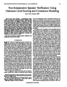
Figure 1: Example Comparison of LTF (F1, F2 and F3 density estimations in bold, means in dotted lines)
case study described in [1] used plots as shown in Figure 1 to compare the LTFs. However, in [1], there was only one comparison made and the authors found a big difference in the formant means. For rejection of speakers, this method might be sufficient if there are big enough differences in the means, but as one might guess from Figure 1, and as Nolan and Grigoras pointed out: There may also be useful information in the shape of the distribution of the estimates for each formant [...].
Grigoras extended this approach to compute likelihood ratios based on the density estimations of formant frequencies on distinct vowel phonemes ([a], [e], [i], [o]) as well as on LTFs [2]. Also, Rose [3] proposed the comparison of vowel phonemes by likelihood ratio computation. In many forensic cases, the expert has to deal with insufficiently described languages, and hence an investigation of vowel phonemes might be difficult. The advantage of the LTF distributions as shown in Figure 1 is that one does not have to distinguish phonemes and is thus timeindependent and text-independent. The remaining question is: how can we compute similarities from LTF distributions?
The d-variate Gaussian function is given by T −1 1 1 f (x; µ, Σ) = p e− 2 (x−µ) Σ (x−µ) , d (2π) det(Σ)
where µ is the mean and Σ is the covariance matrix. d can be any positive integer whose value is determined by the number of features incorporated into every feature vector. A Gaussian mixture density is a weighted sum of M Gaussian distribution functions f (x; µi , Σi ) f (x; µ1 , . . . , µM , Σ1 , . . . , ΣM ) =
One problem is that formant features like F1, F2, F3, as well as the corresponding bandwidths, are usually not independent from each other [3] [4] [5]. If they would be modeled separately in a Bayesian framework, the resulting likelihood ratio scores could not be combined since they would be based on dependent variables. This is of great importance in forensics, where correlated evidence has to be avoided. Hence, our approach models the distribution of multidimensional feature vectors using the well known UBM-GMM framework [6] which has been successfully applied to cepstral feature vectors. Like the approach of Nolan et al. [1] and Grigoras [2], the order of the features is ignored by assuming statistical independence.
(3)
M X
pi f (x; µi , Σi ),
i=1 M X
pi = 1,
(4)
i=1
where pi ≥ 0 are the mixture weights. Therefore a GMM consisting of M Gaussians can be specified by λ := (pi , µi , Σi )i=1,...,M .
(5)
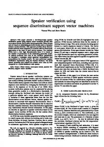
Here, (pi , µi , Σi ) is a tuple consisting of the model parameters, while M is the number of components or mixtures. Every distribution of d-variate feature vectors can thus be described by λ. Full covariance matrices are used to model correlations. This enables us to model the within-speaker variability, see for example Figure 2, where a bivariate GMM based on 8 mixture components is shown. The peaks on the z-axis represent the most frequent F2-F3 configurations, while the shape of the structure reflects the variabilities. For every training recording, a GMM is generated, representing the speakers’ typical formant feature distributions. Additionally, a universal background model (UBM) is created, based on a collection of feature vectors from many different speakers. The UBM represents the reference population. The free statistical software R [7] was used for the model generation, using the mclust [8][9][10][11] package. Similarities of feature vectors X from one speaker and a speaker model λ are expressed by the likelihood, the product of the Gaussian mixture density (see Equation 4). For a set of feature vectors X (see Equation 1) and a speaker model λ (see Equation 5), the likelihood that the feature vectors come from this model is measured via computation of P (X | λ) =
n Y
f (xi | λ),
(6)
i=1
Figure 2: Bivariate GMM for F2 and F3 based on 8 mixture components (density shown on z-axis)
where f (xi | λ) is the Gaussian mixture density function for the specified model λ.
We start by extracting a set of feature vectors for every speaker recording X = {x1 , . . . , xn }, (1)
Every speaker verification test is a comparison of the likelihood of the test feature vectors in the speaker model and the UBM. This is expressed in the likelihood ratio
where every vector
LR =
xi1 xi = ... xid
(2)
is a feature vector of length d. The training feature sets were used for speaker model generation. This was accomplished as follows:
P (X | λspeaker ) . P (X | λUBM )
(7)
The likelihood for λspeaker represents similarity, while λUBM represents typicality. Thus a high likelihood ratio supports the hypothesis that the test feature vectors come from the same speaker while a low likelihood ratio supports the hypothesis that the test feature vectors come from different speakers. For numerical reasons, the log likelihood ratio was computed.
3. Data Base 68 male adult German speakers from the Pool 2010 corpus [12] were used for the experiment. In this corpus, read and spontaneous speech was elicited in a neutral condition, a telephone condition and a Lombard condition. The present study focuses on spontaneous speech in the neutral condition. Spontaneous speech was obtained within a laboratory setting by letting subjects describe a series of pictures in a dialog situation where they had to avoid certain words. In order to make the recordings more realistic forensically, they were played and transmitted through real mobile phone connections. The resulting recordings were edited by hand to eliminate all consonantal information and other speech portions where the formant structure was unclear. Formant tracking by peak picking was applied to this edited material. Any remaining tracking errors were manually corrected and plausibility was checked. These procedures were applied with the Wavesurfer [13] software. The signals were downsampled to 8 kHz. The LPC analysis was set to find 4 formants (only the first three were used due to the telephone filtering, which made F4 unreliable1 ), the analysis window length (Hamming window) was at 0.049 seconds, the LPC order was 12, the preemphasis factor was 0.7, and values were obtained every 10 ms. The method described here corresponds to LTF analysis (long-term distribution of LPC formant estimates) as proposed in [1]. As pointed out in [1], LTF analysis can capture anatomical vocal tract characteristics as well as habitual speaker specifics, such as a palatalized setting and other supralaryngeal voice qualities. A practical advantage of LPC analysis is that it can be applied to languages not spoken by the expert, since no segmentation into phonological units is necessary. The training set was created by using the first half of the formant measurements for every speaker recording, while the test set was generated by using the second half of the formant measurements. Additionally, the test feature vector sets were halved to increase the number of comparisons. The signal duration of the used signal for the training set was about 22 seconds and about 11 seconds for the test set. This can be considered as a plausible scenario in forensic case work regarding bandwidth limiting and signal duration. Henceforth, the formant center frequency features will be abbreviated to F1, F2 and F3, and the corresponding bandwidth features to BW1, BW2 and BW3. 18 speaker measurements were used to create the Universal Background Model (UBM) by pooling all formant features together and estimating one GMM to represent the reference population. The number of mixtures was M = 8 for both UBM and single speaker models. This value was determined experimentally. The speaker features from the remaining 50 speakers were used for the tests. In total, there were 100 × 50 = 5000 tests, 100 same-speaker comparisons and 4900 differentspeaker comparisons. Every comparison resulted in a likelihood ratio score. The equal error rates were computed and a Detection Error Tradeoff plot (DET plot) [15] was created.
4. Results and Discussion To investigate the contribution of the six different features obtained, several feature vectors with different dimensionality and formant features were used and compared. The resulting equal 1 Note,
however, that the measurements of F1 might be affected by the telephone transmission as well [14].
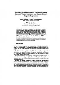
error rates are listed in Table 1, and the corresponding DET plot is shown in Figure 3. Table 1: Equal error rates for different features Features EER F1+F2 0.096 F2+F3 0.105 F1+F2+F3 0.053 F1+F2+BW1+BW2 0.042 F2+F3+BW2+BW3 0.060 F1+F2+F3+BW1+BW2+BW3 0.030
Figure 3: DET plot As can be seen in Table 1 and Figure 3, using two formant features gives the worst performance observed. Using all three formants leads to an improvement. By including the corresponding formant bandwidths, the equal error rate can be reduced additionally. The best performance with an equal error rate of 3 % can be observed using all three formant frequencies and the corresponding bandwidths. The experiment used a relatively small corpus, due to the amount of manual work which had to be done to exclude measurement errors. As a result, the UBM was only based on 18 speakers, which might not adequately represent a reference population. Experiments with larger numbers of speakers will have to be done to investigate the impact of the reference population. The within-speaker variation was included in the models by using full covariance matrices. This approach differs from Grigoras’ [2] and Rose’s [3], who used univariate density estimations, bivariate density estimations, and Gaussian distributions. However, the number of components, as well as the model parameter estimation, might lead to inadequate representations of the feature distributions and hence lead to verification errors. Future experiments should focus on the model generation process, especially since the model parameters can be related directly to the speakers’ vocal tract configurations. These should thus be easier to interpret than, for example, cepstral coefficients which are used in other automatic approaches.
However, we want to highlight the relation of formant features and cepstral features. Since, for example, Mel frequency cepstral coefficients (MFCCs) represent the spectral envelope of the signal with little pitch information, they reflect the vocal tract configurations with its variabilities as well as formant features (see, for example, Darch et al. [16] for the relation between formants and MFCC). While MFCC features were developed and optimized empirically to discriminate within speakers (automatic speech recognition) and between speakers (automatic speaker recognition), formant features are acoustic correlates of vocal tract cavity resonances. Interpretation of evidence in terms of speech samples can be related directly to speakers’ anatomical and physiological characteristics when using formant features, while cepstral coefficients need to be transformed if they should be interpretable in the same way [16]. The all pole model best fits on non-nasalized vowels. However, cepstral coefficients can be interpreted as model vocal tract resonances but do not include a speech production model. By using GMMs we avoided likelihood ratio combinations from different distributions, which is a problem recognized in [2] and [3]. Nevertheless, by looking at the log likelihood ratio value at the EER (i. e. the likelihood ratio values for all six feature vector configurations under investigation that gives the EERs), it could be observed that it ranges from about -100 to -3 (depending on the features used). This might be caused by modeling inadequacies resulting from practical and numerical problems with parameter estimations (e. g. model initialization, number of mixtures). A stable and robust front-end still has to be found. Also, comparison with other automatic speaker verification front-ends will have to be conducted. We have used a realistic data base by choosing telephonetransmitted speech of short duration. However, some performance degrading influences on the formant features may remain (for example differences and mismatches in speaking styles), which have to be carefully addressed in forensic applications.
5. Conclusions We have provided a new method for speaker verification based on formant features. In a semi-automatic procedure, those features were extracted and processed by an automatic UBMGMM verification system. This is an extension of the methods proposed in [1], [2] and [5]. Here, the covariance of formant features is included in the speaker models. In comparison with state-of-the-art automatic speaker verification systems, the proposed method has two important advantages. First, the feature vector space has a small dimensionality (2 to 6). Second, the speaker models can be related directly to the configuration of the vocal tract and hence reflect the vocal tract configuration not only as an average, but also the speaker-specific variations expressed in the entire distribution.
6. Acknowledgments Many thanks to Anja Moos at Saarland University for performing the formant measurements as part of her MA research, as supported by a research grant from the International Association for Forensic Phonetics and Acoustics (IAFPA). The work was supervised by Michael Jessen and Bill Barry.
7. References [1] F. Nolan and C. Grigoras, “A case for formant analysis in forensic speaker identification,” Speech, Language and the Law, vol. 12, no. 2, pp. 143–173, 2005. [2] C. Grigoras, “Forensic Voice Analysis Based on Long Term Formant Distributions,” in 4th European Academy of Forensic Science Conference, June 2006. [3] P. Rose, Forensic Speaker Identification. Taylor & Francis, 2002. [4] P. Rose, “Accounting for correlation in linguistic-acoustic likelihood ratio-based forensic speaker discrimination,” in IEEE Odyssey 2006: The Speaker and Language Recognition Workshop, 2006. [5] P. Rose, “Forensic speaker recognition at the beginning of the twenty-first century - an overview and a demonstration,” Australian Journal of Forensic Sciences, no. 37, pp. 49–72, 2005. [6] D. A. Reynolds, T. F. Quatieri, and R. B. Dunn, “Speaker verification using adapted gaussian mixture models,” Digital Signal Processing, vol. 10, pp. 19–41, 2000. [7] R Development Core Team, R: A Language and Environment for Statistical Computing, R Foundation for Statistical Computing, Vienna, Austria, 2008, ISBN 3900051-07-0. [Online]. Available: http://www.R-project. org [8] J. D. Banfield and A. E. Raftery, “Model-Based Gaussian and Non-Gaussian Clustering,” Biometrics, vol. 49, pp. 803–821, 1993. [9] C. Fraley and A. E. Raftery, “MCLUST: Software for model-based cluster analysis,” Journal of Classification, vol. 16, pp. 297–306, 1999. [10] C. Fraley and A. E. Raftery, “Model-based clustering, discriminant analysis, and density estimation,” Journal of the American Statistical Association, vol. 97, pp. 611–631, 2002. [11] C. Fraley and A. E. Raftery, “MCLUST Version 3 for R: Normal Mixture Modeling and Model-Based Clustering,” University of Washington, Department of Statistics, Tech. Rep. 504, September 2006. [12] M. Jessen, O. K¨oster, and S. Gfroerer, “Influence of vocal effort on average and variability of fundamental frequency,” Speech, Language and the Law, vol. 12, no. 2, pp. 174–213, 2005. [13] http://www.speech.kth.se/wavesurfer/. [14] H. J. K¨unzel, “Beware of the ’telephone effect’: the influence of telephone transmission on the measurement of formant frequencies,” Speech, Language and the Law, vol. 8, no. 1, pp. 80–99, 2001. [15] A. Martin, G. Doddington, T. Kamm, M. Ordowski, and M. Przybocki, “The DET curve in assessment of detection task performance,” in Proc. Eurospeech ’97, 1997, pp. 1895–1898. [16] J. Darch, B. Milner, X. Shao, and Y. Qin, “Predicting formant frequencies from MFCC vectors,” in Proc. of International Conference on Acoustics Speech and Signal Processing (ICASSP 2005), 2005, pp. 941–944.