SPECIAL FUNCTIONS AND PATHWAYS FOR PROBLEMS IN ASTROPHYSICS: AN ESSAY IN HONOR OF A.M. MATHAI Hans J. Haubold 1 , Dilip Kumar 2 , Seema S. Nair 2 , Dhannya P. Joseph
2
Abstract The paper provides a review of A.M. Mathai’s applications of the theory of special functions, particularly generalized hypergeometric functions, to problems in stellar physics and formation of structure in the Universe and to questions related to reaction, diffusion, and reaction-diffusion models. The essay also highlights Mathai’s recent work on entropic, distributional, and differential pathways to basic concepts in statistical mechanics, making use of his earlier research results in information and statistical distribution theory. The results presented in the essay cover a period of time in Mathai’s research from 1982 to 2008 and are all related to the thematic area of the gravitationally stabilized solar fusion reactor and fractional reaction-diffusion, taking into account concepts of non-extensive statistical mechanics. The time period referred to above coincides also with Mathai’s exceptional contributions to the establishment and operation of the Centre for Mathematical Sciences, India, as well as the holding of the United Nations (UN)/European Space Agency (ESA)/National Aeronautics and Space Administration (NASA) of the United States/ Japanese Aerospace Exploration Agency (JAXA) Workshops on basic space science and the International Heliophysical Year 2007, around the world. Professor Mathai’s contributions to the latter, since 1991, are a testimony for his social conscience applied to international scientific activity. c 2010, FCAA – Diogenes Co. (Bulgaria). All rights reserved. °
134
H. Haubold, D. Kumar, S.S. Nair, D.P. Joseph 1. BIOGRAPHICAL NOTES: Professor Dr. A.M. Mathai
Arakaparampil Mathai Mathai was born on 28 April 1935, in Arakulam in the Idukki district of Kerala, India. He is the eldest son of Aley and Arakaparampil Mathai. He completed his High School education in 1953 with record marks in St. Thomas High School, Palai. He then entered St. Thomas College in Palai, obtained his BSc degree in mathematics in 1957 and went to the University of Kerala, Trivandrum, where he completed his MSc degree in statistics in 1959 with first class, first rank, and a golden medal. He joined St. Thomas College as a lecturer from 1959 to 1961. In 1961, he was awarded a Canadian Commonwealth Scholarship and went to the University of Toronto were he completed an MA and a PhD in mathematics and mathematical statistics in only three years, the minimum required time. He then joined McGill University in Montreal - one of the most prestigious universities in North America - where he was Assistant Professor of Mathematics and Statistics, 1964-1968, Associate Professor, 1968-1978, and Full Professor, 1979-2000. Since 2000, he is Emeritus Professor in Mathematics and Statistics at McGill University, Montreal, Canada. He served and is currently serving on editorial boards of a number of journals and he has supervised over 30 Master’s students and 5 PhD students. Currently he is the Director of the Centre for Mathematical Sciences, Trivandrum and Pala Campuses, Kerala, India which he is developing into an national, regional, and international centre of excellence for research in the mathematical sciences. The holding of Seven six-week SERC Schools in 1995, 2000, 2005, 2006, 2007, 2008, and 2009 are a testament of highest achievements in teaching and research in the mathematical sciences for the Centre. A.M. Mathai is a Fellow of the National Academy of Sciences, India, and a Fellow of the Institute of Mathematical Statistics, United States of America. He is an Elected Member of the International Statistical Institute, The Netherlands. He is the Founder of the Canadian Journal of Statistics, Canada, and the Founder of the Statistical Science Association of Canada (now, Statistical Society of Canada). Professor Mathai is a Honorary Member of the International Scientific Organizing Committee of the United Nations/European Space Agency/National Aeronautics and Space Administration of the United States of America/Japanese Aerospace Exploration Agency Workshops on basic space science which have been held, since 1991, in India, Costa Rica, Colombia, Nigeria, Egypt, Sri Lanka, Germany, Honduras, Jordan, France, Mauritius, Argentina, China, United Arab Emirates,
SPECIAL FUNCTIONS AND PATHWAYS . . .
135
India, Japan, Bulgaria, and South Korea. Professor Mathai is author or coauthor of fourteen research level books, seven undergraduate-graduate level books, and more than thirty edited and co-edited proceedings. More than 250 published research papers in journals from around the world are showing the breadth of the array of topics that he has tackled as well as the depth, the complexity and the originality of his published results put him in a class all his own. All these publications concern A.M. Mathai’s research areas with significant research contributions in mathematical statistics, applied statistics, probability, physics, mathematical physics, astrophysics, information theory, mathematics, and specific problems in biological models, orthogonal polynomials, dispersion theory, axiomatization of basic statistical concepts, pollution problems, and transportation problems. An electronic library, recording all of A.M. Mathai’s publications, is under preparation at the United Nations in Vienna. Around the world, A.M. Mathai is known for being very energetic, exceptionally industrious and remarkably gifted. Those individuals who have the good fortune to be close acquaintances of his are also aware of his moral integrity and his social conscience. The latter was particularly beneficial to have him as the advisor in the organization of scientific activities under the umbrella of the United Nations. 2. Astrophysical Thermonuclear Functions Stars are gravitationally stabilized fusion reactors changing their chemical composition while transforming light atomic nuclei into heavy ones. The atomic nuclei are supposed to be in thermal equilibrium with the ambient plasma (Maxwell-Boltzmann). The majority of reactions among nuclei leading to a nuclear transformation are inhibited by the necessity for the charged particles to tunnel through their mutual Coulomb barrier (Gamow). As theoretical knowledge and experimental verification of nuclear cross sections increases it becomes possible to refine analytic representations for nuclear reaction rates. 2.1. The Integrals The standard case of the thermonuclear function contains a nuclear cross section, the energy dependent term of a Taylor series, and the MaxwellBoltzmann distribution function, def
I1 (z, ν) =
Z ∞ 0
y ν e−y e−zy
−1 2
dy,
(1)
136
H. Haubold, D. Kumar, S.S. Nair, D.P. Joseph
where y = E/kT and z = 2π(µ/2kT )1/2 Z1 Z2 e2 /¯ h. Considering dissipative collision processes in the thermonuclear plasma, cut off of the high energy tail of the Maxwell-Boltzmann distribution may occur, thus we write, def
I2 (z, d, ν) =
Z d 0
y ν e−y e−zy
1 −2
dy,
(2)
where d denotes a certain typically high energy threshold. Accommodating screening effects in the standard thermonuclear function we have to use nuclear cross section and the Maxwell-Boltzmann distribution function which leads to Z ∞
def
I3 (z, t, ν) =
0
y ν e−y e−z(y+t)
1 −2
dy,
(3)
where t is the electron screening parameter. Finally, if due to plasma effects a depletion of the Maxwell- Boltzmann distribution has to be taken into account, the thermonuclear function can be written in the following form Z ∞
def
I4 (z, δ, b, ν) =
0
δ
y ν e−y e−by e−zy
−1 2
dy,
(4)
where the parameter δ exhibits the enhancement or reduction of the highenergy tail of the Maxwell-Boltzmann distribution. Mathematical/statistical techniques can be used for deriving closed-form representations of the above thermonuclear functions. 2.2. Closed-form Representation of the Integrals For z > 0 and ν ≥ 0, we have I1 (z, ν) =
Z ∞ 0
Ã
1
ν −y −zy − 2
y e
e
dy = π
− 12
G3,0 0,3
!
¯
z 2 ¯¯ . 4 ¯0, 12 ,1+ν
(5)
For z > 0, d > 0, and ν ≥ 0, we have I2 (z, d, ν) =
Z d 0
y ν e−y e−zy
1 −2
∞ d1+ν X (−d)r 3,0 dy = 1 G1,3 π 2 r=0 r!
Ã
¯
z 2 ¯¯ν+r+2 4d ¯ν+r+1,0, 12
We have I3 (z, t, ν)
def
=
et
ν X
(νr )(−t)ν−r [I1 (z, r) − I2 (z, t, r)] ,
!
. (6) (7)
r=0
and I4 (z, δ, b, ν)
ref
=
P∞ (−b)r r=0
r!
I1 (z, ν + rδ).
(8)
SPECIAL FUNCTIONS AND PATHWAYS . . .
137
We obtain I1 (z, ν) ∼ 2
³ 2 ´1/3 µ ¶ 1 Ã 2 ! 2ν+1 6 −3 z4 π 2 z
3
e
4 Ã
I2 (z, d, ν) ∼ dν+1 e−d
z2 4d
µ ¶1
Ã
π I3 (z, t, ν) ∼ 2 3 I4 (z, δ, b, ν) ∼ 2
2
et
³
!−1/2
z2 4
e
−2
³
!1 6
e
−3
z2 4d
z2 4
,
(9)
´1/2
,
(10)
´1/3 Ã
z2 4
ν
!1
3
− t ,
³ 2 ´1/3 ³ 2 ´δ/3 µ ¶ 1 Ã 2 ! 2ν+1 6 −3 z4 −b z4 π 2 z
3
4
e
e
,
(11)
(12)
all as z → ∞. 2.3. Extension of the Thermonuclear Functions Using Pathway Model Further, the four integrals can be extended by using the pathway model of Mathai which covers the Tsallis statistics. Then we get the general integrals given below. The extended integral in the standard case of the thermonuclear function which contains a non-resonant cross-section and with a pathway distribution function is Z ∞
def
I1α (z, ν) =
0
1
y ν [1 + (α − 1)y]− α−1 e−zy
−1 2
dy, α > 1,
(13)
where y = E/kT and z = 2π(µ/2kT )1/2 Z1 Z2 e2 /¯ h. If we consider cut-off of the high energy tail of the Maxwell-Boltzmann distribution, then the extended non-resonant thermonuclear function is def
I2α (z, d, ν) =
Z d 0
1
y ν [1 − (1 − α)y] 1−α e−zy
−1 2
dy,
(14)
1 where d = 1−α . The extended integrals I3α and I4α can be obtained by using I1α and I2α using some arithmetics.
2.4. Closed form evaluation of the extended integrals For z > 0, ν ≤ 0 and α > 1, we have 1
I1α (z, ν) =
π− 2
(α −
³ ´ G3,1 1,3 1 ν+1 1) Γ α−1
Ã
¯
1
!
(α − 1)z 2 ¯¯2− α−1 +ν . ¯ 1 4 0, 2 ,1+ν
(15)
138
H. Haubold, D. Kumar, S.S. Nair, D.P. Joseph
For z > 0, ν ≤ 0, d =
1 1−α
and α < 1, we have
I2α (z, d, ν) =
dν+1 Γ(d + 1) 1
π2
G3,0 1,3
Ã
¯
z 2 ¯¯ν+d+2 4d ¯ν+1,0, 12
!
.
(16)
It is to be noted that as α → 1, by using the Stirling approximation I1α and I2α will become I1 . 2.5. Further Reading Anderson, W.J., Haubold, H.J., and Mathai, A.M.: 1992, Astrophysical thermonuclear functions, Astrophysics and Space Science, 214, 49-70. Bergstrom, Iguri, S., and Rubinstein, H.: 1999, Constraints on the variation of the fine structure constant from big bang nucleosynthesis, Physical Review D60, 045005. Critchfield, C.L.: 1972, Analytic forms of the thermonuclear function. In: Cosmology, Fusion, and Other Matters. George Gamow Memorial Volume, E dited by F. Reines, University of Colorado Press, Colorado, 186-191. Davis Jr., R.: 1996, A review of measurements of the solar neutrino flux and their variation, Nuclear Physics, Proceedings Supplement, B48, 284-298. Fowler, W.A.: 1984, Experimental and theoretical nuclear astrophysics: The quest for the origin of the elements, Reviews of Modern Physics 56, 149-179. Haubold, H.J. and Kumar, D.: 2008, Extension of thermonuclear functions through the pathway model including Maxwell-Boltzmann and Tsallis distributions, Astroparticle Physics, 29, 70-76. Mathai, A.M., Haubold, H.J.: 1988, Modern Problems in Nuclear and Neutrino Astrophysics, Akademie-Verlag, Berlin. Mathai, A.M., Haubold, H.J.: 2002, Review of mathematical techniques applicable in astrophysical reaction rate theory, Astrophysics and Space Science, 282, 265-280. Mathai, A.M., Haubold, H.J.: 2008, Special Functions for Applied Scientists, Springer-Verlag, New York. Mathai, A.M., Saxena, R.K.: 1973, Generalized Hypergeometric Functions with Applications in Statistics and Physical Sciences, Lecture Notes in Mathematics Vol. 348, Springer-Verlag, Berlin. Saxena, R. K.: 1960, Proceedings of the National Academy of Sciences, India 26, 400-413.
SPECIAL FUNCTIONS AND PATHWAYS . . .
139
3. Solar Structure in Terms of the Gauss Hypergeometric Function Hydrostatic equilibrium and energy conservation determine the conditions in the gravitationally stabilized solar fusion reactor. We assume a matter density distribution varying non-linearly through the central region of the Sun. The analytic solutions of the differential equations of mass conservation, hydrostatic equilibrium, and energy conservation, together with the equation of state of the perfect gas and a nuclear energy generation rate ² = ²0 ρn T m , are given in terms of Gauss’ hypergeometric function. This model for the structure of the Sun gives the run of density, mass, pressure, temperature, and nuclear energy generation through the central region of the Sun. Because of the assumption of a matter density distribution, the conditions of hydrostatic equilibrium and energy conservation are separated from the mode of energy transport in the Sun. 3.1. Hydrostatic Equilibrium In the following we are concerned with the hydrostatic equilibrium of the purely gaseous spherical central region of the Sun generating energy by nuclear reactions at a certain rate. For this gaseous sphere we assume that the matter density varies non-linearly from the center outward, depending on two parameters δ and γ, ρ(x) = ρc fD (x), (17) fD (x) = [1 − xδ ]γ ,
(18)
where x denotes the dimensionless distance variable, x = r/R¯ , 0 ≤ x ≤ 1, R¯ is the solar radius, δ > 0, γ > 0 and γ is kept a positive integer in the following considerations. The choice of the density distribution reveals immediately that ρ(x = 0) = ρc is the central density of the configuration and ρ(x = 1) = 0 is a boundary condition for hydrostatic equilibrium of the gaseous configuration. For the range 0 ≤ x ≤ 0.3 the density distribution can be fit numerically to computed data for solar models by choosing δ = 1.28 and γ = 10. The choice of restricting x to x ≤ 0.3 is justified by looking at a Standard Solar Model which shows that x ≤ 0.3 comprises what is considered to be the gravitationally stabilized solar fusion reactor. More precisely, 95% of the solar luminosity is produced within the region x < 0.2(M < 0.3M¯ ). The half-peak value for the matter density occurs at x = 0.1 and the half-peak value for the temperature occurs at x = 0.25. The region x ≤ 0.3 is also the place where the solar neutrino fluxes are generated.
140
H. Haubold, D. Kumar, S.S. Nair, D.P. Joseph
As we are concerned with a spherically symmetrical distribution of matter, the mass M (x) within the radius x having the density distribution is M (x) = M¯ fM (x), (19) ( 3δ + 1)( 3δ + 2) · · · ( 3δ + γ) 3 3 3 x 2 F1 (−γ, ; + 1; xδ ), (20) γ! δ δ where M¯ denotes the solar mass and 2 F1 (.) is Gauss’ hypergeometric function. This equation is satisfying the boundary condition M (x = 0) = 0 and determine the central value ρc of the matter density through the boundary condition M (x = 1) = M¯ , where ρc depends then only on δ and γ of the chosen density distribution. For hydrostatic equilibrium of the gaseous configuration the internal pressure needs to balance the gravitational attraction. The pressure distribution follows by integration of the respective differential equation for hydrostatic equilibrium, making use of the above density distribution and mass distribution, that is 9 M¯2 G 4 fP (x), P (x) = (21) 4π R¯ fM (x) =
"
( 3 + 1)( 3δ + 2) . . . ( 3δ + γ) fP (x) = δ γ! "
#2
γ 1 X (−γ)m 3 2 δ m=0 m!( δ + m)( 2δ + m)
#
γ! 2 2 × 2 − xδm+2 2 F1 (−γ, + m; + m + 1; xδ ) , δ δ ( δ + m + 1)γ
(22)
where G is Newton’s constant and 2 F1 (.) denotes again Gauss’ hypergeometric function. The Pochhammer symbol 2 2 2 ( + m + 1)γ = Γ( + m + 1 + γ)/Γ( + m + 1) δ δ δ often appears in series expansions for hypergeometric functions. This equation gives the value of the pressure Pc at the centre of the gaseous configuration and satisfies the condition P (x = 1) = 0. 3.2. Equation of State We noted that P (x) denotes the total pressure of the gaseous configuration, that is the sum of the gas pressure and the radiation pressure (according to Stefan-Boltzmann’s law). However, the radiation pressure, although the ratio of radiation pressure to gas pressure increases towards the center of the Sun, remains negligibly small in comparison to the gas pressure. Thus,
SPECIAL FUNCTIONS AND PATHWAYS . . .
141
P (x) can be considered to represent the run of the gas pressure through the configuration under consideration. Further, the matter density is so low that at the temperatures involved the material follows the equation of state of the perfect gas. Therefore, the temperature distribution throughout the gaseous configuration is given by µ M¯ fT (x), (23) T (x) = 3 G kNA R¯ "
fT (x) =
#
γ X ( 3δ + 1)( 3δ + 2) · · · ( 3δ + γ) 1 1 (−γ)m γ! δ 2 [1 − xδ ]γ m=0 m!( 3δ + m)( 2δ + m)
"
#
2 γ! 2 − xδm+2 2 F1 (−γ, + m; + m + 1; xδ ) , (24) × 2 δ δ ( δ + m + 1)γ where k is the Boltzmann constant, NA Avogadro’s number, µ the mean molecular weight, and 2 F1 (.) Gauss’ hypergeometric function. The equations for T (x) reveal the central temperature for T (x = 0) = Tc and satisfy the boundary condition T (x = 1) = 0. Since the gas in the central region of the Sun can be treated as completely ionized, the mean molecular weight µ is given by µ = (2X + 43 Y + 21 Z)−1 , where X, Y, Z are relative abundances by mass of hydrogen, helium, and heavy elements, respectively, and X + Y + Z = 1. 3.3. Nuclear Energy Generation Rate Hydrostatic equilibrium and energy conservation are determining the physical conditions in the central part of the Sun. In the preceeding sections, the run of density, mass, pressure, and temperature have been given for a gaseous configuration in hydrostatic equilibrium based on the equation of state of the perfect gas. In the following, a representation for the nuclear energy generation rate, ²(ρ, T ) = ²0 ρn T m , (25) will be sought which takes into account the above given distributions of density and temperature and which can be used to integrate the differential equation of energy conservation throughout the gaseous configuration. In the above equation, n denotes the density exponent, m the temperature exponent, and ²0 a positive constant determined by the specific reactions for the generation of nuclear energy. 3.4. Total Nuclear Energy Generation The total net rate of nuclear energy generation is equal to the luminosity of the Sun, that means the generation of energy by nuclear reactions in
142
H. Haubold, D. Kumar, S.S. Nair, D.P. Joseph
the central part of the Sun has to continually replenish that energy radiated away at the surface. If L(x) denotes the outflow of energy across the spherical surface at distance x from the center, then in equilibrium the average energy production at distance x is Z 3 L(x) = 4πR¯
x
0
dt t2 ρ(t)²(t),
(26)
where ρ(x) and ²(x) are given above. 3.5. Further Reading Chandrasekhar, S.: 1939/1957, An Introduction to the Study of Stellar Structure, Dover Publications Inc., New York. Clayton, D.D.: 1986, Solar structure without computers, American Journal of Physics, 54, 354-362. Haubold, H.J., Mathai, A.M.: 1995, Solar structure in terms of Gauss’ hypergeometric function, Astrophysics and Space Science, 228, 77-86. Haubold, H.J.: 1995, An analytic solar model: Physical principles and mathematical structures, International Journal of Mathematical and Statistical Sciences, 4, 31-41. Haubold, H.J., Mathai, A.M.: 2001, Sun, In: Encyclopedia of Planetary Sciences, Eds. J.H. Shirley and R.W. Fairbridge, Chapman and Hall, New York, 786-794. Mathai, A.M. and Haubold, H.J.: 2008, Special Functions for Applied Scientists, Springer, New York. Mathai, A.M., Saxena, R.K., and Haubold, H.J.: 2009, The H-Function: Theory and Applications, Springer, New York. Stein, R.F.: 1966, in R.F. Stein and A.G.W. Cameron (eds.), Stellar Evolution, Plenum Press, New York. 4. The Fractional Kinetic Equation The subject of this remark is to derive the solution of the fractional kinetic equations. The results are obtained in a compact form containing the Mittag-Leffler function, which naturally occurs whenever one is dealing with fractional integral equations. 4.1. Kinetic Equation and Mittag-Leffler Function In terms of Pochammer’s symbol
SPECIAL FUNCTIONS AND PATHWAYS . . .
143
n
1, n=0 α(α+1)...(α+n−1), n∈N, α6=0
(α)n =
we can express the binomial series as −α
(1 − x)
=
∞ X (α)r xr r=0
r!
, |x| < 1.
The Mittag-Leffler function is defined by ∞ X zn , 0, Eα (x) := Γ(αn + 1) n=0
(27)
(28)
where |a|1/α , Re(β) > 0, which can be established by means of the Laplace integral Z ∞
0
e−pt tρ−1 dt = Γ(ρ)/pρ ,
(33)
where Re(p) > 0, Re(ρ) > 0. The Riemann-Liouville operator of fractional integration is defined as Z t 1 −ν f (u)(t − u)ν−1 du, ν > 0, (34) a Dt f (t) = Γ(ν) a with a Dt0 f (t) = f (t). By integrating the standard kinetic equation
144
H. Haubold, D. Kumar, S.S. Nair, D.P. Joseph
d Ni (t) = −ci Ni (t), (ci > 0), dt
(35)
it is derived that Ni (t) − N0 = −ci
−1 0 Dt Ni (t),
(36)
where 0 Dt−1 is the standard Riemann integral operator. The number density of species i, Ni = Ni (t), is a function of time and Ni (t = 0) = N0 is the number density of species i at time t = 0. By dropping the index i, the solution of its generalized form N (t) − N0 = −cν is obtained as N (t) = N0
−ν 0 Dt N (t),
∞ X (−1)k (ct)νk k=0
Γ(νk + 1)
,
(37) (38)
By virtue of the original definition of the Mittag-Leffler function, we can rewrite this solution in terms of the Mittag-Leffler function in a compact form as N (t) = N0 Eν (−cν tν ), ν > 0. (39) 4.2. Conclusions Solutions are given in terms of the ordinary Mittag-Leffler function and their generalization, which can also be represented as Fox’s H-functions. The classical and the generalized Mittag-Leffler functions interpolate between a purely exponential law and power-like behavior of phenomena governed by ordinary kinetic equations and their fractional counterparts. 4.3. Further Reading Grafiychuk, V., Datsko, B., and Meleshko, V.: 2006, Mathematical modeling of pattern formation in sub- and superdiffusive reaction-diffusion systems, arXiv:nlin.AO/0611005 v3. Haubold, H.J. and Mathai, A.M.: 2000, The fractional kinetic equation and thermonuclear functions, Astrophysics and Space Science, 327, 53-63. Mathai, A.M. and Haubold, H.J.: 2008, Special Functions for Applied Scientists, Springer, New York. Mathai, A.M., Saxena, R.K., and Haubold, H.J.: 2009, The H-Function: Theory and Applications, Springer, New York.
SPECIAL FUNCTIONS AND PATHWAYS . . .
145
Oldham, K.B. and Spanier, J.: 1974, The Fractional Calculus: Theory and Applications of Differentiation and Integration to Arbitrary Order, Academic Press, New York. Saxena, R.K., Mathai, A.M., Haubold, H.J.: 2002, On fractional kinetic equations, Astrophysics and Space Science, 282, 281-287. Saxena, R.K., Mathai, A.M., Haubold, H.J.: 2004, Unified fractional kinetic equation and a fractional diffusion equation, Astrophysics and Space Science, 290, 299-310. Saxena, R.K., Mathai, A.M., and Haubold, H.J.: 2006, Fractional reactiondiffusion equations, Astrophysics and Space Science, 305, 289-296. Srivastava, H.M. and Saxena, R.K.: 2001, Operators of fractional integration and their applications, Applied Mathematics and Computation, 118, 1-52. Tsallis, C.: 2004, What should a statistical mechanics satisfy to reflect nature?, Physica D, 193, 3-34. Turing, A.M.: 1952, The chemical basis of morphogenesis, Philosophical Transactions of the Royal Society of London, B237, 37-72. 5. Generalized Measure of Entropy, the Mathai Pathways, and the Tsallis Statistics When deriving or fitting models for data from physical experiments very often the practice is to take a member from a parametric family of distributions. But it is often found that the model requires a distribution with a more specific tail than the ones available from the parametric family, or a situation of right tail cut-off. The model reveals that the underlying distribution is in between two parametric families of distributions. In order to create a distributional pathway for proceeding from one functional form to another a pathway parameter is introduced and a pathway model is created. This model enables one to go from a generalized type-1 beta model to a generalized type-2 beta model to a generalized gamma model when the variable is restricted to be positive. More families are available when the variable is allowed to vary over the real line. Corresponding multitudes of families are available when the variable is in the complex domain. Originally, Mathai deals mainly with rectangular matrix-variate distributions in the real case and the scalar case is the topic of discussion in the current remark because the scalar case is connected to many problems in physics. Similarly, through
146
H. Haubold, D. Kumar, S.S. Nair, D.P. Joseph
a generalized measure of entropy, an entropic pathway can be devised that leads to different families of entropic functionals that produce families of distributions by applying the maximum entropy principle.
5.1. The Pathway Model in the Real Scalar Case For the real scalar case the pathway model for positive random variables is the following: β
f (x) = c xγ−1 [1 − a(1 − α)xδ ] 1−α , x > 0,
(40)
a > 0, δ > 0, β ≥ 0, 1 − a(1 − α)xδ > 0, γ > 0 where c is the normalizing constant and α is the pathway parameter. The normalizing constant in this case is the following: ³
γ
c =
δ[a(1 − α)] δ Γ Γ
¡γ ¢ δ
³
Γ γ
=
δ[a(α − 1)] δ Γ Γ
¡γ ¢ δ
³
Γ
β α−1
γ δ
+
β 1−α
³
γ δ
´
´
+1
+1
β α−1
−
β 1−α
, for α < 1
(41)
´
´ , for
γ 1 − > 0, α > 1 α−1 δ
(42)
γ
=
δ (aβ) δ ¡ ¢ , for α → 1. Γ γδ
(43)
As α < 1, f (x) is the generalized type-1 beta model. When α > 1, f (x) is the generalized type-2 beta model and f (x) is the generalized gamma model as α → 1. For various values of the pathway parameter α a path is created so that one can see the movement of f (x) towards a generalized gamma density. From Fig. 1(a) we can see that, as α moves away from 1 the function f (x) moves away from the origin and it becomes thicker tails and less peaked. From Fig. 1(b) we can see that when α moves from −∞ to 1, the curve becomes thicker tails and less peaked. From the path created by α we note that we obtain densities with thicker or thinner tail compared to generalized gamma density.
SPECIAL FUNCTIONS AND PATHWAYS . . .
147
(a)
(b) Fig 1, (a): Behaviour of f (x) for various values of α > 1, γ = 2, δ = 2 and β = 1. (b): Behaviour of f (x) for various values of α < 1, γ = 2, δ = 2 and β = 1.
148
H. Haubold, D. Kumar, S.S. Nair, D.P. Joseph 5.2. Pathway Model from a Generalized Entropy Measure
A generalized entropy measure of order α is a generalization of Shannon entropy and it is a variant of the generalized entropy of order α. In the discrete case the measure is the following: Consider a multinomial population P = (p1 , . . . , pk ), pi ≥ 0, i = 1, . . . , k, p1 + . . . + pk = 1. Define the function Pk
2−α i=1 pi
Mk,α (P ) =
−1
α−1
lim Mk,α (P ) = −
α→1
, α 6= 1, −∞ < α < 2
k X
pi ln pi = Sk (P )
(44) (45)
i=1
by using l’Hopital’s rule. In this notation 0 ln 0 is taken as zero when any pi = 0. Thus it is a generalization of Shannon entropy Sk (P ). Note that it is a variant of Havrda-Charv´at entropy Hk,α (P ) and Tsallis entropy Tk,α (P ), where Pk pαi − 1 , α 6= 1, α > 0 (46) Hk,α (P ) = i=1 21−α − 1 and Pk pα − 1 Tk,α (P ) = 1=1 i , α 6= 1, α > 0. (47) 1−α We will introduce another measure associated with the above and parallel to R´enyi entropy Rk,α in the following form: ∗ Mk,α (P ) =
ln
³P
2−α k i=1 pi
´
, α 6= 1, −∞ < α < 2. α−1 The R´enyi entropy is given by ³ ´ Pk α p ln i=1 i Rk,α (P ) = , α 6= 1, α > 0. 1−α
(48)
(49)
5.2.1. Continuous Analogue The continuous analogue to the generalized entropy measure is the following: R∞
Mα (f ) =
2−α dx −∞ [f (x)]
−1
(50) α−1 1−α f (x)dx − 1 E[f (x)]1−α − 1 −∞ [f (x)] = , α 6= 1, α < 2, α−1 α−1
R∞
=
where E[·] denotes the expected value of [·]. Note that when α = 1, E[f (x)]1−α = E[f (x)]0 = 1.
SPECIAL FUNCTIONS AND PATHWAYS . . .
149
It is easy to see that the generalized entropy measure is connected to Kerridge’s “inaccuracy” measure. The generalized inaccuracy measure is E[q(x)]1−α where the experimenter has assigned q(x) for the true density f (x), where q(x) could be an estimate of f (x) or q(x) could be coming from observations. Through disturbance or distortion if the experimenter assigns [f (x)]1−α for [q(x)]1−α then the inaccuracy measure is Mα (f ). 5.2.2. Distributions with Maximum Generalized Entropy Among all densities, which one will give a maximum value for Mα (f )? Consider all possible functions f (x) such that f (x) ≥ 0 for all x, f (x) = 0 outside (a, b), Ra < b, f (a) is the same for all such f (x), f (b) is the same for all such f , ab f (x)dx < ∞. Let f (x) be a continuous function of x with R continuous derivatives in (a, b). Let us maximize ab [f (x)]2−α dx for fixed α and over all functional f , under the conditions that the following two moment-like expressions be fixed quantities: Z b a
(γ−1)(1−α)
x
f (x)dx = given, and
Z b a
x(γ−1)(1−α)+δ f (x)dx = given (51)
for fixed γ > 0 and δ > 0. Consider U = [f (x)]2−α − λ1 x(γ−1)(1−α) f (x) + λ2 x(γ−1)(1−α)+δ f (x), α < 2, α 6= 1, (52) where λ1 and λ2 are Lagrangian multipliers. Then the Euler equation is the following: ∂U = 0 ⇒ (2 − α)[f (x)]1−α − λ1 x(γ−1)(1−α) + λ2 x(γ−1)(1−α)+δ = 0 ∂f λ2 λ1 x(γ−1)(1−α) [1 − xδ ] (53) ⇒ [f (x)]1−α = (2 − α) λ1 1
⇒ f (x) = c xγ−1 [1 − η(1 − α)xδ ] 1−α , (54) δ where λ1 /λ2 is written as η(1 − α) with η > 0 such that 1 − η(1 − α)x > 0 since f (x) is assumed to be non-negative. By using the conditions above we can determine c and η. When the range of x for which f (x) is nonzero is (0, ∞) and when c is a normalizing constant, then f (x) is the pathway model of Mathai in the scalar case where α is the pathway parameter. When γ = 1, δ = 1 in f (x), then f (x) produces the power law. The form above for various values of λ1 and λ2 can produce all the four forms: 1
1
α1 xγ−1 [1 − β1 (1 − α)xδ ]− 1−α , α2 xγ−1 [1 − β2 (1 − α)xδ ] 1−α for α < 1 and
150
H. Haubold, D. Kumar, S.S. Nair, D.P. Joseph
1
1
α3 xγ−1 [1 + β3 (α − 1)xδ ]− α−1 , α4 xγ−1 [1 + β4 (α − 1)xδ ] α−1 for α > 1 with αi , βi > 0, i = 1, 2, 3, 4. But out of these, the second and the third forms can produce densities in (0, ∞). The first and fourth will not be converging. 5.3. Extended Riemann-Liouville Fractional Integral Through Pathway Model A new fractional integral operator associated with the pathway model of A.M. Mathai, generalizes the classical Riemann-Liouville fractional integration operator. Also, this newly introduced integral operator reduces to the Laplace integral transform, when the pathway parameter α → 1. The integral operator called pathway fractional operator is obtained as an extension of left-sided Riemann-Liouville fractional integral operator, and is defined as follows: Let f (x) ∈ L(a, b), η ∈ C, 0, a > 0 and the ”pathway parameter ” α < 1, then Z [ x ] η a(1−α) a(1 − α)t (1−α) (η,α) ] [1 − f (t)dt, (55) (P0+ f )(x) = xη x 0 where f (t) is an arbitrary function. η aη ] 1−α → e− x t . Then, the operator gets the When α → 1− , [1 − a(1−α)t x form Z ∞ aη aη (η,1) e− x t f (t) dt = xη Lf ( ), (56) P0+ = xη x 0 i.e. reduces to the Laplace transform of f with parameter aη x . When α = 0, a = 1, then replacing η by η − 1 the integral becomes a left-sided Riemann-Liouville fractional integral. If we substitute f (t) by t 2 F1 (η + β, − γ; η; 1 − x )f (t), then we have the form of the Saigo operator. Naturally, by associating f (t) with other elementary or special functions, (55) takes a form of Mathai’s “pathway model” extensions of other (leftsided) operators of generalized fractional calculus, as the Erd´elyi-Kober, Kiryakova operators, etc. 5.6. Further Reading Gell-Mann, M. and Tsallis, C. (Eds.): 2004, Nonextensive Entropy: Interdisciplinary Applications. Oxford University Press, New York. Joseph, D. P.: 2009, Gamma distribution and extensions by using pathway idea, Statistical Papers, Accepted, DOI 10.1007/s00362-009-0231-y.
SPECIAL FUNCTIONS AND PATHWAYS . . .
151
Kiryakova, V.S.: 1986, On operators of fractional integration involving Meijers G-function, Comp. Rend. Acad. Bulg. Sci., 39, No 10, 25-28. Kiryakova, V.: 1994, Generalized Fractional Calculus and Applications. Longman Sci. & Techn. and J. Wiley & Sons, Harlow - N. York. Kiryakova, V.: 2006, On two Saigo’s fractional integral operators in the class of univalent functions. Fract. Calc. Appl. Anal., 9, No 2, 159-176. Mathai, A.M. and Haubold, H.J.: 2008, Special Functions for Applied Scientists, Springer, New York. Mathai, A.M., Saxena, R.K., and Haubold, H.J.: 2009, The H-Function: Theory and Applications, Springer, New York. Mathai, A.M.: 2005, A pathway to matrix-variate gamma and normal densities, Linear Algebra and Its Applications, 396, 317-328. Mathai, A.M. and Haubold, H.J.: 2007, Pathway model, superstatistics, Tsallis statistics, and a generalized measure of entropy, Physica A, 375, 110-122. Mathai, A.M. and Haubold, H.J.: 2008, Pathway parameter and thermonuclear functions, Physica A, 387, 2462-2470. Mathai, A.M. and Haubold, H.J.: 2008, On generalized distributions and pathways, Physics Letters A, 372, 2109-2113. Mathai, A.M. and Rathie, P.N.: 1975, Basic Concepts in Information Theory and Statistics: Axiomatic Foundations and Applications, Wiley Halsted, New York and Wiley Eastern, New Delhi. Nair, Seema. S.: 2009, Pathway fractional integration operator. Fract. Calc. Appl. Anal., 12, No 4, 237-252. Nicolis, G. and Prigogine, I.: 1977, Self-organization in Non-equilibrium Systems: From Dissipative Structures to Order Through Fluctuations, John Wiley and Sons, New York. Tsallis, C.: 2009, Introduction to Nonextensive Statistical Mechanics - Approaching a Complex World, Springer, New York. 6. Gravitational Instability in a Multicomponent Cosmological Medium The paper presents results for deriving closed-form analytic solutions of the non-relativistic linear perturbation equations, which govern the evolution of inhomogeneities in a homogeneous spatially flat multicomponent cosmological model. Mathematical methods to derive computable forms of the perturbations are outlined.
152
H. Haubold, D. Kumar, S.S. Nair, D.P. Joseph 6.1. Introduction
These closed-form solutions are valid for irregularities on scales smaller than the horizon. They may be used for analytical interpolation between known expressions for short and long wavelength perturbations. We present the physical parameters relevant to the problem and the fundamental differential equations for arbitrary polytropic index γi and a radiation or matter dominated Universe, respectively. Solutions of this fundamental equation are provided for relevant parameter sets including the polytropic index γi and the expansion law index η. To catalogue these solutions in closed-form, the theory of Meijer’s G-function will be employed. 6.2. Some Parameters of Physical Significance The growth of density inhomogeneities can begin as soon as the Universe is matter-dominated. Baryonic inhomogeneities cannot begin to grow until after decoupling because until then, baryons are tightly coupled to the photons. After decoupling, when the Universe is matter-dominated and baryons are free of the pressure support provided by photons, density inhomogeneities in the baryons and any other matter components can grow. Actually the time of matter-radiation equality is the initial epoch for structure formation. In order to fill in the details of structure formation one needs ”initial data” for that epoch. The initial data required include, among others, (1) the total amount of non-relativistic matter in the Universe, quantified by Ω0 , and (2) the composition of the Universe, as quantified by the fraction of critical density, Ωi = ρi /ρc , contributed by various components of primordial density perturbations (i= baryons, Wimps, relativistic particles, etc.). Here the critical density ρc is the total matter density of the Einstein-de Sitter Universe. Speculations about the earliest history of the Universe have provided hints as to the appropriate initial data: Ω0 = 1 from inflation; 0.015 ≤ ΩB ≤ 0.15 and ΩW IM P ∼ 0.9 from inflation, primordial nucleosynthesis, and dynamical arguments. In the following we P assume that Ωi = 1, Ωi = const. The cosmological medium is considered to be unbounded and that there may be a uniform background of relativistic matter. It is further assumed that the matter is only slightly perturbed from the background cosmological model. This assumption may give a good description of the behavior of matter on large scales even when there may be strongly nonlinear clustering on small scales (primordial objects). Also assumed is that matter can be approximated as an ideal fluid with pressure a function of density alone. It consists of i components having the densities ρi and velocities of sound βi2 = dPi /dρi ∝ ργi −1 , when an equation of state
SPECIAL FUNCTIONS AND PATHWAYS . . .
153
Pi ∝ ργi
(57)
has been taken into account. The i components of the medium are interP related through Newton‘s field equation ∆φ = 4πG ρi , containing the P combined density ρi of all components. Superimposed upon an initially homogeneous and stationary mass distribution shall be a small perturbation, represented by a sum of plane waves δρi δ= = δi (t)eikx , (58) ρ where k = 2πa/λ defines the wave number k and λ is the proper wavelength. In the linear approach the system of second order differential equations describing the evolution of the perturbation in the non-relativistic component i is m X d2 δi a˙ dδi 2 2 + k βi δi = 4πG ρj δj , i = 1, ..., m, (59) + 2( ) dt2 a dt j=1 where for all perturbations the same wave number k is used. This equation is valid for all sub-horizon-sized perturbations in any non-relativistic species, so long as the usual Friedmann equation for the expansion rate is used. Although the following investigation of closed-form solutions of the fundamental differential equation governing the evolution of inhomogeneities in a multicomponent cosmological medium is quite general, it will be presented within the context of the inflationary scenario. Therefore in the following we consider an Einstein-de Sitter Universe with zero cosmological constant. After inflation the Friedmann equation for the cosmological evolution reduces to 8πG a˙ ( )2 = H 2 = ρ. (60) a 3 The continuity equation gives ρ ∝ a−3 and one has a ∝ t2/3 and ρi = Ωi /(6πGt2 ). During the expansion the Hubble parameter changes as H = ηt−1 , where the expansion law index is η = 21 in the radiation-dominated epoch and η = 23 in the matter-dominated epoch respectively. The wave number is proportional to a−1 so that k 2 βi2 = ki2 t2(1−η−γi ) , where now the constants ki come from both the wave vector and the velocity of sound. If ki = 0 the sound velocity βi equals zero, in which case the adiabatic index γi loses its sense. Defining the parameter αi = 2(2 − η − γi ) that absorbs the adiabatic index as well as the type of expansion law, we can write: t2 δ¨i (t) + 2ηtδ˙i (t) + ki2 tαi δi =
m 2X Ωj δj (t), 3 j=1
i = 1, . . . , m,
(61)
154
H. Haubold, D. Kumar, S.S. Nair, D.P. Joseph
and dots denote derivatives with respect to time. We introduce a time operator ∆ = td/dt and change the dependent variable, the density perturbation δi (t), dealing with the function Φi instead of δi by setting δi (t) = tα Φi (t). The equation for the function Φi is then given by m 2X ∆2 Φi + bi Φi = Ωj Φj , 3 j=1 where
µ
Φi = t−α δi , bi = ki2 tαi − α2 , αi = 2(2 − η − γi ), α = −
2η − 1 . 2
(62)
Observing that ΣΩj = 1 and operating on both sides of the differential equation for the Φi by ∆2 , we obtain the fundamental equation m 2 2X ∆4 Φi + ∆2 (bi Φi ) − (∆2 Φi + bi Φi ) = − bj Ωj Φj , i = 1, . . . m. (63) 3 3 j=1
As indicated above for η, the values 32 and 12 are significant and in what follows it will be assumed that 2 ≥ γi ≥ 32 . We have chosen the range of values of γi for physical as well as mathematical reasons as will be evident later in the analysis. For some of these parameter values we will consider a multicomponent medium. Consider the special case b1 = k12 tα1 −
(2η − 1)2 , 4
(2η − 1)2 (64) 4 of the fundamental equation. Let k = 0. For this case the parameters are the following: b2 = b3 = · · · = bm = b = k 2 tα −
(
b∗1 , b∗2
=±
(2η − 1)2 4α12
)1 2
(
a∗1 , a∗2
= −1 ±
(
, b∗3 , b∗4 "
=±
"
1 (2η − 1)2 2 + 4 3 α12
1 (2η − 1)2 2 2 + − Ω1 4 3 3 α12
#) 1 2
,
#) 1 2
.
(65)
6.3. Solution when the Parameters Differ by Integers The general solution are for finite values of t and for the cases that the do not differ by integers. At two points, namely (η = 23 , γi = 53 ) and (η = 32 , γi = 1) one has b∗1 − b∗3 = −1 and b∗4 − b∗2 = −1.
b∗j ’s
SPECIAL FUNCTIONS AND PATHWAYS . . .
155
6.4. Modifications of the G0j s for the Cases (η = 32 , γi = 1) and (η = 23 , γi = 35 ) Consider, for x = k12 tα1 /α12 , α1 6= 0, ³
a∗ +1,a∗ +1
1,2 G1 = G2,4 x |b∗1,b∗ ,b∗2,b∗
=
1 2πi
1
Z
2
Γ( 14
L
3
´
4
+ s)Γ(−a∗1 − s)Γ(−a∗2 − s)x−s ds . Γ( 54 − s)Γ(− 14 − s)Γ( 49 − s)
(66)
Note that a zero coming from Γ(− 14 − s) at s = − 14 coincides with a pole coming from Γ( 14 + s) at s = − 14 . This can be removed by rewriting as follows: Z Γ( 54 + s)Γ(−a∗1 − s)Γ(−a∗2 − s)x−s ds 1 G1 = − . (67) 2πi L Γ( 54 − s)Γ( 34 − s)Γ( 49 − s) Evaluating this expression as the sum of the residues at the poles of Γ( 54 +s) one has Γ(−a∗1 + 54 )Γ(−a∗2 + 45 ) 14 Γ( 10 4 )Γ(2)Γ( 4 ) 5 10 14 5 × 2 F3 (−a∗1 + , −a∗2 + ; , 2, ; −x). 4 4 4 4 Evaluating G4 , also in the same way, one has the following: 5
G1 = −x 4
³
a∗ +1,a∗ +1
1,2 G4 = G2,4 x |b∗1,b∗ ,b∗2,b∗
Z
= = =
4
1
2
(68)
´
3
Γ(− 54 + s)Γ(−a∗1 − s)Γ(−a∗2 − s) −s 1 x ds 2πi L Γ( 34 − s)Γ( 54 − s)Γ(− 14 − s) Z Γ(− 14 + s)Γ(−a∗1 − s)Γ(−a∗2 − s) −s 1 x ds − 2πi L Γ( 34 − s)Γ( 94 − s)Γ(− 14 − s) 1 1 ∗ ∗ 1 Γ(− 4 − a1 )Γ(− 4 − a2 ) −x− 4 Γ( 12 )Γ(2)Γ(− 12 ) 1 1 1 1 × 2 F3 (− − a∗1 , − − a∗2 ; , 2, − ; −x). 4 4 2 2
(69)
Thus the complete solution in this case is of the form Φ1 = c1 G1 + c2 G2 + c3 G3 + c4 G4 , where c1 , c2 , c3 , c4 are arbitrary constants.
(70)
156
H. Haubold, D. Kumar, S.S. Nair, D.P. Joseph 6.5. Conclusion
We have presented closed-form solutions of the non-relativistic linear perturbation equations which govern the evolution of inhomogeneities in a spatially flat multicomponent cosmological medium. The general solutions are catalogued according to the polytropic index γi and the expansion law index η of the multicomponent medium. All general solutions are expressed in terms of Meijer’s G-function and their Mellin-Barnes integral representation. The proper use of this function simplifies the derivation of solutions of the linear perturbation equations and opens ways for its numerical computation. 6.6. Further Reading Gailis, R.M. and Frankel, N.E.: 2006, Two-component cosmological fluids with gravitational instabilities, Journal of Mathematical Physics, 47, 062505. Gailis, R.M. and Frankel, N.E.: 2006, Short wavelength analysis of the evolution of perturbations in a two-component cosmological fluid, Journal of Mathematical Physics, 47 062506. Gottloeber, S., Haubold, H.J., Muecket, J.P., and Mueller, V.: 1988, Early Evolution of the Universe and Formation of Structure, Akademie-Verlag, Berlin. Haubold, H.J. and Mathai, A.M.: 1994, Computational aspects of the gravitational instability problem for a multicomponent cosmological medium, Astrophysics and Space Science, 214, 139-149. Haubold, H.J. and Mathai, A.M.: 1998, Structure of the Universe, In: Encyclopedia of Applied Physics, Ed. G.L. Trigg, Vol. 25, Wiley-VCH Verlag GmbH, Weinheim - New York, 47-81. Mathai, A.M.: 1989, On a system of differential equations connected with the gravitational instability in a multicomponent medium in Newtonian cosmology, Studies in Applied Mathematics, 80,75-93. Mathai, A.M., Saxena, R.K.: 1973, Generalized Hypergeometric Functions with Applications in Statistics and Physical Sciences. Lecture Notes in Mathematics, Vol. 348, Springer-Verlag, Berlin. Mathai, A.M. and Haubold, H.J.: 2008, Special Functions for Applied Scientists, Springer, New York. Mathai, A.M., Saxena, R.K., and Haubold, H.J.: 2009, The H-Function: Theory and Applications, Springer, New York.
SPECIAL FUNCTIONS AND PATHWAYS . . .
157
Mather, J.C. et al.: 1992, Early results from the Cosmic Background Explorer (COBE), AIP Conference Proceedings, Vol. 245, American Institute of Physics, New York, 266-276. Peebles, P.J.E.: 1980, The Large-Scale Structure of the Universe, Princeton University Press, Princeton. 7. Developing Basic Space Science World-Wide Since 1991, Professor Dr. A.M. Mathai was a member of the International Scientific Organizing Committee of all UN/ESA/NASA/JAXA workshops and provided his expertise in the mathematical and statistical sciences to the development of the scientific programmes of these workshops. From 1991 to 2004 the workshops focused on basic space science. From 2005 to 2009 the workshops were dedicated to the International Heliophysical Year 2007. Beginning in 2010, the workshops will develop the International Space Weather Initiative. 7.1. Further Reading Wamsteker, W., Albrecht, R., and Haubold, H.J. (Eds.): 2004, Developing Space Science World-Wide: A Decade of UN/ESA Workshops, Kluwer Academic Publishers, Dordrecht Boston London. Thompson, B.J., Gopalswamy, N., Davila, J.M., and Haubold, H.J. (Eds.): 2009, Putting the ”I” in IHY: The United Nations Report for the International Heliophysical Year 2007, Springer, New York. Briand, C., Antonucci, E., Gopalswamy, N., Eichhorn, G., Sakurai, T., Mathai, A.M., and Haubold, H.J. (Eds.): 2009, International Heliophysical Year 2007, Second European General Assembly, Italy, and Third UN/ESA/ NASA Workshop, Japan. Earth, Moon, and Planets, Vol. 104, 1-360. 1
Office for Outer Space Affairs, United Nations Vienna International Centre P.O. Box 500, A-1400 Vienna, AUSTRIA Received: August 26, 2009 e-mail:
[email protected] 2
Centre for Mathematical Sciences – Pala Campus Arunapuram P.O., Pala, Kerala – 686574, INDIA e-mails:
[email protected] ,
[email protected] ,
[email protected]