A New Hybrid Direct/Specialized Approach for Generating Inverse Neural Models FERNANDO MORGADO DIAS1, ANA ANTUNES1, 2ALEXANDRE MANUEL MOTA 1 Escola Superior de Tecnologia de Setúbal do Instituto Politécnico de Setúbal Campus do IPS, Estefanilha, 2914-508 Setúbal 2 Departamento de Electrónica e Telecomunicações Universidade de Aveiro, 3810 Aveiro PORTUGAL 1 {fmdias,aantunes}@est.ips.pt
[email protected] Abstract: - In the literature the most common proposed solutions for training inverse neural models are the direct (or general) and specialized methods. The second one being considered as more reliable to produce correct inverse models has nevertheless some drawbacks in the implementation. The present paper introduces a hybrid solution that copes with the problems and limitations of both solutions. The hybrid solution merges the training and evaluation stages for producing an inverse model, ensuring the production of a correct inverse which is goal directed and does not need iterative algorithms to be produced. This new solution was developed within the preparation of an automated procedure for creating models for control purposes, which consists in a combination of Genetic Algorithms and Neural Networks. Key-Words: - Feedforward Neural Networks, Direct Inverse Control, Internal Model Control, Measurement Noise, Genetic Algorithm, Inverse Modelling, Early Stopping, Direct Training and Specialized Training
1 Introduction The issue of producing Artificial Neural Network (ANN) models of systems to be used for modeling or control purposes has deserved a reasonable slice of interest in the ANN community. Most of the new proposed solutions concern the use of new types of ANN or the development of new algorithms, while the structures used are, in almost every application in spite of the extensive description of the many solutions for the training structures present in [16], the classical direct (or general) and the specialized training methods as reported in [1]. Nevertheless, it is known that the direct training method has severe disadvantages and the specialized training method is difficult to implement for most of the algorithms. The present work reports a rather simple hybrid solution to cope with the disadvantages of both architectures. This solution resulted from the development of an automated procedure for creating models for control purposes, which consists in a combination of Genetic Algorithms and Neural Networks. The hybrid solution can be used also in nonautomated construction of models.
2 Direct, Specialized and COEM Training Methods The simplest approach is the direct method, which is closely related to forward modeling. A block diagram of this type of training can be seen in figure 1. However simple, this approach has some drawbacks[1]: • The learning procedure is not goal directed. The training signal must be chosen to sample over a wide range of system inputs and the actual operational inputs may be hard to define a priori. The actual goal in the context is to make the system output behave in a desired way and thus the training signal in direct inverse modeling does not correspond to the explicit goal. • In situations where the mapping is not 1:1 an incorrect inverse can be obtained. To avoid these problems, another way of training inverse models is present in the literature (for example in [1] and [2]): specialized inverse model training. The models and plant are connected according to figure 2.
u(k)
Plant
y(k)
+
uhat(k) -
Inverse Model
eu(k)
Fig. 1. Structure for inverse model according to the direct training method.
training,
eu(k)
Figure 3 represents Indirect Inverse Adaptation (IIA)[16]. In this structure an inverse model is used instead of a direct model. The inverse model allows estimating uhat from the output of the plant enabling the calculation of the error eu, which will be used to adapt the controller and the inverse model. In the case of the Controller Output Error Method (COEM) the inverse model and the controller are the same. The only change this fact produces is that calculations have to be performed in two steps using the same model.
Direct Model
r(k)
Inverse Model
uhat(k)
Plant
y(k)
-
ey(k)
r(k)
u(k)
Controller
+
+
eu(k)
Fig. 2. Structure for inverse model training, according to the specialized training method. The inverse model is connected in series with the plant, but since usually the internal states of the Plant are unknown and do not allow performing the necessary calculations to report the error ey (between plant output and desired output) to the output of the inverse model eu, a direct model is placed in parallel with plant. Through this model it is possible to obtain the error eu from the error ey using the appropriate derivative calculations. This structure is supposed to overcome the problems mentioned for the direct training because the network is trained in a situation similar to the one that the NN will assume in a control situation. Nevertheless the specialized training method has some drawbacks: • Although it has been shown to work properly even when the forward model is not exact (as referred in [1]), this method is difficult to use with noisy systems. • The structure requires, in principle, an iterative version of the training algorithm. This limits the training to the algorithms for which there are iterative versions. The second problem makes it impossible to use for instance the Levenberg-Marquardt algorithm, for which a true iterative version has not yet been developed and the use of iterative versions like the ones proposed for the Gauss-Newton methods are clearly not as effective as the Levenberg-Marquardt algorithm.
Plant
y(k)
eu(k)
-
uhat(k)
Inverse Model
Fig. 3. Structure for Indirect Inverse Adaptation. The COEM solution or the IIA solution, present the same type of advantages and problems that have been reported for the specialized training solution.
3 The Hybrid Approach Usually the evaluation of the quality of a model is done using a second sequence of data called the test sequence. Some authors also use a third sequence, which is used for comparing different neural models [3]. The hybrid approach is a mixture of the structure and quality evaluation and consists of the following steps: 1. Produce a direct model. 2. Train the inverse model using a direct structure. 3. Evaluate the quality of the inverse model using a simulation of Direct Inverse Control (DIC) as depicted in figure 4, where the plant is replaced by its model. This solution, although very simple and intuitive, does in fact improve the development of inverse models. Analysing the problems of both architectures it is possible to verify that they are solved: • The hybrid approach is goal directed since the models are now evaluated in a simulation of control, which is exactly the
• •
r(k)
situation where the inverse model will be used. There is no risk of obtaining an incorrect inverse since the inverse will be evaluated in control simulation. This solution does not need iterative versions of the algorithms and therefore does not impose limitations on the algorithm to be used. Inverse Model
u(k)
Plant
4.1
The Automated Procedure
The combination of GAs and ANN developed falls in the second situation pointed above: learning neural network topologies. In the present implementation that means optimising the architecture of a fully connected FNN of one hidden layer, with linear output, hyperbolic tangents as hidden layer’s activation function and AutoRegressive with eXogenous input (ARX) architectures.
y(k)
Fig. 4. Structure for Direct Inverse Control. The signal r(k) is the reference, u(k) the control signal and y(k) the output signal. Although the hybrid approach can be used in a general way, it was developed during the implementation of a combination of Genetic Algorithms and Feedforward Neural Networks (FNN) for the choice of the best architecture. This combination will be described shortly in the next sections, in order to present the results obtained with the hybrid approach.
4 Combination of Genetic Algorithms and Artificial Neural Networks Genetic Algorithms and Neural Networks are both inspired by computation in biological systems. A good deal of biological neural architecture is determined genetically. It is therefore not surprising that as some neural network researchers explored how neural systems are organized that the idea of evolving neural networks should arise [4]. This sort of combination has already originated enough work to enable the production of many surveys and reviews around this research field from which [4][5][6][7] are only a small sample. As pointed out in [4] the three major ways that have been receiving attention from researchers developing combinations between GAs and ANNs are: • Setting weights in fixed architectures. • Learning neural network topologies. • Select training data and interpret the output behavior of ANN. More recently other trends have appeared as Genetic Encoding strategies [8] is an example.
4.1.1 Structure of the Networks The structure of the network is composed of four parameters: number of past inputs, number of past outputs, number of neurons in the hidden layer and number of training iterations. The first two parameters allow choosing the past information to be used, using only the information that is important. The number of neurons in the hidden layer allows the adjustment of the network size to the complexity of the system to be modelled. Using the number of training iterations also as a parameter gives the possibility to use early stopping. The parameters and their ranges are summarized in table 1. The choice of the ranges involves previous work done with the system used as test bench [9][10]. The networks are represented in a simple bit string, which will be used by a GA algorithm to choose the best network. The evaluation of each model contained in the bit stings is based on the Mean Square Error (MSE) between the model and the sequence used for testing, when the direct model is used or the error between the reference signal and the output when the inverse model is used. TABLE I - PARAMETERS TO USE IN THE OPTIMIZATION PROCEDURE. Parameter Number of bits Range of values Past outputs 2 1:4 Past inputs 2 1:4 Hidden 4 1:16 neurons Iterations 8 1:256 In the latter situation the hybrid direct/specialized approach for generating inverse neural models is used, because the initial tests that were done using a simple test sequence showed that although the evaluation of the models reported good quality, they were not good enough to control the real system.
Each model proposed holds a value for each of the parameters, forming a different network. The models are trained using the Levenberg-Marquardt (LM) algorithm because of its fastest convergence. During the identification and control tasks the NNSYSID [3] and NNCTRL [4] toolboxes for MATLAB were used. 4.1.2 Evolution of the Networks As stated, the evolution of the networks is done using a GA algoritm. The GA optimisation is especially useful when there is no deterministic solution for the problem or the range of solutions is too wide for an exhaustive search and local minimum can be acceptable. Both situations are true in the ANN field, which makes GAs particularly fit for this evolution. The algorithm implemented includes Crossover, Mutation and Elitism according to what is detailed below. Using a small population of 20 individuals, a strong elitism of 20% is assumed, crossover of one site splicing is performed and all the individuals are subjected to mutation except the elites.The mutation operator is a binary mask generated randomly according to a selected rate that is superposed to the existing binary codification of the population changing some of the bits. Crossover is performed over 50% of the population, always including the elites. The individuals are randomly selected with equal opportunity to create the new population. The fitness of the solution is the Mean Square Error obtained between the output of the model and the desired output. The desired output can be the output values in the training set for the direct model or the reference used in the DIC simulation for the inverse model. The fittest solution is the one with the lower fitness value. A global perspective of the optimization solution can be obtained from figure 5. Generation of Initial Population - This block represents the generation of the initial population, which consists basically of generating a random population. Network Parameter Extraction – The bit string is sliced according to the size of the parameters, which are converted using their ranges. Training of each Individual – Each element of the population, after the extraction of the parameters, represents a ANN that is trained with the Levenberg-Marquardt algorithm according to the training structures defined for the direct and inverse models. Evaluation of each Individual – Each individual’s fitness is now evaluated using a test sequence or
direct inverse control according to the type of model. Selection of the elite – After the evaluation phase, the individuals are now sorted according to their fitness and the best 20% will constitute the elite. Generation of Initial Population
Network Parameter Extraction
R e p r o d u c t i o n
Training of each Individual (Levenberg-Marquardt Algorithm)
Evaluation of each Individual
Selection of the Elite
No Finished?
Yes
Stop
Fig. 5. Representation of the optimisation solution. The block diagram shows the operations performed in each generation of the genetic algorithm. The overall results are evaluated to check if the search is over. The search might terminate by reaching a certain number of iterations or by achieving a certain quality of the models. If these
conditions are met the search is terminated otherwise the reproduction process is activated. Reproduction - The new population is generated by reproduction using mutation and crossover.
5 The Plant The plant used is a reduced scale prototype kiln and the tests reported concern the implementation of the temperature control loop. Figure 6 shows a scheme of the modules composing the system. An electrical resistor driven by a power controller heats the kiln and the temperature is measured by a B type thermocouple. The sensor and the actuator are connected to a Hewlett Packard HP34970A Data Logger that supplies real-time data to MATLAB using the RS232C serial line. The Data Logger though a helpful tool limits the measurement to temperatures superior to 300ºC and the thermocouple introduces measurement noise, which makes identification more complex. This approach allows the use of the entire MATLAB powerful environment together with real-time capability.
Fig. 7. Picture of the kiln and electronics.
6 Control Structures The control structures used to test the optimization procedure are: Direct Inverse Control and Internal Model Control. These structures are briefly presented in the following subsections.
6.1 Heating Element
Power Module
thermocouple
Data Logger
Direct Inverse Control (DIC)
Direct inverse control is the simplest solution for control that consists of connecting in series the inverse model and the plant as can be seen in figure 4. If the inverse model is accurate the output of the system y(k) will follow the reference r(k). PC
Fig. 6. Schematic of the modules composing the system. The kiln is completely closed and operates around 750ºC having as superior limit of operation 1000ºC. The Data Logger is used as the interface between PC and the rest of the system. Since the Data Logger can be programmed using a protocol called Standard Commands for Programmable Instruments (SCPI), a set of functions have been developed to provide MATLAB with the capability to communicate through the RS232C port to the Data Logger. A picture of the system can be seen in figure 7. The kiln can be seen in the center and at the lower half the prototypes of the electronic modules and the cooling fans.
6.2
Internal Model Control (IMC)
Internal Model Control is a structure that allows the error feedback to reflect the effect of disturbance and plant mismodelling. In fact it can be shown [9] that a good match between forward and inverse models is enough to have good control and that with this structure disturbance’s influence is also reduced. The basic IMC structure can be seen in figure 8.
6.3 Adapting the Control Structures to use Neural Network Models The structure presented in the subsection A can be used with Neural Network (NN) models without the need of major changes, but the structure used in section B needs some refinements to work properly [11].
r(k) +
-
Inverse Model
u(k)
Input sequence (training and test set, respectively)
y(k)
Plant
1
+ 0.5
Direct Model
-
0
0
1000
2000
yhat(k)
3000
4000
5000
4000
5000
Output sequence 800
e(k)
700 600
Fig. 8. Structure for Internal Model Control. The signal r(k) is the reference, u(k) the control signal, y(k) the output signal, yhat(k) the estimate of the output and e(k) the error between the output and the estimate. The good match between forward and inverse models, referred above translates to having the forward model outputs feedback to the input of the inverse and direct model instead of the outputs of the plant. This means that the inverse model will implement the following equation: r ( k + 1), yhat ( k ),..., yhat ( k − n y + 1) u( k ) = g u( k − t d ),..., u( k − nu − t d + 1)
(1)
instead of:
r (k + 1), y (k ),..., y (k − n y + 1) u (k ) = g u (k − t d ),..., u (k − n u − t d + 1)
(2)
Where ny is the number of previous output samples used, nu is number of previous control signal samples used and td is the time delay of the system. During the identification and control tasks the NNSYSID [12] and NNCTRL [13] toolboxes for MATLAB were used.
500 400 300
0
1000
2000
3000 time (samples)
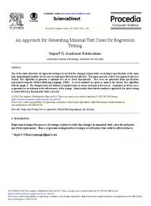
Fig. 9. Training and test signals. TABLE II - PARAMETERS OF THE BEST MODELS OBTAINED. Model\ NU NY Nhidden Iteration NGen Parameters Previous 2 2 4 50 n.a. Direct New Direct 3 3 7 58 49 Previous 2 2 5 70 n.a. Inverse New Inverse 1 1 3 225 89 The models denoted as previous are the models used in previous work [9] [10] and are inserted here as a reference for comparison. These models were optimised using the author’s knowledge about the system and neural models. Figures 10 and 11 show the evolution of the error in the direct and inverse models through the generations. -5
4.6
Evolution of the best solution
x 10
4.5
4.4
7 The Models Obtained Figure 9 shows the training and test signals used for training the models, separated by the hashed vertical line. Table 2 shows the details of the best solution obtained for direct and inverse models, where NU stands for number of past inputs, NY is the number of past inputs, Nhidden is the number of hidden neurons in the hidden layer, Iteration is the number iterations during which the network was trained and NGen is the number of generation used for the NN evolution.
Test Error
4.3
4.2
4.1
4
3.9
3.8
0
10
20
30
40
50 Generations
60
70
80
90
100
Fig. 10. Evolution of the best solution found for the direct model through the generations. Although this type of combination between Gas and NN is considered to be very slow, in the present case the evolution is very fast when compared with the
typical applications. This is due to the fact that the ranges are carefully selected in the beginning and to the efficiency of the LM training algorithm.
Internal Model Control - Kiln Temperature and Set Point 800 600 400 200
Evolution of the best solution
0
20
40
60
80
0
20
40
60
80
0
20
40
60
80
100 Error
120
140
160
180
200
100 120 Control Signal
140
160
180
200
140
160
180
200
5
0.035
0
0.03
-5
0.025
Test Error
1.5 0.02
1 0.5
0.015
0 0.01
0.005
0
0
10
20
30
40 50 Generations
60
70
80
90
8 The Real Time Control Action The new models from table 2 were used to implement DIC and IMC according to section V. The results obtained can be seen in figures 12 and 13 and they confirm the expectation that this technique can produce models of good quality. Direct Inverse Control - Kiln Temperature and Set Point 800 600 400
0
20
40
60
80
0
20
40
60
80
0
20
40
60
80
100 Error
120
140
160
180
200
100 120 Control Signal
140
160
180
200
140
160
180
200
5
0
-5 1.5 1 0.5 0
120
Fig. 13. Internal Model Control results.
Fig. 11. Evolution of the best solution found for the inverse model through the generations.
200
100 time x30s
100 time x30s
120
Fig. 12. Direct Inverse Control results. Table 3 presents a summary of the results in terms of Mean Square Error (MSE) and a comparison between the best results obtained for both control strategies in present and previous work. As can be seen the results obtained show an enormous improvement in the results when compared with the results obtained previously.
TABLE III - SUMMARY OF THE RESULTS OBTAINED FOR BOTH CONTROL STRATEGIES. MODELS\ DIC (MSE) IMC STRATEGY (MSE) Previous Models 5.14 0.96 Models 2 0.58 0.30
9 Conclusion A new hybrid technique has been presented for replacing the classical structures for inverse modelling (direct and specialized). This technique is called hybrid since it is composed of training and evaluation. The training is done according to the direct training structure and the test is done by simulation of control. The hybrid approach overcames the problems usually pointed out for both the classical solutions. The technique has been tested using an automated procedure, which consists of a combination of GAs and ANN and the results of a test using a real system under measurement noise condition show that this technique can produce models with very good quality. The hybrid technique was used with an optimisation algorithm, based in Genetic Algorithms to search for the best models, The evolution performed is short in terms of generations but is quite consuming in CPU time. References: [1] K. J. Hunt, D. Sbarbaro, R. Zbikowski and P. J. Gawthrop, ”Neural Networks for Control Systems-A Survey”, Automatica, vol.28, nº6, pp1083-1112, 1992
[2] M. Nørgaard, “System Identification and Control with Neural Networks”. PhD Thesis, Department of Automation, Technical University of Denmark, 1996. [3] Hagan, Demuth e Beale, “Neural Network Design”, PWS Publishing Company, 1996. [4] D. Whitley, “Genetic Algorithms and Neural Networks”, Genetic Algorithms in Engineering and Computer Science, edited by J. Periaux and G. Winter, published by John Wiley and Sons, 1995. [5] J. Schaffer, D. Whitley and L. Eshelman, “Combination of Genetic Algorithms and Neural Networks: The state of the art”, Combination of Genetic Algorithms and Neural Networks, IEEE Computer Society, 1992. [6] X. Yao, “Evolutionary artificial neural networks”, International Journal of Neural Systems, 4, 203-222, 1993. [7] T. Hussain, “Methods of Combining Neural Networks and Genetic Algorithms”, Tutorial Presentation, ITRC/TRIO Researcher Retreat, Kingston, Ontario, Canada,1997. [8] P. Köhn, “Genetic Encoding Strategies for Neural Networks”, Information Processing and Management of Uncertainty in Knowledgebased Systems, Granada, Spain, 1996. [9] F. M. Dias and A. M. Mota, “A Comparison between a PID and Internal Model Control using Neural Networks”, 5th World Multi-Conference on Systemics, Cybernetics and Informatics, Orlando, EUA, 2001. [10] F. M. Dias and A. M. Mota, ”Comparison between different Control Strategies using Neural Networks”, 9th Mediterranean Conference on Control and Automation, Dubrovnik, Croatia, 2001. [11] G. Lightbody and G. W. Irwin, “Nonlinear Control Structures Based on Embedded Neural System Models”, IEEE transactions on Neural Networks, vol.8, no.3, 1997. [12] M. Nørgaard, “Neural Network System Identification Toolbox for MATLAB”, Technical Report,1996. [13] M. Nørgaard, Neural Network Control Toolbox for MATLAB, Technical Report,1996. [14] K. J. Hunt and D. Sbarbaro, ”Neural Networks for Nonlinear Internal Model Control”, IEE Proceedings-D, vol.138, no.5, pp.431438, 1991. [15] O. Sørensen, “Neural Networks in Control Applications”, PhD Thesis, Department of Control Engineering, Institute of Electronic Systems, Aalborg University, Denmark, 1994.
[16] H. Andersen, ”The Controller Output Method”, PhD Thesis, Department of Computer Science and Electrical Engineering, University of Queensland, St. Lucia 4072, Australia, 1998.